Article

Spatial Domain-Based Nonlinear Residual Feature Extraction for Identification of Image Operations

1
Faculty of Information Technology, Macau University of Science and Technology, Macau 853, China
2
Zhuhai MUST Science & Technology Research Institute, Zhuhai 519000, China
*
Author to whom correspondence should be addressed.
Appl. Sci. 2020, 10(16), 5582; https://doi.org/10.3390/app10165582
Submission received: 7 July 2020 / Revised: 6 August 2020 / Accepted: 10 August 2020 / Published: 12 August 2020
(This article belongs to the Special Issue Advanced Intelligent Imaging Technology Ⅱ)

Abstract

:
In this paper, a novel approach that uses a deep learning technique is proposed to detect and identify a variety of image operations. First, we propose the spatial domain-based nonlinear residual (SDNR) feature extraction method by constructing residual values from locally supported filters in the spatial domain. By applying minimum and maximum operators, diversity and nonlinearity are introduced; moreover, this construction brings nonsymmetry to the distribution of SDNR samples. Then, we propose applying a deep learning technique to the extracted SDNR features to detect and classify a variety of image operations. Many experiments have been conducted to verify the performance of the proposed approach, and the results indicate that the proposed method performs well in detecting and identifying the various common image postprocessing operations. Furthermore, comparisons between the proposed approach and the existing methods show the superiority of the proposed approach.

1. Introduction

Currently, forgeries of digital images are widely propagated, and it is expected that tampered images will be used more and more in society, including in social media and even scientific discovery. This will cause a serious impact on political and social stability. At the same time, while postprocessing techniques and operations for use with digital images are developing rapidly, the imperceptible modification of digital images is becoming easier. Therefore, ever-increasing attention is being paid to digital image forensics, including detection of forgery and postprocessing operations.
To date, many approaches regarding image forensics have been proposed, such as tracking the history of JPEG compression [1,2,3,4]; revealing the image operations, including contrast enhancement [5,6], resampling [7,8,9,10], and median filtering [11,12,13,14]; detecting the image splicing operations [15,16], revealing frequency domain filtering [17]; and identifying image forgery [18,19]. However, most of these state-of-the-art studies have simply considered specific operations. On the other hand, some of the approaches only perform binary classification. In [1,2,3,4], the authors proposed methods of detecting history of JPEG compression and revealing artifacts caused by image coding. The methods were based on blocks. In [6], Stamm and Liu proposed detecting the occurrence of digital image modification according to contrast enhancement operations in a blind way. In [7], Popescu and Farid proposed detecting the resampling traces and interpolations based on a derivative operator and the radon transformation. In [20], Rao and Ni proposed detecting forgeries in digital images using a deep learning method. In [21], two-class 3D-convolutional neural network (3D-CNN) classifiers were employed for video copy detection. However, in most cases, the features show low feasibility and reasonability, especially when the processing types of the detected images are unknown. For example, if we fed a median-filtered image into a classifier to detect the histogram equalization, it could be classified as a histogram-equalized image or an original image. Either result would be wrong because the feature employed in this approach is specially designed for detecting histogram equalization. Similarly, the accuracy of identifying other image operations will drop significantly if we apply the same classifier. Therefore, an effective forensics approach that can identify various image operations simultaneously is essential and of great importance.
Recently, in [22], a method based on a spatial rich model (SRM) feature was proposed. The SRM was proposed to be used as a steganalysis feature by Fridrich et al. [23]. Multiple nonlinear and linear filters were employed to generate residuals, and then the high-order features were extracted and merged into the SRM features. Experiments were conducted to select the multiple sets of filters, and they can be used under different models to extract the residual information from the image. In [22], Li et al. proposed reducing the dimensionality of the SRM features. Afterward, they applied an ensemble classifier [24] for classification of the various common image postprocessing operations. Experimental results showed that this scheme performed better than most of the related state-of-the-art works; however, there was an obvious downtrend when the size of the observed images was decreased. Furthermore, features in this work were manually designed, and thus they might not be effective enough for identifying the various image operations because of the high complexity. The ensemble classifier [24] is a multiclassifier ensemble method that utilizes the complementary relationships of the classifiers to improve the generalization ability effectively, and it can be used to work with high-dimensional features with significantly lower training complexity. However, to choose the final classifier, most base classifiers are abandoned, and the chosen classifier is the classifier that has the minimum testing error; moreover, the classification ability of a single classifier is weak, and this could affect the detection ability of the final classifier. In our previous work [25], we employed the SRM and deep learning technology for image processing detection and identification, and the results indicated the great potential of applying deep learning technology.
Currently, as a hot research field in machine learning, the deep learning technique has been widely used in multimedia security applications. In this paper, we propose applying the deep learning framework to the field of image forensics for the detection and classification of various operations. As part of the development of deep learning technology, the backpropagation neural network (BPNN) [26] classification method is a nonparametric classification method that is based on traditional statistical theory. It does not need to assume or estimate the probability distribution function of the target. Considering its good adaptability and complex mapping ability, this method can obtain good classification accuracy in pattern classification. However, considering the problem of the BPNN being fully connected in every layer, which leads to difficulty in training, the BPNN has been gradually replaced by the CNN [27]. The CNN proposes the concept of weight sharing, which increases the learning efficiency by greatly reducing the number of free parameters being learned. Thus far, a couple of neural network models have been proposed. LeNet-5 is a classic CNN that defines the classic neural network structure. AlexNet [28] extends the structure of LeNet-5, and it has made great progress in the field of image classification. However, AlexNet uses two layers of 4096 neurons to connect to each other, which makes the network easy to overfit and difficult to train.
To avoid the abovementioned shortcomings and to effectively identify a variety of image operations, in this paper we propose a novel approach by extending our previous work [25]. In our previous work [25], we proposed this framework to identify the various image operations, and the experimental results showed a very good potential of the proposed framework in this application. In that work, the submodel of the spatial rich model (SRM) [23], sub_SRM, was applied for feature extraction. On that basis, in this work, we propose the spatial domain-based nonlinear residual (SDNR) feature extraction method by constructing residual values from locally supported filters in the spatial domain. By applying minimum and maximum operators, diversity and nonlinearity are introduced; moreover, this construction brings nonsymmetry to the distribution of SDNR samples. Then, similarly, we apply a deep learning method of a five-layer CNN to the extracted SDNR features to produce the detection and identification results. Many experiments are conducted to evaluate the performance of the improved approach, and the results show that the improved work can identify more image postprocessing operations when compared with the previous work [25]; this previous work allowed seven operation types to be identified, while this improved method allowed more than twice this number to be identified. Furthermore, the results of using BPNN and AlexNet are tested to show the superiority of the proposed method. The remainder of this paper is arranged as follows: Section 2 presents the proposed approach for identification of image operations, Section 2.1 explains the principle of the proposed SDNR method, and Section 2.2 introduces the employed CNN classifier in detail. Then, Section 3 demonstrates the experiments and discussions. Finally, Section 4 concludes this paper.

2. Proposed Approach for Identification of Image Operations

The design of the feature set plays an important part in classification problems. Fortunately, we can borrow some powerful features from other research fields, such as image classification, computer vision, and image steganalysis. An example is the modern universal steganalytic features, such as SRM [23], which consists of statistics derived from a number of image residuals. In such features, different high-pass filters are used to suppress the image content in different ways, and thus the obtained features can represent different local properties. In this paper, we propose the SDNR by constructing residual values from locally supported filters in the spatial domain. Then, to make use of the extracted SDNR features, we propose applying a deep learning method of a five-layer CNN to the extracted SDNR feature to produce the detection and classification results. The framework of the proposed approach is shown in Figure 1. In Figure 1, it can be seen that there are two major steps: feature extraction with the proposed SDNR method, and feature learning with a five-layer CNN model. In the proposed approach, firstly, we apply the variety of postprocessing operations, including spatial enhancement, spatial filtering, frequency filtering, and lossy compression, to the original images. In this way, the original images are trained and the corresponding postprocessed images are thus produced. Then, the SDNR is employed to the generated images to extract the feature sets. Next, we employ a five-layer CNN model to extract the CNN features from the extracted SDNR feature sets. A patch-sized sliding window is used to scan the extracted SDNR feature sets, and feature fusion is adopted to aggregate the CNN features and thus to obtain the discriminated feature from the image. Afterward, the softmax classifier of the CNN is trained for the detection and identification of the various operations.

2.1. Spatial Domain-Based Nonlinear Residual (SDNR) Feature

The SDNR is constructed from locally supported linear filters in the spatial domain. By applying minimum and maximum operators, the diversity and nonlinearity are thus introduced. In this way, the construction brings nonsymmetry to the distribution of SDNR samples. In Equation (1), the calculation of residual value is expressed, where I and f are the host image and filter, respectively. The corresponding residual of the pixel is calculated by multiplying and summing the corresponding pixel and its adjacent pixels by the filter coefficients. Considering the fact that for edge pixels of the image, the pixel value might not be adequately changed in accordance with the filter coefficients, mirror symmetric filling operations are conducted on the images before applying the filtering operations. That means the images are filled adjacently by border pixel values. After this operation, the size of the residual map does not change.
R i , j = I f = a = M M b = N N f ( a , b ) I ( i a , j b )
where R denotes the residual map, which is calculated from the host image I and the filter f ; denotes the convolution process; and A and B indicate the size of the host image. M = A / 2 and N = B / 2 .
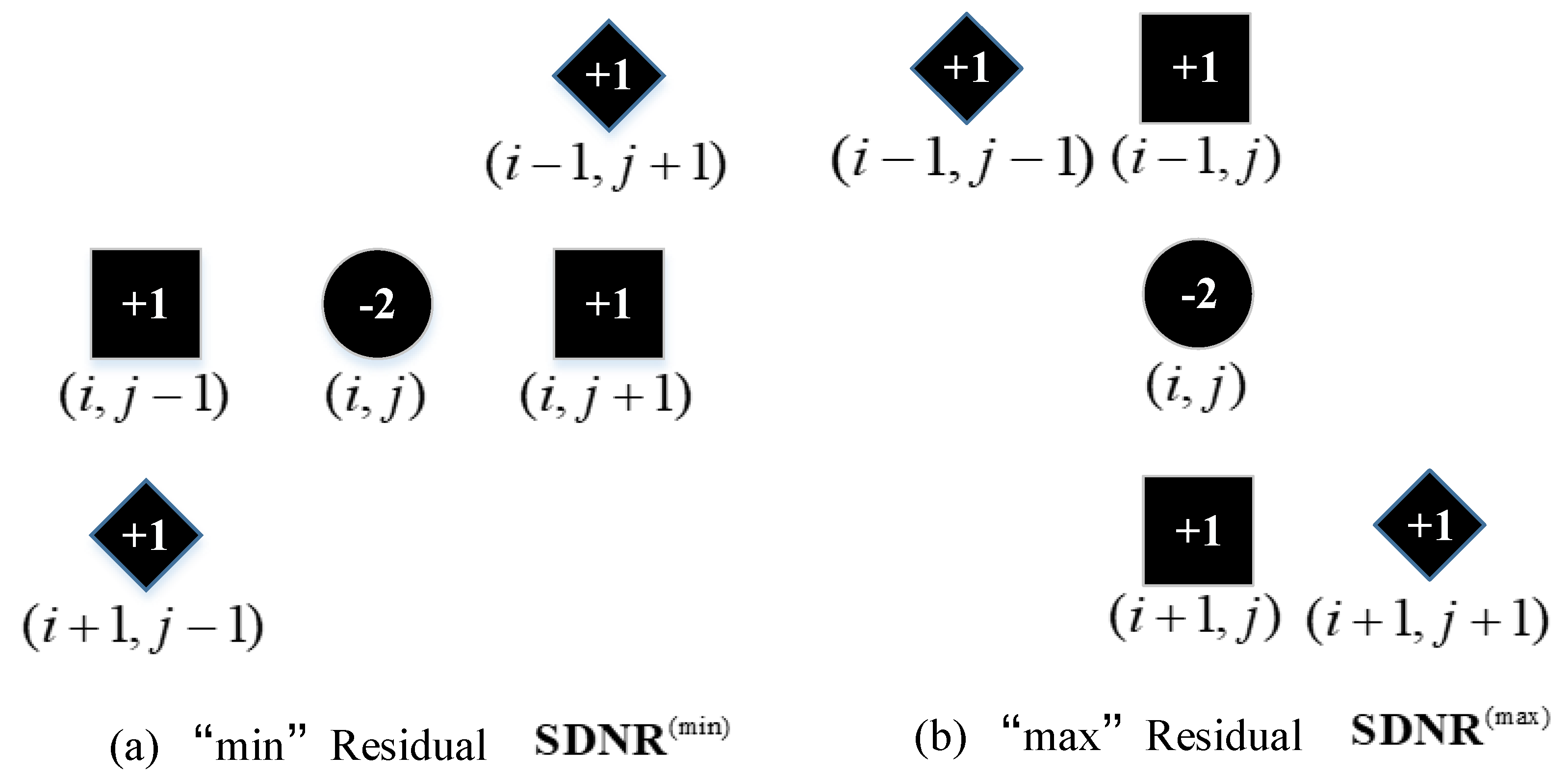
Figure 2 graphically shows the structure of the proposed SDNR, where the symbol ‘⚫’ indicates the central pixel X i , j , and the other two symbols denote the neighboring pixels and at the same time indicate the two employed filters. The SDNR can thus be formed with Equation (2).
{ S D N R i , j ( min ) = min { X i , j 1 + X i , j + 1 2 X i , j , X i 1 , j + 1 + X i + 1 , j 1 2 X i , j } S D N R i , j ( max ) = max { X i 1 , j + X i + 1 , j 2 X i , j , X i 1 , j 1 + X i + 1 , j + 1 2 X i , j }
To curb the residual’s dynamic range and make the residual more sensitive to the processing changes at the spatial discontinuities in the image, especially at the edges and textures, the quantization and truncation process are employed in the residual map S D N R { ( min ) , ( max ) } using Equation (3).
{ S N D R _ T Q i , j ( min ) = trunc T ( S N D R i , j ( min ) q + 1 2 ) S N D R _ T Q i , j ( max ) = trunc T ( S N D R i , j ( max ) q + 1 2 )
where the calculated S N D R _ T Q { ( min ) , ( max ) } means the corresponding truncated and quantized residual map; q denotes the quantization step (in our method, we set q to be the residual order, which means the absolute value of the central position coefficient of the filter); indicates the round down operation; and trunc T ( ) denotes the truncation function, which is defined in Equation (4).
trunc T ( a ) = { a ,   if   ( | a |   <   T ) T ,   if   ( | a | T )
where a is the input to this truncation function. a = S N D R i , j ( min ) q + 1 2 for residual map S D N R ( min ) and a = S N D R i , j ( max ) q + 1 2 for residual map S D N R ( max ) . Meanwhile, T denotes the truncation coefficient; in this paper, we set T = 2 , which is the same value used in [22].
Next, the horizontal co-occurrence C O d { ( min ) , ( max ) } is constructed from the four consecutive residual samples generated from Equation (3) by using Equation (5), and it is therefore a four-dimensional array.
{ C O d ( min ) = 1 Z | ( S N D R _ T Q i , j ( min ) , S N D R _ T Q i , j + 1 ( min ) , S N D R _ T Q i , j + 2 ( min ) , S N D R _ T Q i , j + 3 ( min ) ) | C O d ( max ) = 1 Z | ( S N D R _ T Q i , j ( max ) , S N D R _ T Q i , j + 1 ( max ) , S N D R _ T Q i , j + 2 ( max ) , S N D R _ T Q i , j + 3 ( max ) ) |
where d = ( d 1 , d 2 , d 3 , d 4 ) { T , T + 1 , , T 1 , T } 4 , with T = 2 and ( 2 T + 1 ) 4 = 625 , and therefore, each array has 625 elements, which gives the size of each C O ; Z denotes the normalization factor, and it is used to satisfy Equation (6).
d = ( d 1 , d 2 , d 3 , d 4 ) C O d { ( min ) , ( max ) } = 1
Considering the fact that the symmetries can increase the statistical robustness of the model while decreasing its dimensionality, we use the sign symmetry (which means that taking a negative of an image does not change its statistical properties) and the directional symmetry of the images. It can be easily seen from Figure 2 that the SDNR is directionally symmetric while it is not sign symmetric, and we propose employing Property I to achieve sign symmetry.
Property I:
For any finite set φ , min ( φ ) = max ( φ )
C O ¯ d = C O d ( min ) + C O d ( max )
C O ¯ ¯ d = C O ¯ d + C O ¯ d
where d = ( d 1 , d 2 , d 3 , d 4 ) and d = ( d 4 , d 3 , d 2 , d 1 ) ; C O ( min ) and C O ( max ) denote the “min” and “max” co-occurrence matrices in Equation (6), calculated from the same residual.
With the symmetrization process in Equations (7) and (8), which turns the “min” co-occurrence C O ( min ) and “max” co-occurrence C O ( max ) into a single matrix, the dimensionality is thus reduced from 2 × 625 to 1 × 325 . Therefore, the dimensionality of our proposed feature S D N R is 1 × 325 .

2.2. Employed Convolutional Neural Network Model for Classification

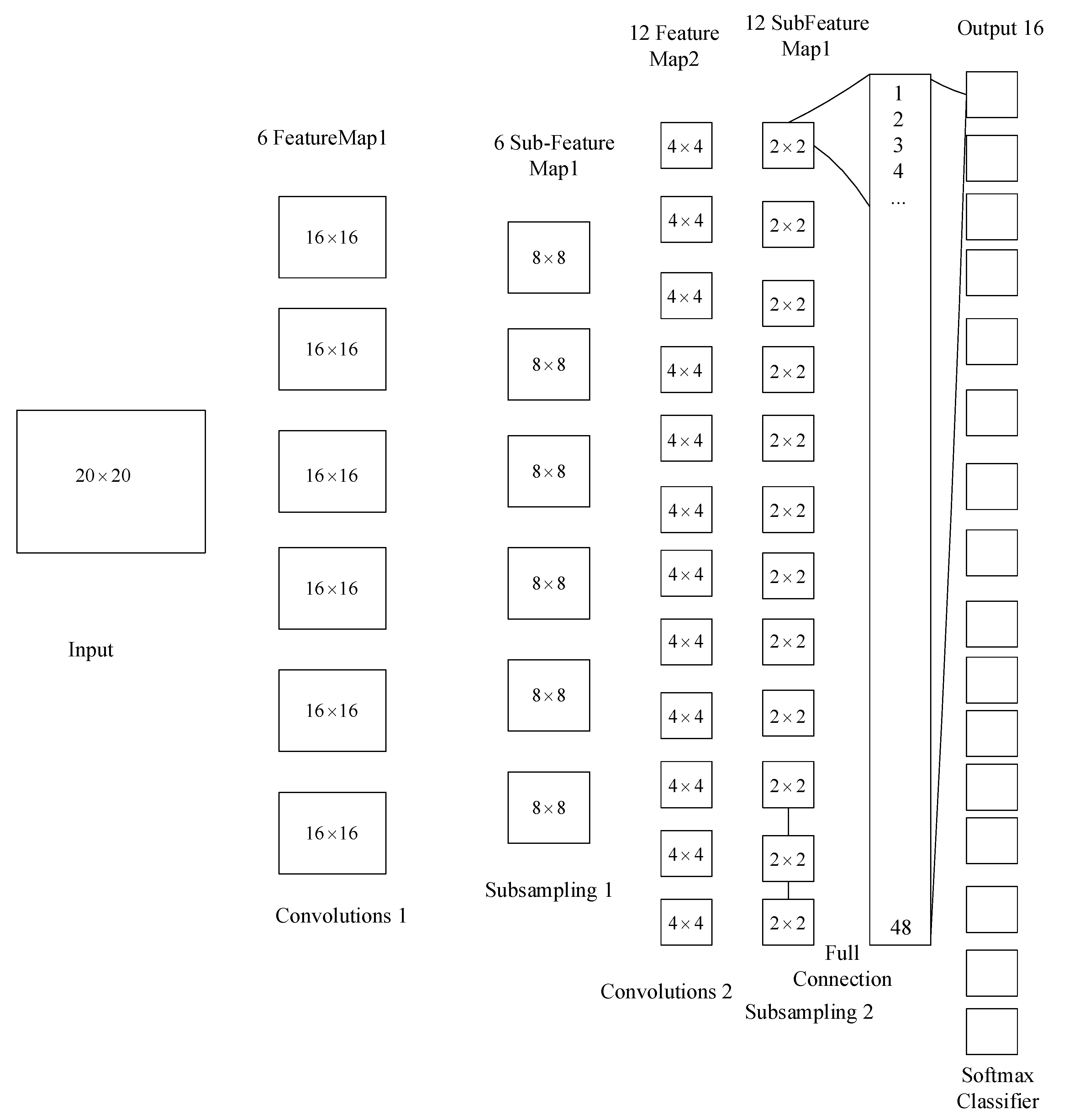
With the extracted SDNR feature, we next propose applying the five-layer CNN, as shown in Figure 3, to detect and identify a variety of image operations. The applied five-layer CNN includes two convolutional layers, two pooling layers, and one fully connected layer, followed by one softmax classifier. Compared with the conventional methods, which take pixel values as input, the proposed method improves the generalization ability and accelerates the network convergence by replacing the pixel values with extracted features. To match the feature size of 1 × 325 as explained above, we set the size of the input layer to be 20 × 20 and employ a padding operation to the extracted features. The convolutional layers aim to extract the feature maps, and each of their neurons is connected with the neighboring neuron in its former layer. As shown in Figure 3, our employed CNN model involves two convolutional layers and two pooling layers. Regarding the convolutional layers, convolutional layer 1 has six kernels with a receptive field size of 5 × 5 , and each feature map is 16 × 16 in size; while convolutional layer 2 has twelve kernels with a size of 5 × 5 , and each feature map has a size of 4 × 4 . The subsampling layer, which is an important component of the CNN model, is put between the two convolutional layers. Through reducing the connections between the two convolutional layers, the subsampling layer helps to reduce the calculation complexity. Regarding the pooling layers, both of these two layers have one kernel with a size of 2 × 2 that resamples the input spatially and reduces 75% of the activations. The down pooling methods that are frequently used are mean pooling and max pooling.
In addition to the two convolutional layers and the two subsampling layers described above, the employed CNN model involves one full connection layer that is connected with each neuron in the former layer and is followed by a softmax classifier. The full connection layer transforms the feature map extracted from the former layer into a vector with a size of 1 × 48 and feeds this vector into the softmax classifier to perform identification. Softmax regression is the promotion of a logistic regression model in problems with multiple classifications. The estimation of probability values is usually achieved through the hypothetical function h θ ( x ) in Equation (9). Given x as the input and y as the class label, we assume that the output of the function is a k-dimensional vector, which means that there are k numbers for the value of the class label y , and the sum of the vector factors in the representation of the k estimated probability values is 1.
h θ ( x i ) = ( p ( y ( i ) = 1 | x i ; θ ) p ( y ( i ) = 2 | x i ; θ ) p ( y ( i ) = k | x i ; θ ) ) = 1 j = 1 k e θ j τ x ( i ) ( e θ 1 τ x ( i ) e θ 2 τ x ( i ) e θ k τ x ( i ) )
where θ 1 , θ 2 , θ k n + 1 ; 1 j = 1 k e θ j τ x ( i ) represents the normalization of the probability distribution.
Usually, the softmax regression algorithm can be solved by minimizing the cost function; however, it has been proven that there is more than one minimization solution of the cost function of a softmax regression algorithm. To solve the multisolution phenomenon, we propose employing the method that adds a weight attenuation term into the cost function. The cost function after adding the weight attenuation term is shown in Equation (10).
J ( θ ) = 1 m [ i = 1 m j = 1 k I { y ( i ) = j } log e θ 1 τ x ( i ) j = 1 k e θ j τ x ( i ) ] e θ 1 τ x ( i ) I = 1 k e θ I τ x ( i ) + γ 2 i = 1 k j = 0 m θ i j 2
where I { } is the indicative function. When y ( i ) = j is true, I { y ( i ) = j } = 1 ; otherwise, I { y ( i ) = j } = 0 . In addition, γ denotes the weight attenuation term, and γ > 0 .
To minimize the cost function J ( θ ) , the iterative gradient descent method is used to guarantee that it converges to the optimum solution over the whole situation. The derivative function of J ( θ ) is given in Equation (11).
By minimizing the J ( θ ) , the softmax regression model can be achieved.
θ j J ( θ ) = 1 m i = 1 m [ x ( i ) ( I { y ( i ) = j } p ( y ( i ) = j | x ( i ) ; θ ) ) ] + γ θ j

3. Experiments and Discussions

In the experiments conducted to test the performance of the proposed strategy, we randomly selected a huge number of raw images from the dataset Boss Base v1.0 [29]. For each of the original images, 15 counterparts were created by applying the image processing operations with random parameters from the predefined range. Table 1 lists the 15 image operations that were tested and the predefined range of the parameters of the corresponding operations, including spatial enhancement, e.g., gamma correction (GC) and histogram equalization (HE); spatial filtering, e.g., mean filtering (MeanF) and Wiener filtering (WF); geometric operation, e.g., scaling (Sca) and rotation (Rot); lossy compression, e.g., JPEG and JPEG2000 (JP2); and frequency filtering, e.g., high-pass filtering (HPF) and homomorphic filtering (HF). All of these images were then divided into two categories randomly: half of them were utilized for training and the other half for testing.

3.1. Parameter Settings

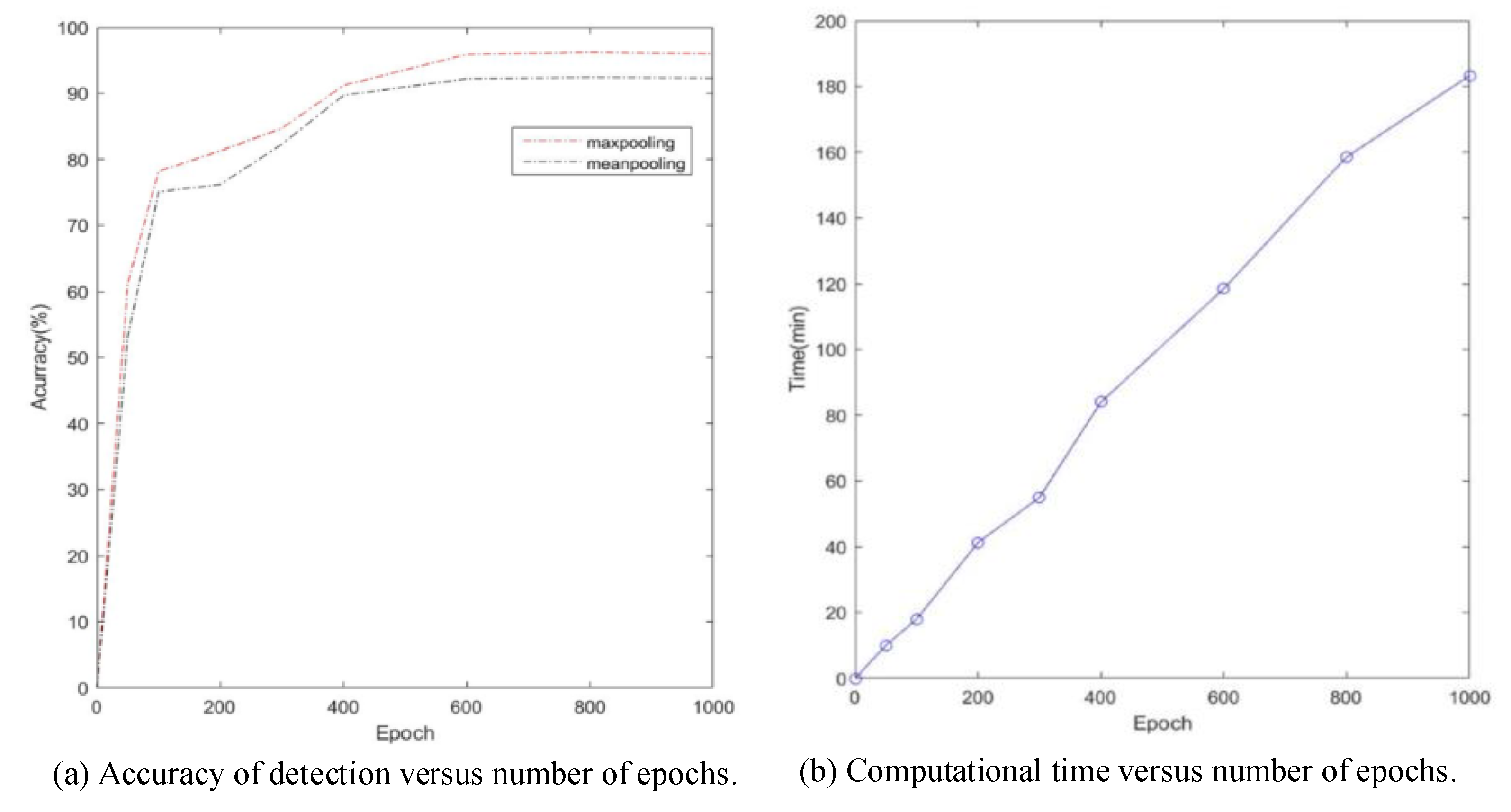
In the employed CNN architecture, the number of epochs has a large effect on the accuracy of the identification and the computational time. Therefore, in order for the proposed strategy to achieve good performance, it is important to determine how to set the appropriate parameters. Figure 4 shows the relationship between the accuracy of detection and the number of epochs (shown on the left) and the relationship between the computational time and the number of epochs (shown on the right). The results clearly indicate that either the detection accuracy or the computational expense increases with the number of epochs. To achieve a balance between the computational expense and the detection accuracy, we set the number of iterations to be 600, i.e., n u m _ e p o c h s = 600 .
As explained in Section 2.2, the pooling methods that are frequently used are mean pooling and max pooling. According to the respective results with mean pooling and max pooling, as shown in Figure 4, the max pooling always obtains a better result than the mean pooling. Therefore, we set the pooling type as max pooling in the following experiments. In addition to the number of epochs and the pooling type, the kernel size plays an important role in our method as well. By setting the number of iterations to 600, we tested the detection accuracies with different kernel sizes, 3 × 3 , 5 × 5 , and 7 × 7 , and the detection results are 92.2%, 95.9%, and 91.7%, respectively. Therefore, we set the kernel size to 5 × 5 to achieve the highest accuracy.

3.2. Detection and Classification of Various Image Postprocessing Operations

In this section, we present the results of our evaluation of the performance of the proposed method, which was conducted by measuring the accuracy of the detection and classification of the various image operations. Table 2 shows the accuracy of the detection of 15 operations using different classifiers. We applied the Ensemble classifier [24], the backpropagation neural network (BPNN) [26], the AlexNet [28], and the proposed CNN as classifiers within the proposed framework to calculate the corresponding detection accuracy. Additionally, to show the superiority of the proposed SDNR feature, we applied the subtractive pixel adjacency matrix (SPAM) [30] for comparison. It is observed that when applying the SPAM feature, the detection accuracy is 96.5% on average when using the Ensemble classifier, 94% on average when using the BPNN, 96.8% on average when using AlexNet, and 97.7% on average when using the employed CNN, while the corresponding detection accuracies are 97.1%, 95.3%, 97.5%, and 98.9%, respectively, when applying the different classifiers with the proposed SDNR. The comparison results demonstrate that the proposed SDNR feature outperforms the SPAM feature when using different classifiers. For the classifiers, the performance of the employed CNN is shown to be better than that of the other tested classifiers. In Table 2, the last row shows the average detection results with different features and classifiers and the results are highlighted in italic. The results demonstrate that the proposed approach performs very well in detecting the various image postprocessing operations.
In addition to detecting whether or not the images have been processed, this approach can also identify a variety of operations. Table 3, Table 4 and Table 5 show the confusion matrices of the multiclass identification results using the proposed SDNR feature paired with BPNN [26], AlexNet [28], and the employed CNN classifier. In Table 3, Table 4 and Table 5, the symbol ‘*’ indicates that the predicted percentage is under 0.1%, which means that the classification can be ignored. The results in the diagonal show the multiclass classification results and are highlighted in bold for easy following. According to the results, the identification accuracy is calculated as 91.3% on average with the proposed SDNR features and BPNN [26], 92.5% on average with the proposed SDNR features and AlexNet [28], and 95.9% on average with the proposed SDNR features and the employed CNN classifier. These very good results indicate the effectiveness of the proposed method.
Furthermore, in addition to the comparison of detection of various image postprocessing operations, the comparison of classification of various image postprocessing operations using different features with different classifiers is shown in Table 6. Similar to the results shown in Table 3, to show the superiority of the proposed SDNR feature, we applied the SPAM [30] for comparison, and the BPNN [26], the AlexNet [28], and the employed CNN classifier were respectively applied within the proposed framework to calculate the corresponding classification accuracy. It is observed that when applying SPAM feature, the classification accuracy is 89.7% on average when using BPNN, 90.6% on average when using AlexNet, and 85% on average when using the employed CNN, while the corresponding detection accuracies are 88.89%, 92.2%, and 95.9%, respectively, when applying the different classifiers with the proposed SDNR. The results demonstrate that the proposed method performs the best for classifying a variety of image postprocessing operations.

4. Conclusions

In summary, we have proposed the SDNR feature extraction method, which is constructed from locally supported linear filters in the spatial domain. By applying minimum and maximum operators, diversity and nonlinearity are thus introduced, and the construction thus brings nonsymmetry to the distribution of the extracted SDNR features. By applying the proposed SDNR method to the original images and the corresponding images after processing, we can extract the feature sets accordingly. This improves the acceleration of the network convergence. Then, by scanning the extracted SDNR feature sets with a patch-sized sliding window, we have proposed employing the five-layer CNN, and we trained a softmax classifier accordingly to detect and identify a variety of image postprocessing operations. The main contributions of this paper are summarized as follows: (1) We have considered the problems of both binary classification and multiclass identification in our study and solved both of them with the proposed approach. We have conducted extensive experiments on up to 15 various image postprocessing operations to evaluate the proposed approach, and the results indicate the effectiveness of our proposed method. (2) We have extracted SDNR features instead of the pixel values as the input of our deep learning model; in this way, the generalization ability can be enhanced and the network convergence can be promoted. (3) We have proposed employing the five-layer CNN as the classifier, compared with the conventional methods that use a classifier such as SVM and an ensemble classifier, to achieve higher detection accuracy. The experimental results demonstrate that the proposed approach performs well in classifying and identifying of image postprocessing operations.

Author Contributions

Data curation, T.H.; Funding acquisition, X.Y.; Investigation, X.Y.; Methodology, X.Y. and T.H.; Project administration, X.Y.; Supervision, X.Y.; Validation, T.H.; Visualization, T.H.; Writing—original draft, X.Y. and T.H.; Writing—review & editing, X.Y. All authors have read and agreed to the published version of the manuscript.

Funding

This research was funded by the National Natural Science Foundation of China, grant number 61902448.

Conflicts of Interest

The authors declare no conflict of interest.

References

  1. Fan, Z.; Queiroz, R.L.D. Identification of bitmap compression history: JPEG detection and quantizer estimation. IEEE Trans. Image Process. 2003, 12, 230–235. [Google Scholar] [PubMed] [Green Version]
  2. Farid, H. Exposing digital forgeries from JPEG ghosts. IEEE Trans. Inf. Forensics Secur. 2009, 4, 154–160. [Google Scholar] [CrossRef]
  3. Luo, W.; Huang, J.; Qiu, G. JPEG Error Analysis and Its Applications to Digital Image Forensics. IEEE Trans. Inf. Forensics Secur. 2010, 5, 480–491. [Google Scholar] [CrossRef]
  4. Bianchi, T.; Piva, A. Detection of Nonaligned Double JPEG Compression Based on Integer Periodicity Maps. IEEE Trans. Inf. Forensics Secur. 2012, 7, 842–848. [Google Scholar] [CrossRef] [Green Version]
  5. Cao, G.; Zhao, Y.; Ni, R.; Li, X. Contrast Enhancement-Based Forensics in Digital Images. IEEE Trans. Inf. Forensics Secur. 2014, 9, 515–525. [Google Scholar] [CrossRef]
  6. Stamm, M.; Liu, K.J.R. Blind forensics of contrast enhancement in digital images. In Proceedings of the 15th IEEE International Conference on Image Processing, San Diego, CA, USA, 12–15 October 2008; pp. 3112–3115. [Google Scholar]
  7. Popescu, A.C.; Farid, H. Exposing digital forgeries by detecting traces of resampling. IEEE Trans. Signal Process. 2005, 53, 758–767. [Google Scholar] [CrossRef]
  8. Mahdian, B.; Saic, S. Blind Authentication Using Periodic Properties of Interpolation. IEEE Trans. Inf. Forensics Secur. 2008, 3, 529–538. [Google Scholar] [CrossRef] [Green Version]
  9. Li, L.; Xue, J.; Tian, Z.; Zheng, N. Moment feature based forensic detection of resampled digital images. In Proceedings of the 21st ACM International Conference on Multimedia, Barcelona, Spain, October 2013; pp. 569–572. [Google Scholar]
  10. Hou, X.; Zhang, T.; Xiong, G.; Lu, Z.; Xie, K. Resampling detection aided steganalysis of heterogeneous bitmap images. J. Electron. Imaging 2013, 22, 013037. [Google Scholar] [CrossRef]
  11. Chen, C.; Ni, J.; Huang, J. Blind Detection of Median Filtering in Digital Images: A Difference Domain Based Approach. IEEE Trans. Image Process. 2013, 22, 4699–4710. [Google Scholar] [CrossRef]
  12. Kang, X.; Stamm, M.C.; Peng, A.; Liu, K.J.R. Robust median filtering forensics based on the autoregressive model of median filtered residual. In Proceedings of the 2012 Asia Pacific Signal and Information Processing Association Annual Summit and Conference, Hollywood, CA, USA, 3–6 December 2012; pp. 1–9. [Google Scholar]
  13. Kirchner, M.; Fridrich, J. On detection of median filtering in digital images. In Media Forensics and Security II; SPIE: San Jose, CA, USA, 2010; 754110. [Google Scholar]
  14. Yuan, H.D. Blind Forensics of Median Filtering in Digital Images. IEEE Trans. Inf. Forensics Secur. 2011, 6, 1335–1345. [Google Scholar] [CrossRef]
  15. Shi, Y.Q.; Chen, C.; Xuan, G.; Su, W. Steganalysis versus Splicing Detection. Digit. Watermarking 2007, 5041, 158–172. [Google Scholar]
  16. He, Z.; Lu, W.; Sun, W.; Huang, J. Digital image splicing detection based on Markov features in DCT and DWT domain. Pattern Recognit. 2012, 45, 4292–4299. [Google Scholar] [CrossRef]
  17. Zhao, X.; Wang, S.; Li, S.; Li, J. Passive Image-Splicing Detection by a 2-D Noncausal Markov Model. IEEE Trans. Circuits Syst. Video Technol. 2015, 25, 185–199. [Google Scholar] [CrossRef]
  18. Kao, H.-H.; Wen, C.-Y. An Offline Signature Verification and Forgery Detection Method Based on a Single Known Sample and an Explainable Deep Learning Approach. Appl. Sci. 2020, 10, 3716. [Google Scholar] [CrossRef]
  19. Hsu, C.-C.; Zhuang, Y.-X.; Lee, C.-Y. Deep Fake Image Detection Based on Pairwise Learning. Appl. Sci. 2020, 10, 370. [Google Scholar] [CrossRef] [Green Version]
  20. Rao, Y.; Ni, J. A deep learning approach to detection of splicing and copy-move forgeries in images. In Proceedings of the 2016 IEEE International Workshop on Information Forensics and Security, Abu Dhabi, UAE, 4–7 December 2016; pp. 1–6. [Google Scholar]
  21. Li, J.; Zhang, H.; Wan, W.; Sun, J. Two-class 3D-CNN classifiers combination for video copy detection. Multimed. Tools Appl. 2020, 79, 4749–4761. [Google Scholar] [CrossRef]
  22. Li, H.; Luo, W.; Qiu, X.; Huang, J. Identification of Various Image Operations Using Residual-based Features. IEEE Trans. Circuits Syst. Video Technol. 2016, 28, 31–45. [Google Scholar] [CrossRef]
  23. Fridrich, J.; Kodovsky, J. Rich Models for Steganalysis Digital Images. IEEE Trans. Inf. Forensics Secur. 2012, 7, 868–882. [Google Scholar] [CrossRef] [Green Version]
  24. Kodovsky, J.; Fridrich, J.; Holub, V. Ensemble Classifiers for Steganalysis of Digital Media. IEEE Trans. Inf. Forensics Secur. 2012, 7, 432–444. [Google Scholar] [CrossRef] [Green Version]
  25. Huang, T.; Yuan, X. Detection and Classification of Various Image Operations Using Deep Learning Technology. In Proceedings of the 2018 International Conference on Machine Learning and Cybernetics (ICMLC), Chengdu, China, 15–18 July 2018; pp. 50–55. [Google Scholar]
  26. Lippmann, R.P. Pattern classification using neural networks. IEEE Commun. Mag. 1989, 27, 47–50. [Google Scholar] [CrossRef]
  27. Lecun, Y.; Bottou, L.; Bengio, Y.; Haffner, P. Gradient-based learning applied to document recognition. Proc. IEEE 1998, 86, 2278–2324. [Google Scholar] [CrossRef] [Green Version]
  28. Krizhevsky, A.; Sutskever, I.; Hinton, G.E. ImageNet classification with deep convolutional neural networks. In NIPS’12: Proceedings of the 25th International Conference on Neural Information Processing Systems; Curran Associates Inc.: Red Hook, NY, USA, 2012; Volume 1, pp. 1097–1105. [Google Scholar]
  29. Bas, P.; Filler, T.; Pevný, T. Break our steganographic system: The ins and outs of organizing BOSS. In Information Hiding; IH 2011. Lecture Notes in Computer Science, Vol 6958; Filler, T., Pevný, T., Craver, S., Ker, A., Eds.; Springer: Berlin/Heidelberg, Germany, 2011; pp. 59–70. [Google Scholar]
  30. Pevny, T.; Bas, P.; Fridrich, J. Steganalysis by Subtractive Pixel Adjacency Matrix. IEEE Trans. Inf. Forensics Secur. 2010, 5, 215–224. [Google Scholar] [CrossRef] [Green Version]
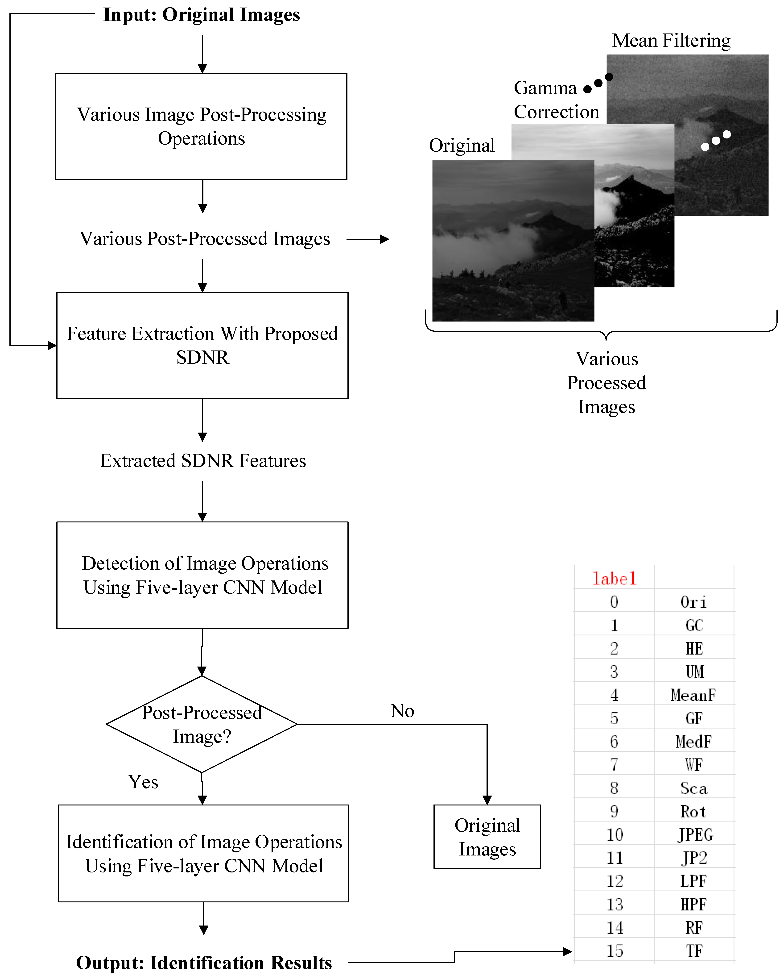
Figure 1. Framework of the proposed approach.
Applsci 10 05582 g001
Figure 2. Definition of the proposed spatial domain-based nonlinear residual (SDNR).
Applsci 10 05582 g002
Figure 3. Architecture of the employed convolutional neural network (CNN).
Applsci 10 05582 g003
Figure 4. Parameter setting for the number of epochs.
Applsci 10 05582 g004
Table 1. Tested operation types and the corresponding parameter settings.
Operation CategoriesOperation TypeParameter Setting
Spatial enhancementGamma Correction (GC)γ: 1.0, 1.6, 1.8, 2.0
Histogram Equalization (HE)n/a
Unsharp Masking Sharpening (UM)σ: 0.5–1.5
τ: 0.5–1.5
Spatial filteringMean Filtering (MeanF)Window sizes: 3 × 3, 5 × 5, 7 × 7
Gaussian Filtering (GF)Window sizes: 3 × 3, 5 × 5, 7 × 7
σ: 0.8–1.6
Median Filtering (MedF)Windows size: 3 × 3, 5 × 5, 7 × 7
Wiener Filtering (WF)Windows size: 3 × 3, 5 × 5, 7 × 7
ScalingScaling (Sca)Down-sampling: 40%, 50%, 70%
RotationRotation (Rot)Angle: 30°, 35°, 40°, 45°
Lossy compressionJPEGQuality factor: 80–90
JPEG2000 (JP2)Compression ratio: 4.0–6.0
Frequency filteringLow-Pass Filtering (LPF)Cutoff frequency: 80 Hz
High-Pass Filtering (HPF)Cutoff frequency: 30 Hz
Band-Stop Filtering (BF)Stop band: 35–65 Hz
Homomorphic Filtering (HF)n/a
Table 2. Detection of various image postprocessing operations using different features with different classifiers (%).
ClassifierEnsemble Classifier [24]BPNN
[26]
AlexNet
[28]
Employed CNN
FeatureSPAM [30]Proposed SDNRSPAM [30]Proposed SDNRSPAM [30]Proposed SDNRSPAM [30]Proposed SDNR
GC96.296.492.193.195.396.796.597.6
HE98.398.194.398.997.296.498.499.5
UM97.298.396.496.298.698.797.699.3
MeanF96.597.596.297.697.397.598.598.8
MedF97.998.197.698.897.697.197.399.6
WF98.899.696.297.198.596.597.197.6
GF99.298.797.398.398.398.89999.8
SCA91.393.490.389.192.297.595.399.5
ROT97.296.394.595.697.698.698.398.9
JPEG95.39696.897.498.599.297.898.2
JP297.497.897.696.998.798.998.198.3
LPF96.397.397.397.297.898.898.799.6
HPF98.298.196.398.396.397.897.699.7
BF93.395.384.286.794.695.697.298.2
HF94.295.682.388.693.294.39899
Average96.597.19495.396.897.597.798.9
Table 3. Identification of various image postprocessing operations using the proposed SDNR features and BPNN [26] (%).
Actual/PredictedOrigGCHEUMRotScaMeanFMedFWFGFJPEGJP2LPFHPFHFBF
Orig90.30.4*********1.63.31.6**
GC282.92.41.40.8**0.4**0.80.8****
HE*0.299.30.3***0.10.2*******
UM2.11.40.393.3***0.40.3**1****
Rot2.21.4**94.10.5******2*2*
Sca30.56.5*0.4*60.2****7.7*0.53*3
MeanF0.3*****98.8*****0***
MedF**0.8*0.40.4*97.7***0.2***0.2
WF********99.2*******
GF1****0.4***99.92*****
JPEG*0.4*0.4*0.4*0.40.4*92.50.80.50.221
JP210.4***0.4*0.4**2.487.4*0.2**
LPF0.3***********98.6***
HPF0.20.1*****0.1*0.2**0.198.40.1*
HF20.7****3.20.50.72.50.3*2.5**70.73*
BF30.510.74.215**0.5***3.5**1.659.4
Note: symbol ‘*’ indicates that the predicted percentage is under 0.1%.
Table 4. Identification of various image postprocessing operations using the proposed SDNR features and AlexNet [28] (%).
Actual/PredictedOrigGCHEUMRotScaMeanFMedFWFGFJPEGJP2LPFHPFHFBF
Orig87.50.4*********2.4*1.6**
GC292.92.41.40.8**0.4**0.80.8****
HE*0.298.70.3***0.10.2*******
UM3.21.40.393.5***0.40.3**1****
Rot1.51.4**92.20.5******2*2*
Sca1.5**0.4*87.8******0.53*3
MeanF0.3*****99.7*****0***
MedF**0.8*0.40.4*97.1***0.2***0.2
WF********99.6*******
GF1****0.4***94.82*****
JPEG*0.4*0.4*0.4*0.40.4*88.50.80.50.221
JP210.4***0.4*0.4**2.489.7*0.2**
LPF0.3***********97.5***
HPF0.20.1*****0.1*0.2**0.198.20.1*
HF0.5****10.50.72.50.3****82.2*
BF1.10.8*1***0.5******1.681.1
Note: symbol ‘*’ indicates that the predicted percentage is under 0.1%.
Table 5. Identification of various image postprocessing operations using the proposed SDNR features and the employed CNN classifier (%).
Actual/PredictedOrigGCHEUMRotScaMeanFMedFWFGFJPEGJP2LPFHPFHFBF
Orig94.60.4*********2.4*1.6**
GC293.72.41.40.8**0.4**0.80.8****
HE*0.299.10.3***0.10.2*******
UM3.21.40.393.2***0.40.3**1****
Rot1.51.4**93.30.5******2*2*
Sca1.5**0.4*92.8******0.53*3
MeanF0.3*****99.7*****0***
MedF**0.8*0.40.4*98***0.2***0.2
WF********100*******
GF1****0.4***96.62*****
JPEG*0.4*0.4*0.4*0.40.4*92.50.80.50.221
JP210.4***0.4*0.4**2.492.5*0.2**
LPF0.3***********99.7***
HPF0.20.1*****0.1*0.2**0.199.20.1*
HF0.5****10.50.72.50.3****95.3*
BF1.10.8*1***0.5******1.694.6
Note: symbol ‘*’ indicates that the predicted percentage is under 0.1%.
Table 6. Comparison of identification of image postprocessing operations using different features with different classifiers (%).
ClassifierBPNN [26]AlexNet [28]The Employed CNN Classifier
FeatureSPAM [30]Proposed SDNRSPAM [30]Proposed SDNRSPAM [30]Proposed SDNR
ORI81.1%90.3%82.3%87.5%91.4%94.6%
GC82.1%82.9%91.3%92.9%87.5%93.7%
HE94.3%99.3%93.2%98.7%94.4%99.1%
UM96.4%93.3%91.6%93.5%69.1%93.2%
MeanF96.2%97.6%97.3%99.7%89.5%95.0%
MedF97.6%98.8%94.6%97.1%77.6%98.7%
WF96.2%99.7%96.5%99.6%92.1%100%
GF97.3%99.2%93.3%94.8%91.3%99.4%
SCA90.3%60.2%70.2%87.8%90.1%92.8%
ROT94.5%94.1%92.6%92.2%92.3%93.3%
JPEG96.8%92.5%91.5%88.5%80.4%92.5%
JP297.6%87.4%89.7%89.7%89.9&92.5%
LPF97.3%98.6%97.8%97.5%80.6%99.7%
HPF82.3%98.3%86.3%98.2%89.9%99.2%
HF64.2%59.4%84.6%82.2%61.1%95.3%
BF71.3%70.7%88.2%81.1%88.1%94.6%
Average89.7%88.89%90.6%92.2%85%95.9%