A Multi-Objective Train Operational Plan Optimization Approach for Adding Additional Trains on a High-Speed Railway Corridor in Peak Periods

Abstract

Passenger demand for railway transportation rapidly increases in peak periods, and the transport capacity for existing trains is not sufficient. Railway companies usually adopt the strategy of adding additional trains in peak periods to meet the higher passenger demand. Designing a good operational plan for additional trains becomes a challenge for operators, though. A new optimization approach for designing an operational plan for additional trains is proposed in this paper. The number of trains, the operational plan, the stop plan, and the timetable for each train can be considered simultaneously in the new optimization approach, which will make it easier to design an operational plan for additional trains. A multi-objective nonlinear model with three objectives of minimizing total running distance, dwelling time, and unsatisfied passengers is proposed. Big-M is introduced to transform the nonlinear model into a linear model. The solver CPLEX is used to solve the transformed linear model and obtain the optimal operational plan. Small-scale numerical experiments are implemented to show the effectiveness of the optimization approach. The large-scale case of the Beijing‒Shanghai railway corridor is studied to demonstrate that the optimization approach can be applied to real-word and large-scale situations.

1. Introduction

1.1. Background and Motivation

Railways have become a more and more important mode of transportation in China because of advantages like safety, green potential, convenience, etc. Passenger demand is growing year by year. The number of passengers in China was 3.38 billion in 2018, an increase of 9.4% compared to 2017 [1]. For example, in just the 40 days of the spring festival, the number of passengers taking trains to travel was 0.38 billion, which was a great challenge for railway companies. These special periods are called peak periods, and others are called off-peak periods. Transport capacity is not always enough to meet passenger demand in peak periods. The purpose of this research is to look for solutions to the shortage of transport capacity in peak periods. Railway companies usually adopt the strategy of adding additional trains to deal with the shortage of transport capacity in peak periods and meet passenger demand. These trains added in peak periods are called additional trains; the trains in off-peak periods are called existing trains. Thus, a railway company must design an operational plan for additional trains in advance. There are some important indexes for evaluating the operational plan, e.g., the satisfaction of passenger demand and the operational cost. The purpose of this study is to design an efficient operational plan for additional trains that maximizes the satisfaction of passenger demand and minimizes operating costs.

In China, tickets are booked 30 days in advance. Passengers must board trains according to the information on the tickets. Tickets show the train number, price, departure time, and stations for getting on and off. Thus, the number of additional trains, operational zone, stop plan, and timetable for each additional train must be scheduled in advance. The number of additional trains is a complicated issue for a railway company. Too many additional trains will increase the operating costs, but too few additional trains cannot meet passenger demand. The operational zone specifies the origin and terminal stations for the additional train. The stop plan determines whether the train stops at the station in the operational zone. The timetable determines the departure and arrival times of each train for each station in its operational zone. Passenger distribution determines the number of passengers for each origin‒destination (OD) pair on each train. The number of additional trains, operational zones, stop plans, timetables, and passenger distribution are the key elements of the operational plan for additional trains and are related to each other. Thus, the numbers of trains, operational zones, stop plans, timetables, and the passenger demand for additional trains are jointly optimized in this paper. Specifically, the purpose of this paper is to design an operational plan, including the number of trains, operational zones, stop plans, timetables, and passenger demand, for additional trains in peak periods. In this paper, the operational zones, timetables, and stop plans for existing trains are fixed, and the operation of additional trains cannot disturb the operation of existing trains. Passengers are accustomed to the timetables and stop plans of existing trains. Frequent changes in operational zones, timetables, and stop plans for existing trains cause inconvenience for passengers. The railway corridor is a part of the railway system, and a change in the operational plan for existing trains can disturb the whole railway system. However, passenger distribution for existing trains is reoptimized to make full use of the capacity of existing trains, which is not fully utilized in the off-peak period.

1.2. Literature Review

In this section, some studies related to the study are surveyed. The following three related problems are discussed in this section: the problem of adding additional trains, line planning problems (LPPs), and train timetable problems (TTPs). A practical problem solved in our work is that of adding additional trains. Meanwhile, we aim to design the operation zone, the number of trains, and timetable etc. Two related classic problems, i.e., LPP and TTP, are discussed in this section.

The problem of adding trains is an emerging problem that some researchers have begun to address. Researchers [2,3,4] studied the problem of adding additional trains. Burdett and Kozan [2] considered the problem of adding additional trains as a job shop problem and presented a constructive algorithm and simulated annealing approach to solve the model. Cacchiani and Caprara [3] studied the problem of inserting additional freight trains into the timetables of existing passenger trains. Gao et al. [4] focused on the problem of adding passenger trains on a high-speed railway corridor, wherein the timetables of existing trains can be modified. Although researchers focused on the problem of adding additional trains, there are still several issues that have not been considered in the literature. First, the number of additional trains was not considered. In most cases of adding trains, more additional trains are better, but researchers have not determined the ideal number of additional trains to save on operating costs and meet passenger demand. Second, the timetables of additional trains, operational zone, stop plan, etc. have not been considered in the literature. Third, passenger demands were ignored in the models of the above studies. The purpose of adding additional trains is to meet passenger or freight demand, so passenger demand is a very important element of the problem of adding additional trains. Liu et al. [5] presented a bi-objective integer programming model to solve the problem of adding additional trains in a high-speed railway corridor in peak periods. The number of trains, stop plans, train types, and timetables for additional trains were designated in the model, in which passenger demand was also considered. However, several problems have not been considered in the above studies. OD passenger demands have not been considered. Although passenger demand was discussed by Liu et al. [5], the number of passengers who get on and off was not tackled. Obviously, OD passenger demand is more accurate than a macroscopic view. The other issue is that the operational zone was not considered. These gaps are addressed herein.

The problem of adding trains falls into the scope of railway operations. One related problem is the LPP. LPP involves designing a line system such that travel demand is satisfied and certain objectives are met [6]. Most researchers studied LPP, determining the operational zone and number of trains for each zone without consideration of a timetable [7,8,9,10,11,12]. Researchers studying TTP focus on the timetables of trains. TTP is very popular in the area of railway operations, and numerous researchers have given it attention [13,14,15,16,17,18,19]. Recently, passenger demand has become an important factor considered by researchers on TTP [20,21,22,23,24]. Some researchers on LPP paid attention to passenger demand [25,26,27,28]. Specifically, Sperry and Nie [25] introduced a passenger flow assignment product to determine the stop plan under a given operational zone and the frequency for each. A similar passenger flow assignment method is introduced by Qi et al. [27] and Qi et al. [28]. The passenger flow assignment method is referred to in this paper to cope with passenger distribution when adding additional trains. Whether LLP or TTP, most researchers have considered either the operational zone and the number of trains or the timetable. This paper represents a combination of those approaches and jointly optimizes the operational zones, number of trains, and timetables for additional trains.

1.3. Contribution

The main contributions of this paper are summarized as follows:

First, we propose a new optimization method for designing an operational plan for additional trains. In the optimization method, the number of trains, operational zone, stop plan, timetable, and passenger distribution are jointly optimized. Additional trains are added occasionally based on passenger demand in peak periods, and the decision making about them is made in a short time horizon.

Second, a multi-objective nonlinear programming model for designing an operational plan is proposed for additional trains on the high-speed railway corridor. There are three objectives in the model, wherein the operational cost and passenger service are considered simultaneously. Adding additional trains aims to meet the passenger demand in peak periods. Thus, minimizing unsatisfied passenger demand is one of the objectives. However, the operating cost is also a concern for a railway company. In the model, running distances of trains are selected as an index of operating costs. Minimizing dwelling time is one of the objectives of the optimization model. In addition, we introduced the big-$M$ method to transform the nonlinear model into the linear model, which is easier to solve with a CPLEX solver.

Third, a set of small-scale numerical experiments are implemented on a small railway corridor, including six stations, and a large-scale case on the Beijing‒Shanghai railway corridor is also studied. The results of these numerical experiments demonstrate the good performance of the proposed optimization method.

The remainder of this paper is organized as follows: In Section 2, we provide a detailed problem description. In Section 3, we present the assumptions and a multi-objective integer programming model for designing an operational plan for additional trains. Two techniques for solving the model are introduced in Section 4. In Section 5, we conduct a series of small-scale experiments and a large-scale experiment to evaluate the performance of the proposed approach. In Section 6, the conclusions of this study are presented, and future work is discussed.

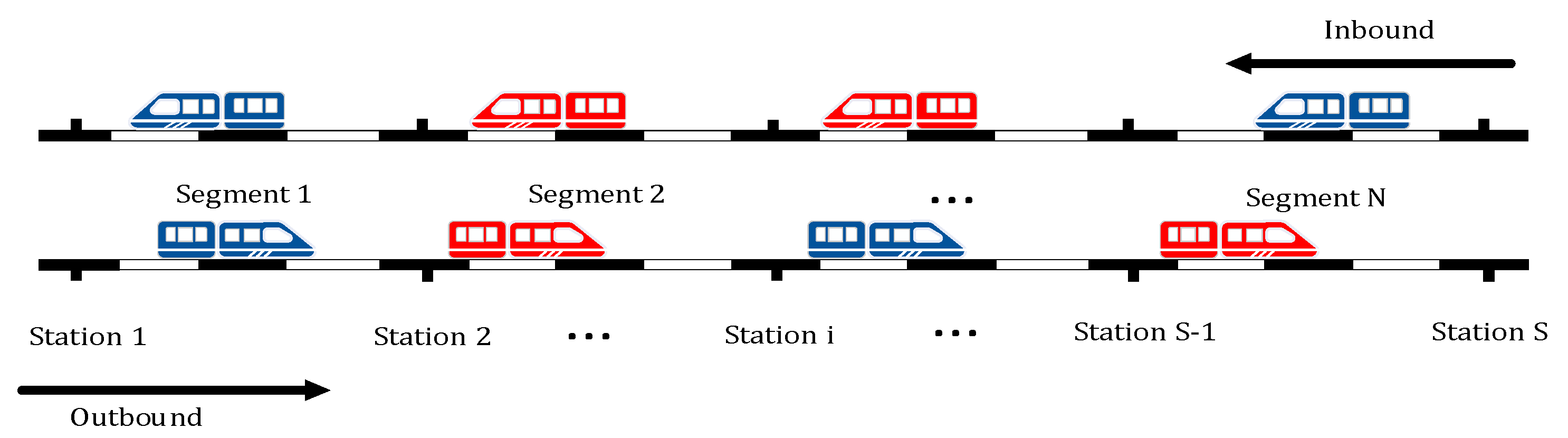
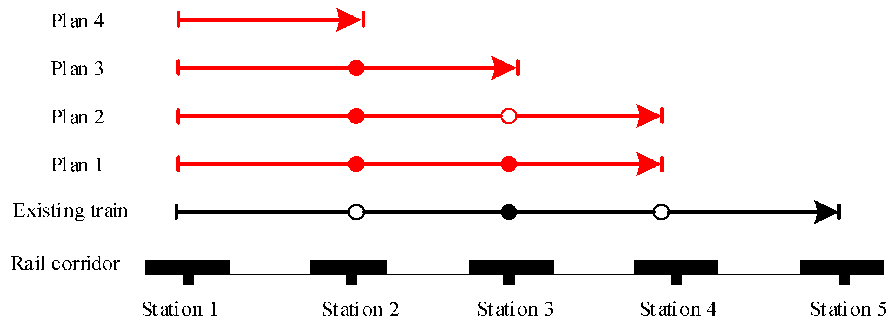
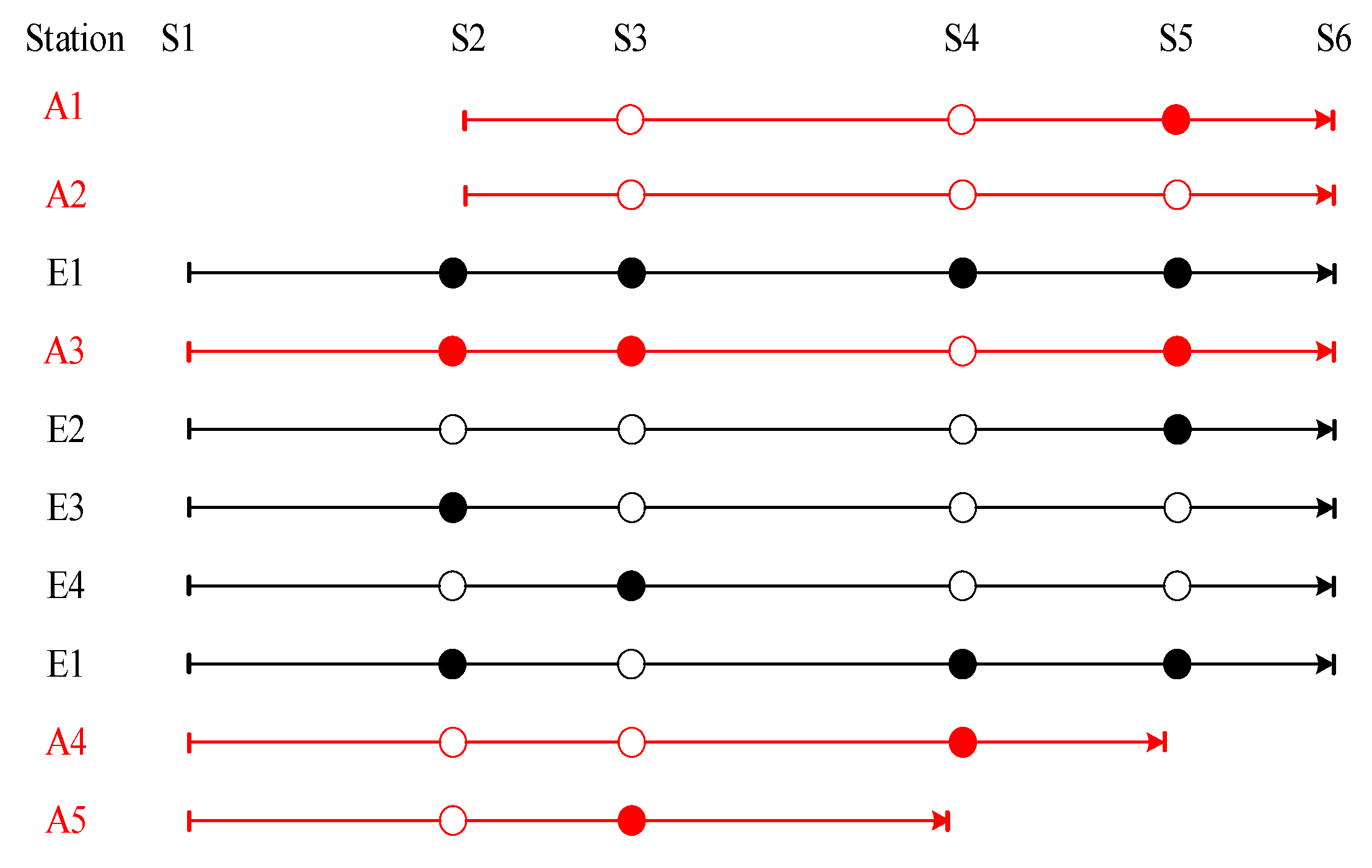
2. Problem Description

In this section, a detailed description of the problem and assumptions is given. A railway corridor consists of a set of stations and segments that connect two consecutive stations. Figure 1 shows a double-track railway corridor from station 1 to station $S$. The segments between two consecutive stations are indexed as $\left\{1 , 2 ,\dots ,N\right\}$. Since the study environment is a high-speed railway corridor, which is always double-track, we only consider our problem on the outbound-track railway corridor. For the outbound railway corridor, station 1 is the starting station of the railway corridor and station $S$ is the ending station. The starting station of the railway corridor can only be selected as the origin station of an outbound trip, and the ending station can only be selected as the terminal station of a trip. There are two sets of trains ($K_1\cup K_2$) in this problem, wherein $K_1$ is the set of existing trains and $K_2$ is the set of additional trains. In peak periods, existing trains cannot meet the passenger demand. As shown in Figure 1, the blue trains represent existing trains in the off-peak period. To provide more transport capacity, we will insert some additional trains—the red trains in Figure 1.

Our goal is to design an operational plan for additional trains. The operational plan includes the number of trains, operational zones, stop plans, timetables, and passenger distribution for trains. The reason why all plans for the number of trains, operational zones, stop plans, timetables, and passenger distribution are jointly optimized is that these plans are closely connected. In the following, we will explain the connection between them.

A small example is shown in Figure 2 to illustrate the impact of the operational zone and stop plans on the distribution of passenger demand. As shown in Figure 2, a railway corridor with five stations and four segments is considered. In Figure 2, there are five lines with arrows to represent the operational plans for trains. The arrows indicate the running direction of the train. The endpoint of a line represents the origin station or terminal station. A solid dot in the line denotes the train stopping and a hollow dot denotes a non-stopping train. The black line represents the operational plan for the existing train. The red lines represent four potential operational plans for the additional train. We assume only one existing train runs on this corridor, and the operational zone is from station 1 to station 5 in this example. The capacity of each train is$N$. The passenger demand for each OD pair is listed in

Table 1. Passenger demand for each origin‒destination (OD) pair.

Origin/Terminal Station	1	2	3	4	5
1		N	N
2				N
3					N

. In Table 1, $N$ denotes that $N$ passengers want to travel from their origin station to the terminal station. Obviously, the best stopping plan for the existing train is to stop at station 3. $N$ passengers take the existing train to travel from station 1 to station 3, then another $N$ passengers take it to travel from station 3 to station 5. However, the existing train still cannot meet the passenger demand, so adding an additional train is necessary. Four potential plans for the additional train are considered, as shown in Figure 2. We compare these different plans for the additional train. Several indexes of these plans are summarized in

Table 2. The comparison of plan 1, plan 2, plan 3, and plan 4.

Operation Zone	Operational Cost	Loading Passengers	Unsatisfied Passenger Demand
Off-peak	$E$	$2N$	$2N$
Plan 1	$E+3c+2s$	$3N$	$N$
Plan 2	$E+3c+\mathrm{s}$	$4N$	0
Plan 3	$E+2c+\mathrm{s}$	$2.5N$	$0.5N$
Plan 4	$E+c$	$3N$	$N$

. We set the operating cost of the existing trains to $E$, because the operational zone and stop plan for the existing train are fixed. In this example, we assume that the operating cost of additional trains is related to the number of segments of their operational zone and the number of stops. The operational cost of each segment is $c$, and the operational cost of each stop is $s$. First, we compare plan 1 and plan 2, which demonstrate the impact of the stop plan on the distribution of passenger demand and operating cost. As shown in Figure 2, plan 1 and plan 2 have the same operational zone from station 1 to station 4 but different stop plans. In Plan 1, the additional train stops at station 2 and station 3, while the train in plan 2 just stops at station 2 and skips station 3. We assume that when passengers have two choices of ways to reach their destination, we can distribute the passengers equally to each train. If we adopt plan 1, passengers going from station 1 to station 3 have two choices, which means that $N/2$ passengers take existing trains to station 3 and $N/2$ passengers take the additional trains in plan 1 to station 3. Meanwhile, only $N/2$ passengers going from station 1 to station 2 can board the train at station 1. Then, passengers from station 1 to station 2 get off at station 2, and the rest of the capacity of the additional train at station 2 is $N/2$, which results in only $N/2$ passengers boarding the train to go from station 2 to station 4. In consequence, $N/2$ passengers going from station 2 to station 4 cannot get to their destination, and $N/2$ seats are empty in the existing train from station 1 to station 3. Passengers from station 1 to station 3 cannot take the additional train in plan 2 because the train does not stop at station 3. $N$ passengers take the additional train in plan 2 from station 1 to station 2, then $N$ passengers take this train from station 3 to station 5 to get their destination. It is known from Table 2 that, although the operating cost of plan 1 is higher than that of plan 2, the number of unsatisfied passengers is greater. Another comparison between plan 3 and plan 4 is implemented. We know from Figure 2 that the operational zone in plan 3 is longer than that in plan 4. However, there are $N/2$ passengers going from station 1 to station 2 who can board the additional train in plan 3 because passengers going from station 1 to station 3 can reach their destination. Meanwhile, there are $N$ passengers who can take the additional train from station 1 to station 2 in plan 2. As listed in Table 2, although the operational zone in plan 3 covers more segments and stations, both the unstratified demand and the operating cost are higher than in plan 4. The two comparisons show that more stops and a longer operational zone do not always load more passengers and may cause more empty seats and higher operating costs. This example illustrates the necessity of the optimization of the operational zone and stop plan for additional trains, which can improve passenger satisfaction, cost-saving, and utilization of transport capacity.

However, we cannot ignore the importance of optimizing timetables for additional trains. The timetable has a great impact on the operational zone, stop plan, and passenger distribution. The departure and arrival times of additional trains must maintain the time interval between additional and existing trains; we call that time interval headway because the added train must avoid conflicting with existing trains and additional trains. In a finite time horizon, the number of trains that can be added is finite because of headway.

3. Formulation

In this section, we formulate a mathematical model to design the operational plan for additional trains in peak periods. The parameters in the model are listed in

Table 3. Parameters.

Notions	Definitions
$S=\left\{1, 2,\cdots ,\left|S\right|\right\}$	Set of stations
$T_s$	The set of traveling time of segments.
$K_1=\left\{1, 2,\cdots , \left|K_1\right|\right\}$	The set of existing trains
$K_2=\left\{1, 2,\cdots , \left|K_2\right|\right\}$	The set of expected additional trains
$\left[1, T\right]$	The time window of additional train arrives at its terminal station
$i,j$	The index of station, $i,j$ $\in$ $S$.
$\left(i,j\right)$	The index of OD pair, $i,j$ $\in$ $S$.
$\left(i,i+1\right)$	The index of segment on the railway corridor, $i\in S/\left\{\left|S\right|\right\}$
$t_{i,i+1}$	The traveling time of train on the segment $\left(i,i+1\right)$
$L_i$	The distance from station$i$to station 1
$k$	The index of train, $k\in K_1\cup K_2$
$h_{min}$	The minimum headway of trains
$d_{min}$	The minimum dwelling time
$d_{max}$	The maximum dwelling time
$D_{i,k}^e$	The departure time of existing train $k$ at station $i, k\in K_1$, $s\in S$.
$A_{i,k}^e$	The arrival time of existing train $k$ at station $i, k\in K_1$,$s\in S$.
$z_{ki}^{eI}$	Indicator for station $i\in S$ as origin station of existing train $k\in K_1$ for:$=1$ if train $k$ select station $i$ as its origin station, = 0 otherwise.
$z_{ki}^{eT}$	Indicator for station $i\in S$ as terminal station for existing train $k\in K_1$:$=1$ if train $k$ select station $i$ as its origin station, = 0 otherwise.
$y_{ki}^e$	Indicator for existing train $k\in K_1$ stopping at station $i\in S$:$=1$ if train $k$ stop at station $i$, = 0 otherwise.
$C_k$	The maximum loading capacity of train$k$
$y_{min}$	The required minimum number of boarding and alighting passengers for train stopping.
$Q_{ij}$	Passenger demand for OD pair $\left(i,j\right)$
$Q_{max}$	The total outbound passenger demand along the whole railway corridor
$N_{K_1}$	The number of existing trains
$N_{K_2}^e$	The expected number of additional trains
$N_{K_2}$	The number of additional trains

, and decision variables are listed in

Table 4. Decision variables.

Variables	Definitions
$x_k$	selection indicator for adding additional train $k\in K_2$:$=1$ if train $k$ is added in peak period,$=0$ otherwise;
${\mu }_{kf}^i$	selection indicator for the departure order of train $k\in K_{2 }$and train $f\in K_{1 }\cup K_2$ at station $i$.=1 if train $k$ depart from station earlier than train $f$ before, =0 otherwise.
$y_{ki}$	selection indicator for stop plan for additional train $k\in K_2$ for station $i\in S$:=1 if train $k$ stop at station $i$, $=0$ otherwise.
$z_{ki}^I$	selection indicator for origin station for additional train $k\in K_2$ for station $i\in S/\left\{\left|S\right|\right\}$:$=1$ if train $k$ select train $i\in S/\left\{S\right\}$ as its origin station, = 0 otherwise.
$z_{ki}^T$	selection indicator for terminal station additional train $k\in K_2$ for station $i\in i\in S/\left\{1\right\}$:$=1$ if train $k$ select train $i$ as its terminal station, = 0 otherwise;
$D_{ki}^a$	departure time of train $k$at station $i$, where $k\in K_2$and $i\in S/\left\{\left|S\right|\right\}$.
$A_{ki}^a$	arrival time of train $k$ at station$i$, where $k\in K_2$and $i\in S_I\cup S/\left\{1\right\}$
$q_{ij}^k$	the number of passengers take additional train $k$ from station $i$ to station $j$,$k\in K_2, i,j\in S$.
${\rho }_{ij}^{’k}$	the number of passengers take existing train $k$ from station $i$ to station $j$ in peak period,$k\in K_1, i,j\in S$.

. First, some assumptions are listed to simplify the problem.

• The traveling time of each segment is fixed.
• The capacity of the station and the rolling stocks is unlimited.
• Dwelling time at the origin station and terminal station of the trip for each train is not considered.
• The difference between the infrastructure of stations is not considered. In the real word, the infrastructure in some small-scale stations is so poor that they are not suitable to serve as an origin station or terminal station. In this paper, we assume that all stations are qualified to serve as an origin station or terminal station for additional trains.

3.1. Decision Variables

There are two types of decision variables in the model—binary variable and integer variable. The first binary variable $x_k$ is used to determine whether additional train $k$ is added to the operational plan in the peak period. We use the binary variable ${\mu }_{kf}^i$ to determine the departure order of trains, which indicates the overtaking of trains at stations. Binary variable $y_{ki}$ indicates the stop plan for the train. Another two binary variables, $z_{ki}^I$ and $z_{ki}^T$, are used to determine the operational zone for train $k$. $D_{ki}^a$ and $D_{ki}^a$ are two integer variables to determine the timetables for additional trains. $q_{ij}^k$ is the integer variable to indicate the distribution of passenger demand of each OD pair along the railway corridor.

It is worth mentioning that the value of decision variable $x_k$ determines the number of additional trains. $N_{K_2}^e$ denotes the number of expected additional trains, and we set the value of $N_{K_2}^e$ according to Equation (1). $\sum _{i^{\prime }\le i,j>i}{Q}_{i^{\prime }j} /C_k$ represents the required number of trains to meet the passenger demand along segment $\left(i,i+1\right)$. The maximum required number among all segments is the expected additional trains. However, not all of the additional trains can be added into the operational plan because it is subject to limited transport resources in peak periods. The value of decision variable $x_k$ is equal to 1, which means train$k$ is added to the operational plan. Otherwise, train $k$ is canceled. Thus, the number of additional trains $N_{K_2}$ in the operational plan is equal to the value of $\sum _{k\in K_2}{x}_k$, as in Equation (2).

$$N_{K_2}^e=ma{x}_{i\in S}\left\{{\displaystyle \sum }_{i^{\prime }\le i,j>i}{Q}_{i^{\prime }j} /C_k-N_{K_1}\right\}$$

(1)

$$N_{K_2}={\displaystyle \sum }_{k\in K_2}{x}_k$$

(2)

3.2. Formulations of Constraints

3.2.1. Constraints of Operational Zone

Not all added additional trains need to travel across the whole rail corridor. Designing the operational zone requires selecting the origin station and terminal station for additional trains. Formulating some constraints to design the appropriate operational zones for the added trains makes sense. First, it is known that only one origin station and terminal station exists during an additional train’s one trip. Constraint (3) is formulated to restrict that, as follows, i.e.,

$${\displaystyle \sum }_{i\in S}{z}_{ki}^I={\displaystyle \sum }_{ i\in S}{z}_{ki}^T=x_k k\in K_2. \left(3\right)$$

(3)

Since the index of terminal station must be after the origin station, we formulate Constraint (4): if station $i$ is selected as the origin station for train $k$, all the stations before $i$ cannot be selected as the terminal station for train $k$. Similarly, Constraint (5) indicates that station $i$ is selected as the terminal station for train $k,$ which means that all stations after $i$ cannot be the origin station for train$k$.

$${\displaystyle \sum }_{i^{\prime }\in S,i^{’}\le i}{z}_{k{i}^{\prime }}^T\ast z_{ki}^I\le 0 k\in K_2 , i\in S.$$

(4)

$${\displaystyle \sum }_{i^{\prime }\in S,i^{’}\ge i}{z}_{k{i}^{\prime }}^I\ast z_{ki}^T\le 0 k\in K_2 , i\in S.$$

(5)

For an outbound trip, the starting station of the railway corridor is not set as the terminal station and the ending station of the railway corridor cannot be the origin station. Thus, we formulate Constraint (6) as follows, i.e.,

$${\displaystyle \sum }_{k\in K_2}{z}_{k\left|S\right|}^I={\displaystyle \sum }_{k\in K_2}{z}_{k1}^T=0.$$

(6)

3.2.2. Constraints of Timetable

Constraints of timetabling are set to restrict the departure and arrival time of additional trains. If train $k$ is not added in the peak period, the departure and arrival time for additional train $k$ at all stations are zeros. The constraints are as follows:

$$\left({\displaystyle \sum }_{i\in S}{D}_{k,i}^a+{\displaystyle \sum }_{i\in S}{A}_{k,i}^a\right)\left(1-x_k\right)=0 k\in K_2.$$

(7)

For an added train $k$ in the peak period, the variables of the departure and arrival time out of the trains’ operational zone are meaningless. Constraint (8) and Constraint (9) are the restrictions of departure and arrival time variables outside of the operational zone. If station $i$ is the origin station of train $k$, the departure and arrival time before station$i$are set to zero. Furthermore, if station $i$is determined as the terminal station, we also assume that the departure and arrival time after station $i$ are zero.

$${\displaystyle \sum }_{i^{\prime }\in S,i^{\prime }<i}\left(D_{k{i}^{\prime }}^a+A_{k{i}^{\prime }}^a\right)\left(1-z_{ki}^I\right)=0 k\in K_2, i\in S.$$

(8)

$${\displaystyle \sum }_{j\in S,j>i}\left(D_{kj}^a+A_{kj}^a\right)\left(1-z_{ki}^T\right)=0 k\in K_2, i\in S.$$

(9)

In this model, we do not consider the dwelling time at the origin station and terminal station, and we assume that the departure time is equal to the arrival time at trains’ origin station and terminal station, as in Constraints (10) and (11).

$$(D_{ki}^a-A_{ki}^a)z_{ki}^I=0 k\in K_2, i\in S.$$

(10)

$$(D_{ki}^a-A_{ki}^a)z_{ki}^T=0 k\in K_2, i\in S.$$

(11)

It is assumed that the traveling time of each segment is fixed. Thus, the arrival time of train $k$ at station $i+1$ is the sum of the departure time of train $k$ and the traveling time of the segment $\left(i,i+1\right)$ (Constraint (12)). Note that station $i+1$ must be within the operational zone. Thus, we introduce two terms ${\sum }_{i\in S,i^{\prime }\le i}{z}_{k{i}^{\prime }}^I$ and ${\sum }_{i\in S,i^{\prime }>i}{z}_{k{i}^{\prime }}^T$ to make sure that Constraint (12) makes sense, with only station $i+1$ within the operational zone. ${\sum }_{i\in S,i^{\prime }\le i}{z}_{k{i}^{\prime }}^I$ and ${\sum }_{i\in S,i^{\prime }>i}{z}_{k{i}^{\prime }}^T$ both being equal to 1 means that the origin station of train $k$ is station$i$ or before station$i$, and the terminal station of train $k$ is after station$i$.

$$\left(A_{k,i+1}^a-D_{k,i}^a\right)·{\displaystyle \sum }_{i^{\prime }\in S,i^{\prime }\le i}{z}_{k{i}^{\prime }}^I·{\displaystyle \sum }_{i^{\prime }\in S,i^{\prime }>i}{z}_{k{i}^{\prime }}^T=t_{i,i+1} k\in K_2,i\in S/\left\{\left|S\right|\right\}.$$

(12)

If additional train $k$ stops at station $i$ within its operational zone, the dwelling time must be greater than the minimum dwelling time $d_{min}$ to leave enough time for passengers to board and alight. Therefore, station $i$ must be within the operational zone, not including the origin station or terminal station, because we do not consider the dwelling time at the origin station and terminal station. On the other hand, the departure time and arrival time of train $k$ are the same at station $i$, at which train $k$ does not stop. We formulate the above situation via Constraints (13) and (14).

$$D_{k,i}^a-A_{k,i}^a\ge d_{min}·y_{ki}·{\displaystyle \sum }_{i^{\prime }\in S,i^{\prime }<i}{z}_{k{i}^{\prime }}^I·{\displaystyle \sum }_{i^{\prime }\in S,i^{\prime }>i}{z}_{k{i}^{\prime }}^T k\in K_2,i\in S/\left\{1,\left|S\right|\right\}.$$

(13)

$$\left(D_{k,i}^a-A_{k,i}^a\right)\ast \left(1-y_{ki}\right)=0 k\in K_2,i\in S.$$

(14)

Headway is the time interval of departure time or arrival time of trains at the same station. Trains must keep a certain headway from each other to ensure safety. As the traveling time of each segment is fixed, we just need to formulate the headway constraints of departure time to limit both the departure time and arrival time. As we allow for overtaking at intermediate stations in the model, the departure order of trains is different at different stations. Thus, the departure headway between two trains must be related to their departure order. The departure order variable ${\mu }_{kf}^i$ is introduced to the model, and ${\mu }_{kf}^i$ equal to 1 means that train $k$ is before train $f.$ In the study, we cannot only consider the headway between additional trains; the headway between additional trains and existing trains cannot be ignored. The departure headway constraints are classified into two sets. The first set of constraints is of headway between an existing train and the additional train, and the other set is of headway between two additional trains.

Constraints (15) and (16) formulate the constraints of headway between additional trains. As for the departure order for additional trains $k$ and $f$ within their operational zone, only one of ${\mu }_{kf}^i$ and ${\mu }_{fk}^i$ can be equal to 1, because either train $k$ comes before train $f$ or train $f$ comes before train $k$. Constraint (15) restricts the departure order for train $k$ and $f$ within their operational zones. Meanwhile, if train $k$is located before train$f$, the interval of departure time between train $k$ and train $f$ must be greater than the minimum headway $h_{min}$ at station $i$ of their operational zones, as defined by Constraint (16).

$${\mu }_{kf}^i+{\mu }_{fk}^i={\displaystyle \sum }_{i^{\prime }\le i}{z}_{k{i}^{\prime }}^I\ast {\displaystyle \sum }_{i\in S,i^{\prime }\ge i}{z}_{k{i}^{\prime }}^T\ast {\displaystyle \sum }_{i^{\prime }\le i}{z}_{f{i}^{\prime }}^I\ast {\displaystyle \sum }_{i\in S,i^{\prime }\ge i}{z}_{f{i}^{\prime }}^T k,f\in K_2 and f>k ,i\in S.$$

(15)

$$D_{f,i}^a-D_{k,i}^a\ge h_{min}\ast {\mu }_{kf}^i k,f\in K_2 , i\in S.$$

(16)

The other set of headway constraints between existing train $f$ and additional train $k$ are written as Constraints (17) and (18). The mathematical expression in Constraint (17) indicates that, if train $k$ departs earlier than train $f$ within their operational zone, the interval between the departure time of the two trains must be greater than the minimum headway $h_{min}$. Otherwise, the situation of train$f$being before train$k$ is formulated in Constraint (18).

$$D_{f,i}^e-D_{k,i}^a\ge h_{min}·{\mu }_{kf}^i·{\displaystyle \sum }_{i^{\prime }\in S, i^{’}\le i}{z}_{k{i}^{\prime }}^I·{\displaystyle \sum }_{i^{\prime }\in S,i^{\prime }\ge i}{z}_{k{i}^{\prime }}^T k\in K_2,f\in K_1 and D_{f,i}^e>0 , i\in S.$$

(17)

$$D_{k,i}^a-D_{f,i}^e\ge h_{min}·\left(1-{\mu }_{kf}^i\right)·{\displaystyle \sum }_{i^{\prime }\in S,i^{\prime }\le i}{z}_{k{i}^{\prime }}^I·{\displaystyle \sum }_{i^{\prime }\in S,i^{\prime }\ge i}{z}_{k{i}^{\prime }}^T k\in K_2,f\in K_{1}and D_{f,i}^e>0 , i\in S.$$

(18)

3.2.3. Constraints of Stop Plan

In this section, we set each variable of the stop plan for train $k$at each station to 0; train $k$ is not added to the operational plan, because the variable of stop plan $y_{ki}$ is related to passenger demand distribution. To avoid unnecessary distribution of passenger demand, we also set the variable of the stop plan for the added additional train$k$ at the station outside of the operational zone to 0. Thus, we formulate Constraints (19)–(21) as follows, i.e.,

$${\displaystyle \sum }_{i\in S}{y}_{ki}·\left(1-x_k\right)=0 k\in K_2.$$

(19)

$${\displaystyle \sum }_{i^{\prime }<i,i^{\prime }\in S}{y}_{k{i}^{\prime }}·z_{ki}^I=0 k\in K_2.$$

(20)

$${\displaystyle \sum }_{i^{\prime }>i,i^{\prime }\in S}{y}_{k{i}^{\prime }}·z_{ki}^T=0 k\in K_2.$$

(21)

3.2.4. Passenger Demand Constraints

The passenger demand constraints are used to guide the passenger distribution for additional trains and existing trains. Although the number of trains, stop plans, and timetables for existing trains have not changed, the passenger distribution for existing trains is reoptimized. Passenger demand in off-peak periods is less than in peak periods. There are many empty seats in the existing trains in off-peak periods. Applying the passenger distribution for existing trains in off-peak periods to the peak periods may be unreasonable. Passenger demand is distributed simultaneously to existing trains and additional trains. Passenger distribution is not only restricted to other plans, e.g., operational zone and stop plan, but also to passenger demand. Some constraints are formulated below. In this paper, we only consider OD passenger demand in the outbound direction, and passenger demand in the inbound direction is set to 0. The decision variables of inbound passenger distribution are meaningless, and Constraints (22) and (23) are as follows:

$${\displaystyle \sum }_{j\le i}{q}_{ij}^k=0 k\in K_2, i,j\in S.$$

(22)

$${\displaystyle \sum }_{j\le i}{\rho }_{ij}^{’k}=0 k\in K_1, i,j\in S.$$

(23)

$y_{min}$ is the minimum number of boarding and alighting persons required for a train to stop. Train $k$ is set to stop at station $i$, which meets the requirement that at least $y_{min}$ person will get on or off at this station. Meanwhile, train $k$ must skip a station to which no passenger demand is distributed. The above requirements for additional trains are described by Constraints (24) and (25):

$$\left({\displaystyle \sum }_{j\in S,j>i}{q}_{ij}^k+{\displaystyle \sum }_{j<i}{q}_{ji}^k\right)\ge y_{ki} · y_{min}\hspace{1em}\hspace{1em}\hspace{1em}k\in K_2, i\in S.$$

(24)

$$\left({\displaystyle \sum }_{j\in S,j>i}{q}_{ij}^k+{\displaystyle \sum }_{j<i}{q}_{ji}^k\right)·\left(1-y_{ki}\right)=0 k\in K_2, i\in S.$$

(25)

Similarly, the relationship between the stop plan and passenger distribution for existing trains is described by Constraints (26) and (27):

$$\left({\displaystyle \sum }_{j\in S,j>i}{\rho }_{ij}^{\prime k}+{\displaystyle \sum }_{j<i}{\rho }_{ji}^{\prime k}\right)\ge y_{ki}^e ·y_{min} k\in K_1, i\in S.$$

(26)

$$\left({\displaystyle \sum }_{j\in S,j>i}{\rho }_{ij}^{\prime k}+{\displaystyle \sum }_{j<i}{\rho }_{ji}^{\prime k}\right)·\left(1-y_{ki}^e \right)=0 k\in K_1, i\in S.$$

(27)

Generally, there is great passenger demand at the origin station and terminal station. If station$i$ is selected as the origin station or terminal station of train $k,$ the passenger must be distributed to train $k$ at station $i$. The relationship between the operational zone and passenger distribution for additional trains is formulated in Constraints (28) and (29). That for existing trains is formulated in Constraints (30) and (31).

$${\displaystyle \sum }_{j\in S}{q}_{ij}^k \ge z_{ki}^I k\in K_2,i\in S.$$

(28)

$${\displaystyle \sum }_{j\in S}{q}_{ji}^k \ge z_{ki}^T k\in K_2,i\in S.$$

(29)

$${\displaystyle \sum }_{j\in S}{\rho }_{ij}^{’k} \ge z_{ki}^{eI} k\in K_1,i\in S.$$

(30)

$${\displaystyle \sum }_{j\in S}{\rho }_{ij}^{’k} \ge z_{ki}^{eT} k\in K_1,i\in S.$$

(31)

Although we hope that the added transport capacity can fully meet the unmet passenger demand in the peak periods, it is not a matter of the greater the transport capacity, the better. The primary objective of this model is to minimize the difference between passenger demand and transport capacity. Constraint (32) restricts the transport capacity of additional trains and existing trains to be less than passenger demand to avoid waste. The primary objective and Constraint (32) jointly guarantee that the transport capacity provided by the operational plan can meet passenger demand in peak periods where possible without creating waste.

$${\displaystyle \sum }_{k\in K}{q}_{ij}^k+{\displaystyle \sum }_{k\in K}{\rho }_{ij}^{’k}\le Q_{ij} i,j\in S.$$

(32)

3.2.5. Loading Capacity Constraints

In the real world, the total number of seats of each train is fixed—the maximum loading capacity. The number of passengers must be less than the maximum loading capacity to avoid a crush and provide good service. The number of passengers on a train changes at every station because of passengers boarding and alighting. Thus, we formulate Constraints (33) and (34) to restrict the number of passengers in the train to be less the maximum loading capacity of train $k$.

$${\displaystyle \sum }_{i^{\prime }\in S i^{\prime }\le i }{\displaystyle \sum }_{j\in S j>i }{q}_{i^{\prime }j}^k\le C_k k\in K_2 i\in S.$$

(33)

$${\displaystyle \sum }_{i^{\prime }\in S i^{\prime }\le i }{\displaystyle \sum }_{j\in S j>i }{\rho }_{i^{\prime }j}^{’ k}\le C_k k\in K_1 i\in S.$$

(34)

In Constraint (33), $\sum _{i^{\prime }\in S i^{\prime }\le i }\sum _{j\in S j>i }{q}_{i^{\prime }j}^k$ denotes the passengers on the additional train $k$ through segment $\left(i,i+1\right)$; these passengers get on train $k$before station $i$ or at station$i$ and get off after station $i$. The capacity‒occupancy ratio is an important index of the utilization of transport capacity. The constraints of capacity and occupancy are written as in Constraints (35) and (36). Constraint (35) is used to restrict the capacity and occupancy of additional trains, and Constraint (36) is for existing trains. The left term in Constraint (35) is the total passenger traffic turnover of train $k$, which is the sum of passenger traffic turnover for each segment. The passenger traffic turnover for each segment is the number of passengers going through each segment, multiplied by the distance of the segment. As for the right term of Constraint (35), $\delta$ is a coefficient of the capacity‒occupancy ratio, and the other items are the maximum loading capacity of train $k$ multiplied by the total running distance of train $k$. To make use of the capacity of each train, we guarantee that the capacity‒occupancy ratio of each train must be more than a threshold, i.e., $\delta$. The value of $\delta$ is less than 1.

$$\begin{gathered} {\displaystyle \sum }_{i\in S/\left\{\left|S\right|\right\}}{D}_{i,i+1}·{\displaystyle \sum }_{i^{\prime }\in S i^{\prime }\le i}{\displaystyle \sum }_{j\in S j>i }{q}_{i^{\prime }j}^k\ge \delta ·C_k·\left({\displaystyle \sum }_{i\in S}{z}_{ki}^T·D_i-{\displaystyle \sum }_{i\in S}{z}_{ki}^I·D_i\right) \\ k\in K_2 i\in S/\left\{\left|S\right|\right\}. \end{gathered}$$

(35)

$$\begin{gathered} {\displaystyle \sum }_{i\in S/\left\{\left|S\right|\right\}}{D}_{i,i+1}·{\displaystyle \sum }_{i^{\prime }\in S i^{\prime }\le i}{\displaystyle \sum }_{j\in S j>i }{\rho }_{i^{\prime }j}^k\ge \delta ·C_k·\left({\displaystyle \sum }_{i\in S}{z}_{ki}^T·D_i-{\displaystyle \sum }_{i\in S}{z}_{ki}^I·D_i\right) \\ k\in K_1 i\in S/\left\{\left|S\right|\right\}. \end{gathered}$$

(36)

Finally, Constraints (37)–(39) guarantee that departure time variables $D_{ki}^a$, arrival time variables $A_{ki}^a$, and the variables of distribution of passenger demand $q_{ij}^k$ are non-negative. In addition, we schedule the arrival time of additional train within time window $\left[0 T\right]$, which is also formulated in Constraint (36).

$$D_{ki}^a\ge 0 k\in K_2 i\in S.$$

(37)

$$0\le A_{ki}^a\le T k\in K_2 i\in S.$$

(38)

$$q_{ij}^k\ge 0 k\in K_2 i\in S.$$

(39)

3.3. Objective Functions

As explained in Section 2, we intend to propose an operational plan that is cost-saving for the railway company, and comfortable for passengers. Thus, we need to take the railway company’s costs and passenger service into consideration to formulate the objective functions of our optimization model. The first objective is the sum of running distances of all additional trains, i.e.,

$$F_1={\displaystyle \sum }_{k\in K_2}\left({\displaystyle \sum }_{i\in S}{z}_{ki}^T·L_i-{\displaystyle \sum }_{i\in S}{z}_{ki}^I·L_i\right).$$

(40)

The second objective of dwelling time,

$$F_2={\displaystyle \sum }_{i\in S,k\in K_2}\left(D_{ki}^a-A_{ki}^a\right).$$

(41)

The main purpose of adding additional trains is to cope with the passenger demand during peak periods. Thus, minimizing unsatisfied passengers is a very important objective. To avoid the waste of transport capacity, we propose Constraint (32) to ensure that the number of passengers boarding a train of each OD pair is less than the passenger demand of each OD pair. That means some passengers get to their destination by several transfers or other transportation modes. We hope passengers on long-distance journeys will have priority to board train because passengers on short journeys have more choices and need fewer transfers to get to their destination. Therefore, the third objective function is the number of unsatisfied passengers in each OD pair multiplied by the corresponding distance between the OD pair.

$$F_3={\displaystyle \sum }_{i\in S}{\displaystyle \sum }_{j\in S}\left(Q_{ij}-{\displaystyle \sum }_{k\in K}{q}_{ij}^k-{\displaystyle \sum }_{k\in K}{\rho }_{ji}^{’k}\right)·\left(D_j-D_i\right).$$

(42)

4. Solution Technique

Since most of the proposed constraints are nonlinear and there are binary variables and integer variables in the model, the presented problem is a nonlinear integer programming model. To solve this model more conveniently, we first introduce big-$M$to reformulate the presented model into the linear integer programming model in Section 4.1. Second, since the three objective functions are distance, time, and people, the dimensions of the three objectives in the model are different. In Section 4.2, the three objective functions are normalized into a common scale.

4.1. Reformulations for Nonlinear Constraints

Some constraints are nonlinear in the model. The nonlinear programming model is more computationally difficult to solve than Linear programming model. Thus, we introduce big-$M$ to reformulate the nonlinear constraints into linear big-$M$ constraints, in which big-$M$ is a sufficiently large number. As shown in

Table 5. Reformulation.

Original Nonlinear Constraints	Reformulated Linear Constraints
Constraints (4)~(5)	Constraints (43) and (44)
Constraints (7)~(11)	Constraints (45)~(49)
Constraints (12)	Constraints (50) and (51)
Constraints (13) and (14)	Constraints (52) and (53)
Constraints (15)	Constraints (54)~constraints (59)
Constraints (16)~(21)	Constraints (60) ~(65)
Constraints (24) and (25)	Constraints (66) and (67)

, the nonlinear constraints in the model in Section 3 are reformulated into linear Constraints (43)–(67). Other linear constraints are formulated in the same way.

$${\displaystyle \sum }_{i^{\prime }\in S,i^{’}\ge i}{z}_{k{i}^{\prime }}^I\le \left(1-z_{ki}^T\right)·M\hspace{1em}\hspace{1em}k\in K_2 , i\in S.$$

(43)

$${\displaystyle \sum }_{i^{\prime }\in S,i^{’}\le i}{z}_{k{i}^{\prime }}^T\le \left(1-z_{ki}^I\right)·M\hspace{1em}\hspace{1em}k\in K_2$$

(44)

$${\displaystyle \sum }_{i\in S}{D}_{k,i}^a+{\displaystyle \sum }_{i\in S}{A}_{k,i}^a\le x_k·M\hspace{1em}k\in K_2$$

(45)

$${\displaystyle \sum }_{i^{\prime }\in S,i^{\prime }<i}\left(D_{k{i}^{\prime }}^a+A_{k{i}^{\prime }}^a\right)\le \left(1-z_{ki}^I\right)·M\hspace{1em}k\in K_2, i\in S$$

(46)

$${\displaystyle \sum }_{j\in S,j>i}\left(D_{kj}^a+A_{kj}^a\right)\le \left(1-z_{ki}^T\right)·M\hspace{1em}k\in K_2, i\in S.$$

(47)

$$D_{ki}^a-A_{ki}^a\le \left(1-z_{ki}^I\right)·M\hspace{1em}\hspace{1em}k\in K_2, i\in S.$$

(48)

$$D_{ki}^a-A_{ki}^a\le \left(1-z_{ki}^T\right)·M\hspace{1em}\hspace{1em}k\in K_2, i\in S.$$

(49)

$$A_{k,i+1}^a-D_{k,i}^a\ge t_{i,i+1}-\left(1-{\displaystyle \sum }_{i\in S,i^{\prime }\le i}{z}_{k{i}^{\prime }}^I\right)·M-\left(1-{\displaystyle \sum }_{i\in S,i^{\prime }>i}{z}_{k{i}^{\prime }}^T\right)·M\hspace{1em}\hspace{1em}k\in K_2, i\in S/\left\{\left|S\right|\right\}.$$

(50)

$$A_{k,i+1}^a-D_{k,i}^a\le t_{i,i+1}+\left(1-{\displaystyle \sum }_{i\in S,i^{\prime }\le i}{z}_{k{i}^{\prime }}^I\right)·M+\left(1-{\displaystyle \sum }_{i\in S,i^{\prime }>i}{z}_{k{i}^{\prime }}^T\right)·M\hspace{1em}\hspace{1em}k\in K_2, i\in S/\left\{\left|S\right|\right\}$$

(51)

$$D_{k,i}^a-A_{k,i}^a\ge d_{min}-\left(1-y_{ki}\right)·M-\left(1-{\displaystyle \sum }_{i\in S,i^{\prime }<i}{z}_{k{i}^{\prime }}^I\right)·M-\left(1-{\displaystyle \sum }_{i\in S,i^{\prime }>i}{z}_{k{i}^{\prime }}^T\right)·M k\in K_2, i\in S/\left\{1,\left|S\right|\right\}$$

(52)

$$0\le D_{k,i}^a-A_{k,i}^a\le y_k· M k\in K_2, i\in S.$$

(53)

$${\mu }_{kf}^i+{\mu }_{fk}^i\le {\displaystyle \sum }_{i^{\prime }\le i}{z}_{k{i}^{\prime }}^I·M k,f\in K_2 and f>k ,i\in S.$$

(54)

$${\mu }_{kf}^i+{\mu }_{fk}^i\le {\displaystyle \sum }_{i\in S,i^{\prime }\ge i}{z}_{k{i}^{\prime }}^T·M k,f\in K_2 and f>k ,i\in S.$$

(55)

$${\mu }_{kf}^i+{\mu }_{fk}^i\le {\displaystyle \sum }_{i^{\prime }\le i}{z}_{f{i}^{\prime }}^I·M k,f\in K_2 and f>k ,i\in S.$$

(56)

$${\mu }_{kf}^i+{\mu }_{fk}^i\le {\displaystyle \sum }_{i\in S,i^{\prime }\ge i}{z}_{f{i}^{\prime }}^T·M k,f\in K_2 and f>k ,i\in S.$$

(57)

$$\begin{gathered} {\mu }_{kf}^i+{\mu }_{fk}^i\le 1+\left(1-{\displaystyle \sum }_{i^{\prime }\le i}{z}_{k{i}^{\prime }}^I\right)·M+\left(1-{\displaystyle \sum }_{i\in S,i^{\prime }\ge i}{z}_{k{i}^{\prime }}^T\right)·M+\left(1-{\displaystyle \sum }_{i^{\prime }\le i}{z}_{f{i}^{\prime }}^I\right)·M+\left(1-{\displaystyle \sum }_{i\in S,i^{\prime }\ge i}{z}_{f{i}^{\prime }}^T\right)·M \\ k,f\in K_2 and f>k ,i\in S. \end{gathered}$$

(58)

$$\begin{gathered} {\mu }_{kf}^i+{\mu }_{fk}^i\ge 1-\left(1-{\displaystyle \sum }_{i^{\prime }\le i}{z}_{k{i}^{\prime }}^I\right)·M-\left(1-{\displaystyle \sum }_{i\in S,i^{\prime }\ge i}{z}_{k{i}^{\prime }}^T\right)·M-\left(1-{\displaystyle \sum }_{i^{\prime }\le i}{z}_{f{i}^{\prime }}^I\right)·M \\ -\left(1-{\displaystyle \sum }_{i\in S,i^{\prime }\ge i}{z}_{f{i}^{\prime }}^T\right)·M k,f\in K_2 and f>k ,i\in S. \end{gathered}$$

(59)

$$D_{f,i}^a-D_{k,i}^a\ge h_{min}-\left(1-{\mu }_{kf}^i\right)·M\hspace{1em}k,f\in K_2, i\in S.$$

(60)

$$\begin{gathered} D_{f,i}^e-D_{k,i}^a\ge h_{min}-\left(1-{\mu }_{kf}^i\right)·M-\left(1-{\displaystyle \sum }_{i^{\prime }\le i}{z}_{k{i}^{\prime }}^I\right)·M-\left(1-{\displaystyle \sum }_{i\in S,i^{\prime }\ge i}{z}_{k{i}^{\prime }}^T\right)·M \\ k\in K_2,f\in K_1 and D_{f,i}^e>0 , i\in S. \end{gathered}$$

(61)

$$\begin{gathered} D_{f,i}^e-D_{k,i}^a\ge h_{min}-{\mu }_{kf}^i·M-\left(1-{\displaystyle \sum }_{i^{\prime }\le i}{z}_{k{i}^{\prime }}^I\right)·M-\left(1-{\displaystyle \sum }_{i\in S,i^{\prime }\ge i}{z}_{k{i}^{\prime }}^T\right)·M \\ k\in K_2,f\in K_1 and D_{f,i}^e>0 , i\in S. \end{gathered}$$

(62)

$${\displaystyle \sum }_{i\in S}{y}_{ki}\le x_k·M k\in K_2.$$

(63)

$${\displaystyle \sum }_{i^{\prime }<i,i^{\prime }\in S}{y}_{k{i}^{\prime }}\le \left(1-z_{ki}^I\right)·M k\in K_2$$

(64)

$${\displaystyle \sum }_{i^{\prime }>i,i^{\prime }\in S}{y}_{k{i}^{\prime }}\le \left(1-z_{ki}^T\right)·M k\in K_2.$$

(65)

$$y_{ki}\le {\displaystyle \sum }_{j\in S,j>i}{q}_{ij}^k+{\displaystyle \sum }_{j<i}{q}_{ji}^k \le M·y_{ki} k\in K_2 i\in S.$$

(66)

$$y_{ki}\le {\displaystyle \sum }_{j\in S,j>i}{\rho }_{ij}^{’k}+{\displaystyle \sum }_{j<i}{\rho }_{ji}^{’k} \le M·y_{ki} k\in K_2 i\in S.$$

(67)

4.2. Multi-Objective Analysis

Since the dimensions of the three objectives in the model are different, we first use the following three functions to normalize the three objective formulations into a common scale. In Equation (68), $f_1$, $f_2$, and $f_3$ are the normalized values of $F_1$, $F_2$, and $F_3$.$F_{1min}$, $F_{2min}$, and $F_{3min}$ are the minimum values of $F_1$, $F_2$, and $F_3$, respectively. Similarly, $F_{1max}$, $F_{2max}$, and $F_{3max}$ are the maximum values of $F_1$, $F_2$, and $F_3$.

$$f_1=\frac{F_1-F_{1min}}{F_{1max}-F_{1min}},f_2=\frac{F_2-F_{2min}}{F_{2max}-F_{2min}},f_2=\frac{F_3-F_{3min}}{F_{3max}-F_{3min}}$$

(68)

In this paper, we use the weighted compromise approach to get a single trade-off objective function as follows:

$$F={\theta }_1·f_1+{\theta }_2·f_2+{\theta }_3·f_3$$

(69)

where ${\theta }_1$,${\theta }_2$, and ${\theta }_3$are prespecified weights of these three normalized objective functions, which means the importance of the three objectives. The values of ${\theta }_1$, ${\theta }_2$, and ${\theta }_3$ depend on the decision-maker’s experience and practical conditions. The final model is as follows:

$$\mathrm{Final} \mathrm{model} \{\begin{array}{c}Min\left(F\right)\\ st. C\mathrm{onstraints} \left(1\right), \left(3\right),\left(6\right), \left(22\right) \mathrm{and} \left(23\right)\\ \mathrm{Constraints} \left(26\right)~\left(39\right)\\ \mathrm{Constraints} \left(43\right)\mathrm{and} \left(65\right).\end{array}$$

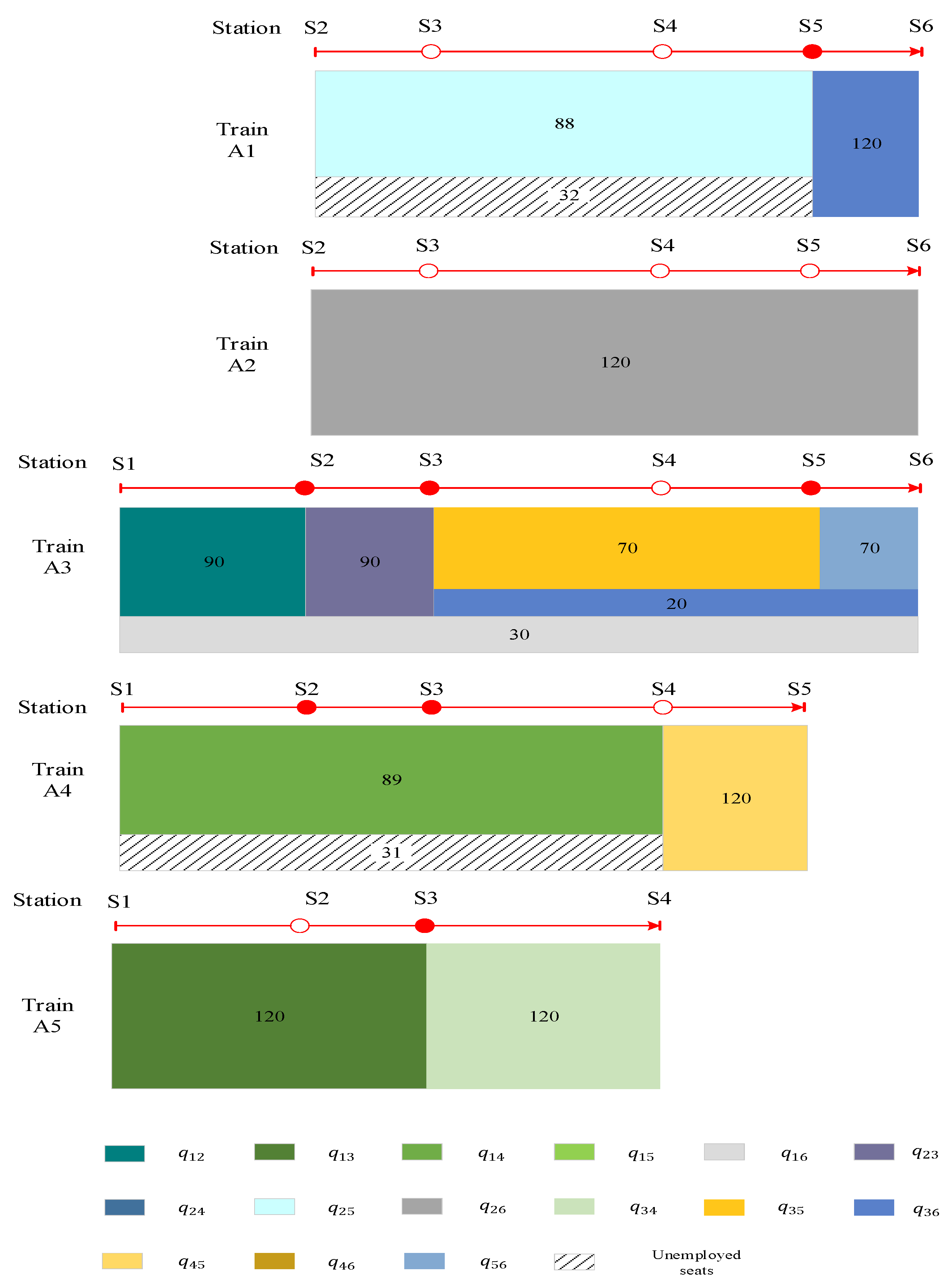
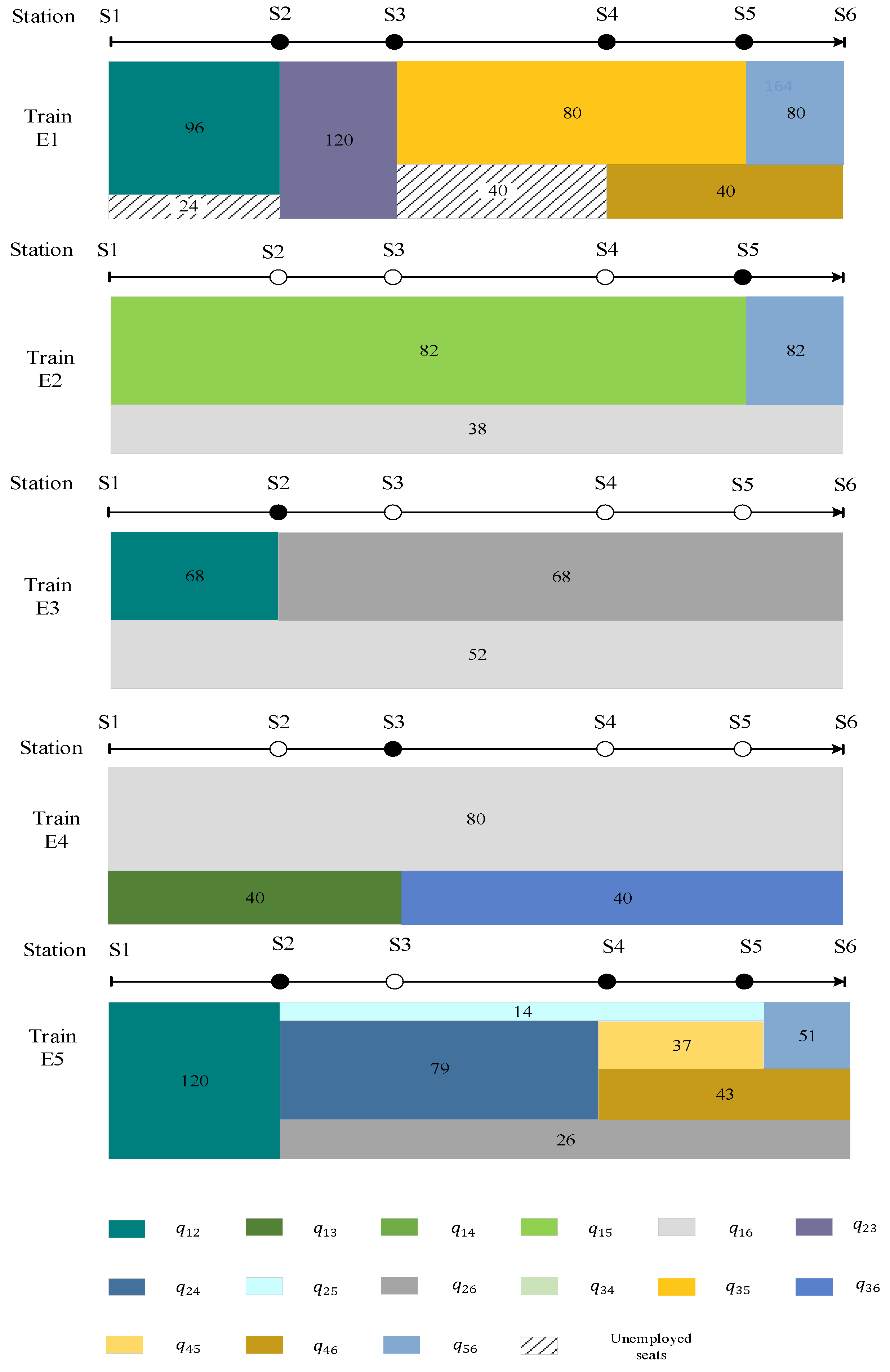
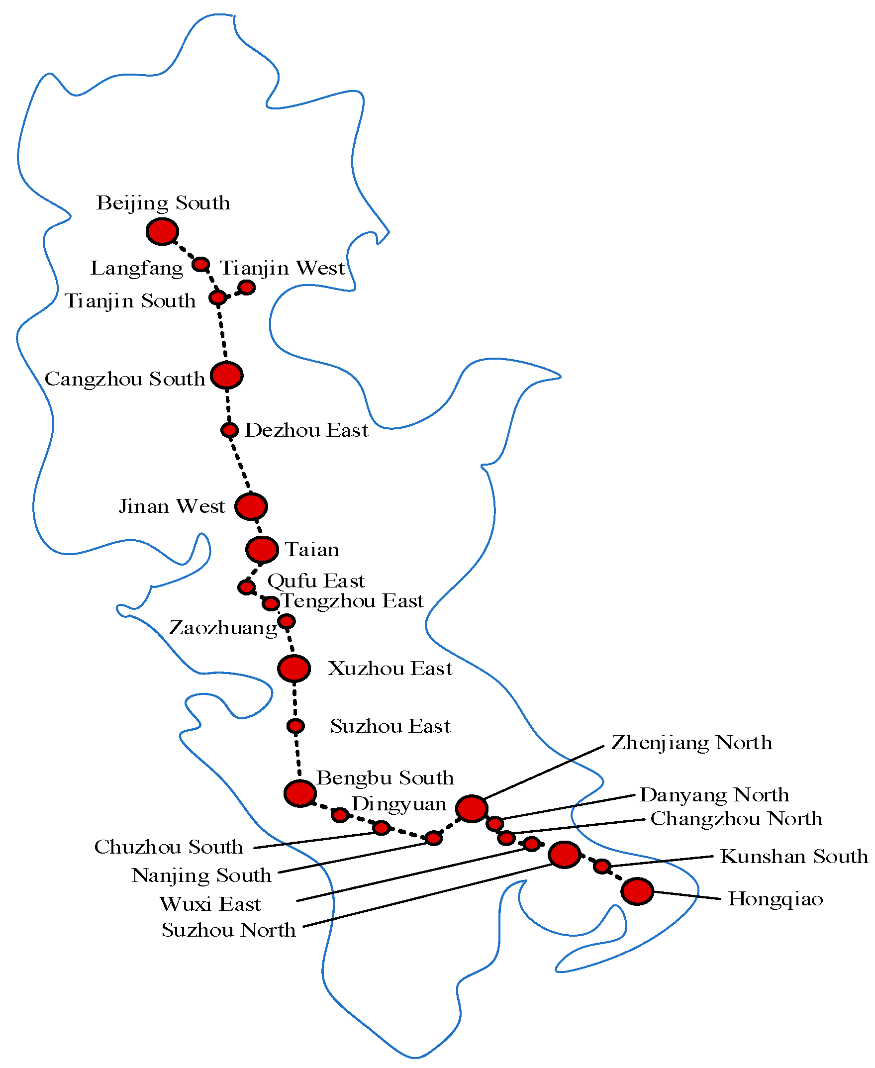
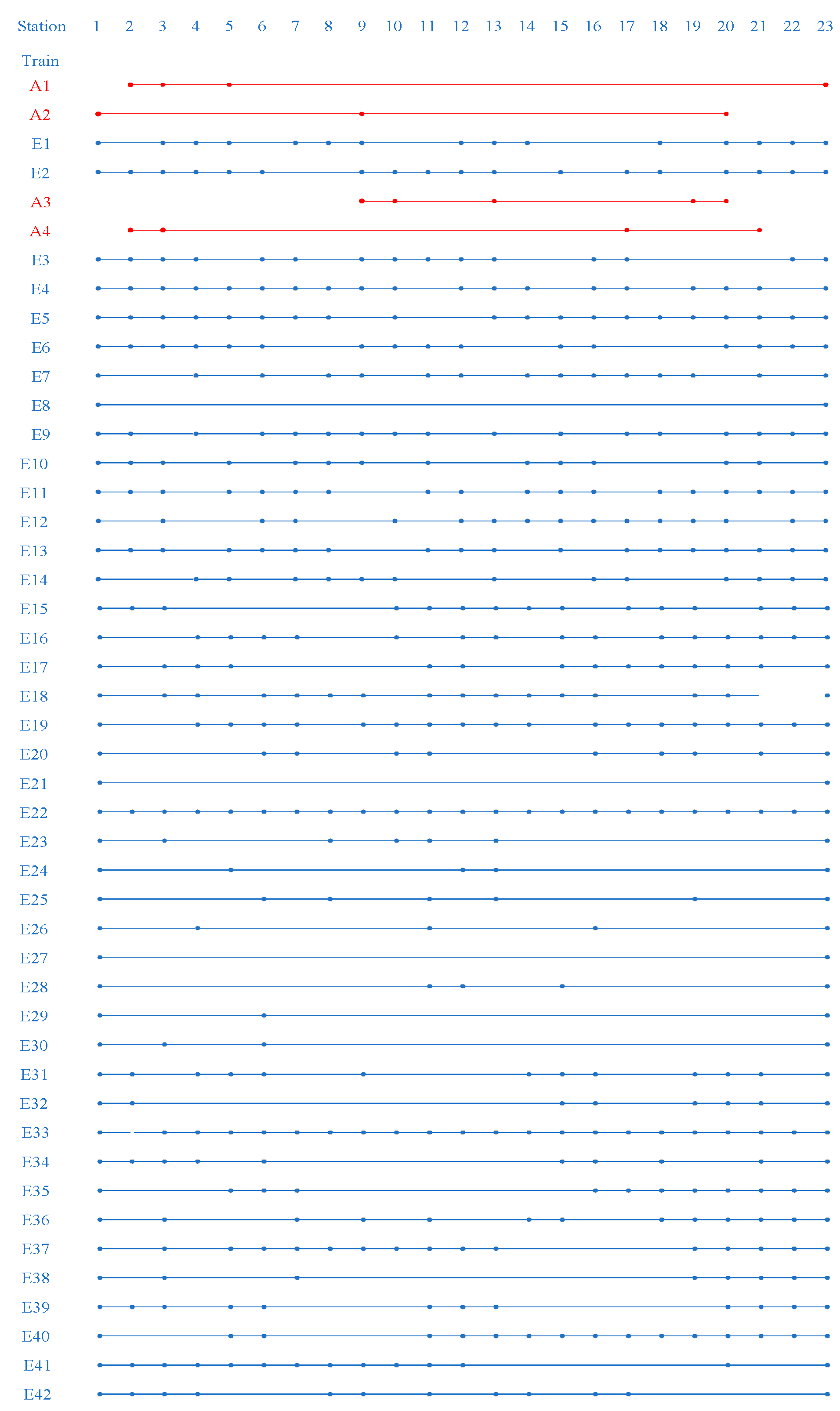
5. Numerical Experiments

In this section, several sets of experiments are implemented to test the effectiveness of our proposed model. A small-scale experiment is implemented. Furthermore, we implemented some other experiments based on the real-word data for the Wuhan‒Guangzhou railway corridor. As we know, the proposed model is an NP-hard problem. The proposed model is an integer programming model, wherein two types of decision variables, i.e., binary variables and integer variables, and constraints are reformulated into the linear type. CPLEX solver is used to solve the model. All experiments were implemented on a Windows 7 workstation with Intel Core i7 4790K CPU and 8 G RAM (Microsoft, Seattle, WA, USA, 1975).

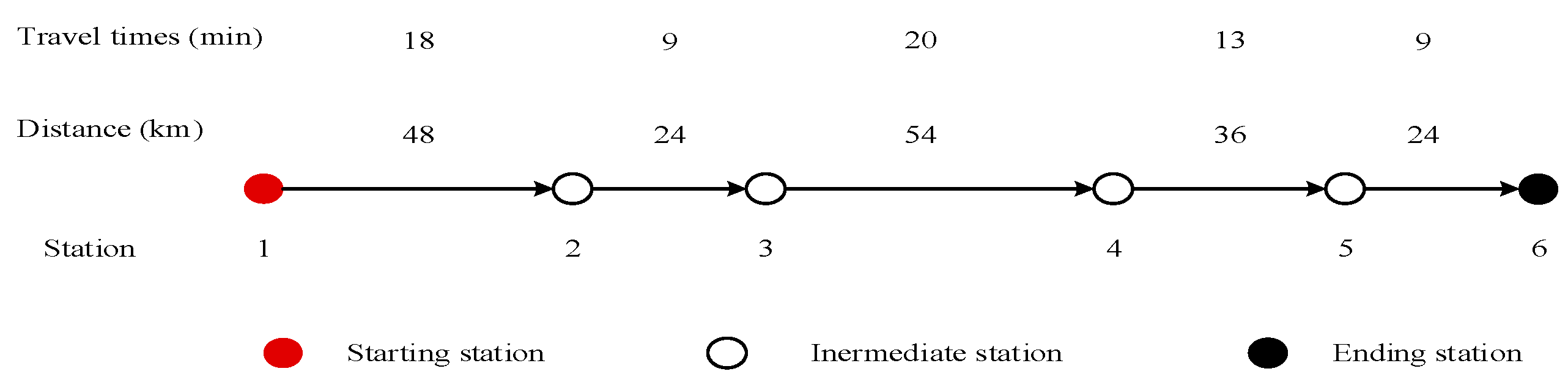
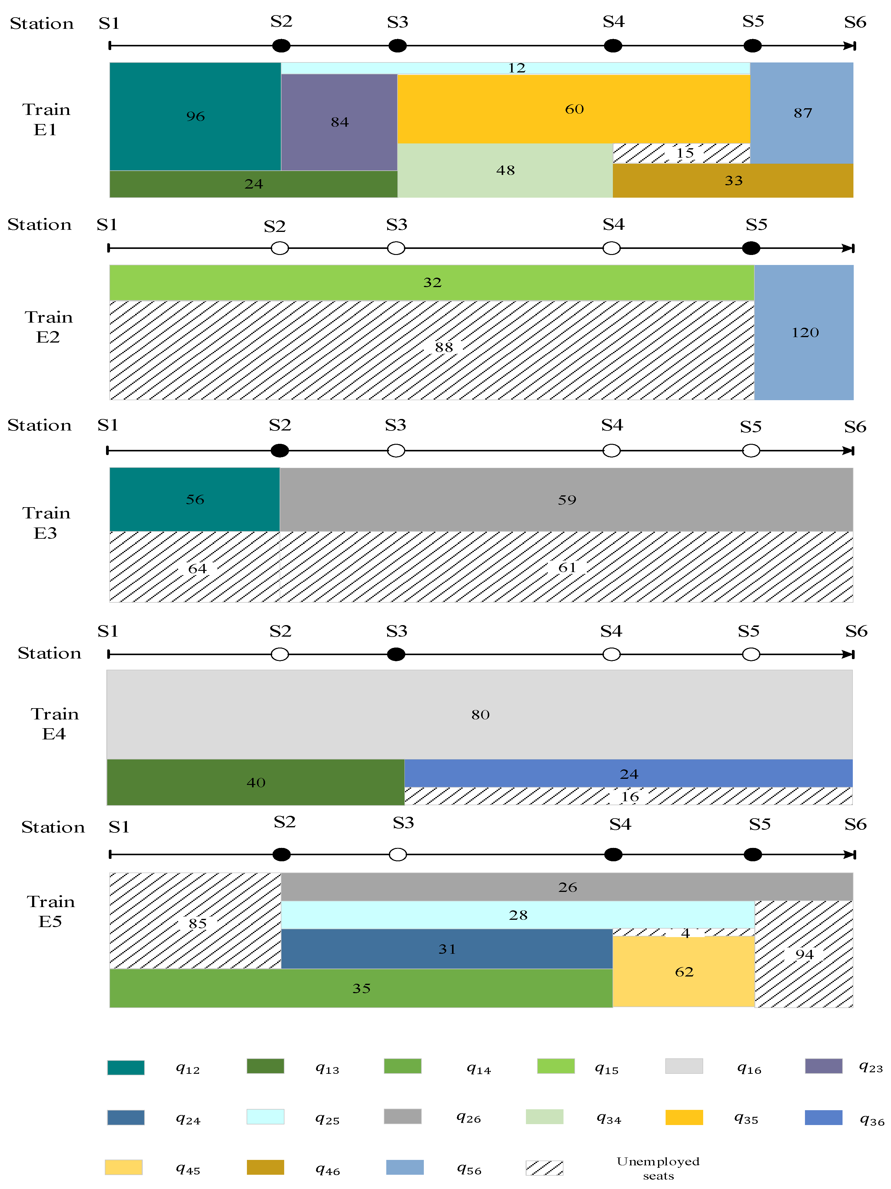
5.1. Small-Scale Case Study

The small-scale experiment is implemented on an outbound railway corridor within the time horizon $\left[0, 90\right]$ min. The railway corridor consists of six stations and five segments, as shown in Figure 3, wherein stations are indexed from the starting station of railway corridor station 1 to ending station 6 along the outbound direction. The length of each segment and travel time of trains across each segment are also displayed in Figure 3. There are five existing trains in the off-peak period. The stop plans and operational zones of these existing trains are illustrated in Figure 4. The passenger distribution plans of these existing trains are listed in Figure 4. Each train has different colored rectangles because of the different passenger distribution of each train. The length of the whole rectangle represents the maximum capacity of each train, and the width represents the total running distance of train. In Figure 4, the different colored rectangles represent passengers for different OD. The length of each colored rectangle represents the number of passengers for this OD pair. The width of each color rectangle represents the distance of the OD pair. To clarify the number of passengers for each OD in each train, the number in each rectangle denotes the number of passengers that the train takes for this OD pair. The number of empty seats in each train is also noted in these figures of passenger distribution. The passenger demand for each OD of the railway corridor in peak periods is given in

Table 6. Passenger demand for each OD in peak period.

Origin\Terminal Station	S1	S2	S3	S4	S5	S6	Total
S1	-	380	160	89	82	200	911
S2	-	-	210	79	102	214	605
S3	-	-	-	120	150	60	330
S4	-	-	-	-	157	83	240
S5	-	-	-	-	-	521	411
Total	-	380	370	288	491	1078	2607

. Obviously, transport capacity provided by the existing trains cannot meet the passenger demand. To meet passenger demand in peak periods, we intend to add five additional trains according to Equation (1). The additional trains must maintain the departure headway to avoid collisions. The minimum departure headway $h_{min}^d$ is set to 2 min. The maximum loading capacity of each train is 120. To leave enough time for passengers to board, we set the minimum dwelling time $d_{min}$ to 1 min. The capacity‒occupancy ratio is set to 0.8 to make full use of the transport capacity. Since our operational plan is meant to be passenger-responsive, the third objective of passenger demand has the highest priority in our experiments. The second objective of dwelling time has the second priority and the importance of the first objective is the lowest. Thus, the weight parameters of the three objectives ${\delta }_1$, ${\delta }_2$, and ${\delta }_3$ are set to 0.1, 0.2, and 0.7. To normalize the three objectives, we first implement two experiments maximizing and minimizing the first objective and get the values of $F_{1min}$ and $F_{1max}$, i.e., 0 and 714. Similarly, the value of $F_{2min}$ and $F_{2max}$ are 0 and 166, and $F_{3min}$ and $F_{3max}$ are 408 and 186,930.

Based on the above parameters, the optimal solution of the model is obtained. The value of the first objective function of trains’ running distance is 750 km. The value of the second objective function of dwelling time is 12 min. The value of the third function is 408 unit.km. Although we set a high weight for the third objective, 17 passengers cannot travel from origin (station 5) to destination (station 6) on train. To better illustrate the experimental results, the operational zones, stop plans, timetables, and passenger distribution for additional trains are shown in Figure 5, Figure 6 and Figure 7. Figure 5 illustrates the operational zone and stop plan for the additional trains and existing trains. The red one represents an additional train, and the black one is an existing train. S1 is station 1, E1 is the first existing train to arrive at its terminal station, and A1 is the first additional train to arrive at its terminal station. In Figure 5, a solid dot denotes a train that needs to stop at this station, and a hollow dot denotes a train that goes through this station without stopping. Figure 6 shows the timetables of additional trains and existing trains. Similarly, the red line represents the timetable of the additional train, and the black line represents the timetable of the existing train. In Figure 6, the existing trains are indexed from E1 to E5 depending on the arrival time, and additional trains are indexed from A1 to A5. The passenger distribution of the five additional trains is illustrated in Figure 7. Since the passenger distribution for existing trains is optimized jointly with additional trains in the model, the passenger distribution for existing trains has changed compared with the data in Figure 4. The new passenger distribution for existing trains is illustrated in Figure 7.

It is known from Figure 5 that the five additional trains have different operational zones and stop plans. There four kinds of operational zones for these additional trains. Train A3 has a long-distance operational zone from S1 to S6. To cut down on unnecessary running distance, the other trains do not need to select the starting station or ending station of the corridor as their origin station or terminal station. As a result, the operational zone of trains A1 and A2 is from S2 to S6. Although trains A1 and A2 have the same operational zone, they have different stop plans. Train A2 just serves the passengers from S2 to S6, with no stops at intermediate stations. Train A1 stops at S5 to serve passengers departing or arriving there. It is seen in Figure 6 that the additional trains can maintain the departure headway in relation to existing trains to avoid collisions. It is noted that additional train A3 is overtaken by existing trains E2 at S3 and E3 at S5. Train A3 arrives at S3 after 32 min and waits at S3 for 4 min to make way for train E2. Train E2 goes through S3 after 34 min without stopping. Train A3 departs from S3 36 min after E2 departs from S3 to maintain the departure‒arrival headway of 2 min with relation to train E2. Next, train A3 arrives at S5 after 69 min and waits there for 4 min to make way for train E3. In the end, train A3 arrives at S6 after 88 min. Therefore, our proposed model has the ability to choose an overtaking strategy to insert more additional trains between the existing trains and maintain the necessary headway. We know from the timetables of trains in Figure 6 that a decision maker must select suitable times and stations to insert the additional trains to maintain headway and meet passenger demand as much as possible. Timetabling decisions affect the operational zones and stop plans of additional trains and further affect passenger distribution. Thus, considering the timetables of additional trains in the operational plan is essential.

Figure 7 shows the passenger distribution of these additional trains. In the optimal operational plan, only 17 passengers cannot board trains to reach their destinations, and the trip of these unsatisfied passengers includes just one segment, i.e., S5‒S6. This verifies that long-distance passengers have the higher priority in the model. In order to keep the high use ratio of transport capacity, the capacity‒occupancy ratio of each train is over 0.8, in line with our expectations. The area of rectangles of empty seats of additional trains A2, A3, and A5 is 0. The area of rectangles of empty seats of additional trains A1 and A4 is very small. This shows that few seats are empty on each additional train. It is interesting to observe that when the capacity of each train is reached and no passengers need to alight, the train goes through and does not stop at this station. The impact of passenger distribution on the stop plan is very significant. Figure 8 shows the passenger distribution for existing trains after optimization. Although the stop plans and timetables are fixed for existing trains, the passenger distribution for existing trains is optimized in the experiment. Comparing Figure 8 with Figure 4, we find that the number of empty seats of these existing trains decreases obviously after the optimization. That shows that the model makes full use of the transport capacity of both additional trains and existing trains.

5.2. Additional Experiments

The influences of the three parameters of our proposed model, i.e., the capacity‒occupancy ratio of each train $\delta$, the minimum headway $h_{min}$, and the minimum dwelling time $d_{min}$, on the optimal solution are analyzed.

(i) Capacity–occupancy ratio

In the model, we introduce a coefficient of the capacity‒occupancy ratio, $\delta$, to control the capacity‒occupancy ratio. This coefficient is used to restrict the number of passengers along each segment belonging to the train’s operational zone. Although a higher capacity‒occupancy ratio for a single train is better, the impact of different capacity‒occupancy ratios on the final operational plan is not known. Thus, we implement several experiments using capacity‒occupancy ratio from 0.5 to 1.0 and obtain the corresponding operational plan. The experimental environment and other parameters are the same as in the small-scale case study. For computational accuracy, the relative MIP gap tolerance is set to 0.01 for the set of experiments. The detailed computational results are listed in

Table 7. Optimized solutions obtained under different capacity-occupancy ratio $\delta$.

$\mathit{\delta }$	The Number of Trains	Running Distance	Dwelling Time	The Number of Stops	Unsatisfied Passengers
0.5	5	750	10	4	17
0.6	5	750	11	5	17
0.7	5	750	11	5	17
0.8	5	750	12	6	17
0.9	4	600	5	5	208
1.0	4	576	5	5	207

.

In Table 7, some indexes of additional trains, i.e., the number of trains, the total running distance of trains, the total dwelling time, the number of stops, and unsatisfied passengers, are displayed to evaluate the operational plan. Clearly, when $\delta$ is from 0.5 to 0.8, although the stop plan is changed slightly depending on the capacity‒occupancy ratio, the number of additional trains, number of unsatisfied passengers, and running distance are the same. The reason is that the objective function of passenger demand plays a role in ensuring the capacity‒occupancy ratio to some extent. The third objective function can keep the capacity‒occupancy ratio high. When $\delta$ increases to 0.9 and 1.0, the number of additional trains decreases, and the number of unsatisfied passengers increases significantly. In the operational plan of 0.9 and 1.0, only four trains are added and the corresponding total running distance is decreased, which means lower costs for the railway company. However, the expectation of decision maker is not only for a lower cost, but also meeting more passenger demand. The number of unsatisfied passengers increases significantly, which is contrary to our aim. Generally, a high capacity‒occupancy ratio means fewer trains loading more passengers. However, in terms of designing the operational plan for multiple trains, a higher ratio is not necessarily better. Despite the number of passengers on some trains being large in the operational plan, the remaining passengers are not enough to guarantee at-capacity occupancy for other trains and so they are canceled. Thus, choosing a suitable $\delta$ value that is good for cost and passenger demand is important.

(ii) The minimum dwelling time$d_{min}$

The parameter of the minimum dwelling time $d_{min}$ is proposed to offer time for passengers to get on/off. Passengers need more dwelling time to board and alight, while the passengers staying on the train hope for less dwelling time. Next, we will test the optimal solutions under the value of $d_{min}$ from 1 to 6 min. Some meaningful indexes of optimal solutions are displayed in

Table 8. Optimized solutions obtained under the minimum dwelling time $d_{min}$.

${\mathit{d}}_{\mathit{m}\mathit{i}\mathit{n}}$	The Number of Trains	Running Distance	Dwelling Time	The Number of Stops	Unsatisfied Passengers
1	5	750	12	6	17
2	5	750	17	4	31
3	5	690	22	3	141
4	5	690	22	2	154
5	5	690	25	2	154

.

When the minimum dwelling time changes from 1 to 5, the number of trains is still five, but the running distance is decreased. With $d_{min}$ increasing, the dwelling time also increases, and the number of stops decreases. To insert more additional trains into the original operational plan and avoid conflicts with existing trains, the number of stops need to be reduced. Also, the operational zones of trains are shortened. As a result, the number of unsatisfied passengers increases, with the value of $d_{min}$ also increasing. The worst result is when the number of trains is three and $d_{min}$ is 6: the number of unsatisfied passengers rises to 400. Thus, a suitable dwelling time at a station where there are passengers getting on/off is indispensable. However, more dwelling time is not always better.

(iii) The headway $h_{min}$

In the real world, railway company operators always set a certain headway, which is not only to avoid conflicts between trains, but also to leave enough time for operators and workers to prepare. The influence of headway on the operational plan needs to be investigated. The experimental results with different values of $h_{min}$ are listed in

Table 9. Optimized solutions obtained under the minimum headway $h_{min}$.

${\mathit{h}}_{\mathit{m}\mathit{i}\mathit{n}}$	The Number of Trains	Running Distance	Dwelling Time	The Number of Stops	Unsatisfied Passengers
1	5	750	9	6	17
2	5	750	12	6	17
3	5	654	7	5	139
4	4	468	6	4	259
5	4	468	5	3	261

.

When the headway is from 1 min to 2 min, there seems to be no difference between the two operational plans. However, when we look a little more carefully at the results, the total dwelling time changes from 9 min to 12 min. The reason is that one of the additional trains dwells at one station for 4 min to give way to the existing train. That is to say that when the headway become longer, some operations, e.g., overtaking, will be performed to insert more additional trains and load more passengers. The situation is more obvious as the headway increases. When the headway increases to 6 min, all five trains cannot be inserted within the limited time horizon, and one additional train is cancelled. Meanwhile, the number of unsatisfied passengers rises to 261. It is known from this set of experiments that suitable headway can leave enough time for operators to prepare and avoid collisions. Therefore, the value of the headway should be selected carefully in real-world operations.

(iv) The minimum number of boarding and alighting persons for stopping, $y_{min}$

$y_{min}$ is the minimum number of boarding and alighting persons required for a train to stop. Stopping consumes energy to accelerate and decelerate, which increases the railway company’s costs. Therefore, operators are very serious about designing a stop plan. The required minimum number of persons boarding and alighting for stopping is proposed in the model, which means that the train cannot stop at a station until the sum of boarding and alighting persons is up to a certain threshold. We select 10 different values of $y_{min}$, from 10 to 100, and the corresponding solutions are listed in

Table 10. Optimized solutions obtained under the minimum dwelling time $y_{min}$.

${\mathit{y}}_{\mathit{m}\mathit{i}\mathit{n}}$	The Number of Trains	Running Distance	Dwelling Time	The Number of Stops	Unsatisfied Passengers
10	5	750	12	6	17
20	5	750	12	6	17
30	5	750	12	6	17
40	5	750	11	5	32
50	5	750	11	5	32
60	5	690	5	4	142
70	5	690	5	4	142
80	5	690	5	4	142
90	4	600	4	3	210
100	4	576	3	2	252

. From Table 10, the number of trains, running distance, dwelling time, and number of stops tends to decrease, while the number of unsatisfied passengers tends to increase. On the face of it, increasing the threshold for stopping can decrease the dwelling time, the number of stops, and the number of trains, which can reduce costs. However, more passengers may not be able to board the trains. Hence, in the real world, selecting the threshold for stopping is important for operators. In addition, more passenger demand is met, which can bring about benefits for the railway company. There is a need to consider the relationship between energy consumption and the price of a ticket, which will be considered in further research.

5.3. Large-Scale Case Study

In this section, we will test the performance by applying the proposed model to designing an operational plan for high-speed trains on the Beijing‒Shanghai high-speed railway corridor in China. The Beijing‒Shanghai railway corridor is the main railway corridor connecting Beijing and Shanghai and one of the country’s most important corridors. The experimental data in this large-scale study are real-world data.

Before implementing the large-scale experiment, we first introduce the input experimental data. We implement this experiment within [0, 720] min on the Beijing‒Shanghai corridor. As shown in Figure 9, the Beijing‒Shanghai railway corridor has a total length of 1318 km and consists of 24 stations and 23 segments [29]. The details on the distance of each segment and the traveling time of high-speed trains in each segment are listed in

Table 11. Distance and traveling time.

Segment	Distance (km)	Traveling Time (min)
Beijing South-Langfang	59	21
Langfang-Tianjin	72	18
Tianjin South-Cangzhou West	88	22
Cangzhou West-Dezhou East	108	27
Dezhou East-Jinan West	92	24
Jinan West-Taian	43	18
Taian-Qufu East	71	22
Qufu East-Tengzhou	56	17
Tengzhou-Zhaozhuang	36	13
Zhaozhuang-Xuzhou East	63	18
Xuzhou East-Suzhou East	79	19
Suzhou East-Bengbu South	77	23
Bengbu South-Dingyuan	53	16
Dingyuan-Chuzhou	62	19
Chuzhou-Nanjing South	59	18
Nanjing South-Zhenjiang South	69	20
Zhenjiang South-Danyang North	25	11
Danyang North-Changzhou North	32	11
Changzhou North-Wuxi East	57	17
Wuxi East-Suzhou North	26	10
Suzhou North-Kunshan South	32	11
Kunshan South-Hongqiao	43	18

[30].

There are 24 stations along the Beijing‒Shanghai railway corridor. Since Tianjin South Station and Tianjin North Station both belong to the city of Tianjin, we do not consider the difference in passenger demand between the two stations; their passenger demand is combined and regarded as the passenger demand at Tianjin Station. Thus, there are totally 23 × 22/2 = 253 OD pairs. The OD passenger demand associated with stations on the Beijing‒Shanghai railway corridor in peak periods is listed in

Table 12. (a) Passenger demand for each OD pair. (b) Passenger demand for each OD pair.

Origin/Terminal Station	Beijing South	Langfang	Tianjin	Cangzhou West	Dezhou East	Jinan West	Taian	Qufu East	Tengzhou	Zhaozhuang	Xuzhou East	Suzhou East
Beijing South	_	701	4427	1863	1490	3901	1512	2016	273	438	2696	460
Langfang	_	_	832	548	350	350	98	100	69	104	121	100
Tianjin	_	_	_	1315	1424	2301	613	1424	176	328	2235	240
Cangzhou West	_	_	_	_	219	394	88	88	10	44	196	21
Dezhou East	_	_	_	_	_	832	284	352	44	219	219	112
Jinan West	_	_	_	_	_	_	1183	1140	56	1227	1030	73
Taian	_	_	_	_	_	_	_	284	42	307	723	108
Qufu East	_	_	_	_	_	_	_	_	28	175	219	438
Tengzhou	_	_	_	_	_	_	_	_	_	52	125	53
Zhaozhuang	_	_	_	_	_	_	_	_	_	_	394	284
Xuzhou East	_	_	_	_	_	_	_	_	_	_	_	416
Suzhou East	_	_	_	_	_	_	_	_	_	_	_	_
(a)
Origin/Desitination	Bengbu South	Dingyuan	Chuzhou	Nanjing South	Zhenjiang South	Danyang North	Changzhou North	Wuxi East	Suzhou North	Kunshan South	Hongqiao
Beijing South	789	249	411	328	416	236	657	592	525	416	1302
Langfang	113	44	175	416	101	62	108	107	102	100	1243
Tianjin South	1052	171	219	1336	284	160	306	328	240	210	1171
Cangzhou West	109	12	21	394	65	14	112	112	87	65	1083
Dezhou East	175	57	105	394	109	53	131	132	112	112	975
Jinan West	263	54	108	1644	306	60	438	438	372	328	883
Taian	109	49	42	548	87	45	175	176	153	131	840
Qufu East	87	33	21	613	131	31	175	175	173	153	769
Tengzhou	52	10	54	81	43	12	36	29	52	27	713
Zhaozhuang	285	59	219	262	97	54	196	197	196	197	677
Xuzhou East	854	187	701	1928	548	170	657	854	832	657	614
Suzhou East	_	96	832	767	284	107	306	307	175	263	535
Bengbu South	_	_	701	898	657	91	723	767	788	701	458
Dingyuan	_	_	_	71	28	12	27	33	32	36	405
Chuzhou	_	_	_	_	175	113	219	525	592	548	343
Nanjing South	_	_	_	_	526	203	592	636	1073	569	284
Zhenjiang South	_	_	_	_	_	21	788	24	679	24	215
Danyang North	_	_	_	_	_	_	24	32	34	21	190
Changzhou North	_	_	_	_	_	_	_	482	1928	482	158
Wuxi East	_	_	_	_	_	_	_	_	2892	1008	101
Suzhou North	_	_	_	_	_	_	_	_	_	1205	75
Kunshan South	_	_	_	_	_	_	_	_	_	_	43
Hongqiao	_	_	_	_	_	_	_	_	_	_	_
(b)

a,b [30]. In this experiment, we designate 42 existing trains for the off-peak period. The timetables of these 42 existing trains are illustrated in Figure 10, where the black lines represent the timetables of existing trains. The stop plans for existing trains are also illustrated in Figure 11. The rolling stock used on the Beijing–Shanghai high-speed railway corridor is usually CR400AF. There are three marshalling types of CR400AF: eight marshalling types, 16 marshalling types, and 17 marshalling types, and their capacity are 576, 1193, and 1283. In the peak period, rolling stock with large capacity is employed. Thus, the maximum loading capacity of trains is set to 1200 unit in this paper. The total passenger demand along the Beijing‒Shanghai corridor is 132,358. The total passenger demand distributed for existing trains is 112,601. There are still 19,757 passengers who cannot travel by train in the peak period. Based on the passenger demand in the peak period and the number of existing trains, we intend to add four trains. The minimum departure headway $h_{min}^d$ is set to 2 min. The minimum dwelling time $d_{min}$ is set to 2 min. To avoid wasting the transport capacity, the capacity‒occupancy ratio for both existing trains and additional trains is set to 0.7. In our paper, because the purpose of adding additional trains is to meet passenger demand in peak periods, the objective of passenger demand has the highest priority in this experiment. The weight of the third objective ${\delta }_3$ is set to 0.7. However, the cost to the railway company and the service for in-train passengers cannot be ignored. The weight parameters of the first objective about running distance ${\delta }_1$ and the second objective about dwelling time ${\delta }_2$ are set to 0.1 and 0.2. To normalize the three objectives, we implement three experiments for maximizing $F_1$,$F_2$, and $F_3$ and get the values of $F_{1max}$, $F_{2max}$, and $F_{3max}$: 10,416, 720, and 9,882,700. Similarly, we find that the values of $F_{1min}$, $F_{2min}$, and $F_{3min}$ are 0 by implementing experiments for minimizing $F_1$,$F_2$, and $F_3$.

Based on the data above, we implemented a large-scale experiment and obtained a new operational plan for peak periods. In the new operational plan, although the timetables and stop plans for existing trains were unchanged, the passenger distribution for existing trains was optimized to meet passenger demand in peak periods. The capacity‒occupancy ratio of existing off-peak trains is 0.79, which rises to 0.8 after optimization. This means that the model can improve the capacity‒occupancy ratio for existing trains to meet passenger demand in peak periods. Here, 19,757 passengers’ travel demand was not satisfied, and four additional trains were added. Four additional trains provide significant transport capacity, so just 23 passengers’ travel demand remained unsatisfied. These 23 passengers can travel by transferring or using other modes of transportation, which means the model can meet most of the passenger demand. The timetables for these four additional trains are given in Figure 10. As shown in Figure 10, two additional trains have overtaking ability at Tengzhou East and Dingyuan stations, etc. Meanwhile, all trains can maintain headway in relation to both existing trains. Stop plans for additional trains in peak periods are given in Figure 11. In Figure 11, stations are labeled 1 to 23 in the order Beijing South, Langfang, Tianjin, Cangzhou West, Dezhou East, Taian, Qufu East, Zhaozhuang, Xuzhou East, Suzhou East, Bengbu South, Dingyuan, Chuzhou, Nanjing South, Zhenjiang South, Danyang North, Changzhou North, Wuxi East, Suzhou North, Kunshan South, and Hongqiao. The dots represent trains that stop at these stations, and lines represent trains that go through these stations. It is seen from Figure 11 that these four additional trains have different operational zones. There are additional long-distance trains, e.g., train A1 from Langfang to Hongqiao. There is also an additional short-distance train, e.g., train A3 from Tengzhou East to Wuxi East.

6. Conclusions

The problem of designing an operational plan for additional trains to meet the passenger demand in peak periods is studied in this paper. We present an optimization approach for designing the operational plan for additional trains, which saved time. In this approach, all plans, including operational zones, the number of trains, stop plans, timetables, and passenger distribution, can be optimized simultaneously. A multi-objective nonlinear programming model was proposed to formulate this approach. Three objective functions are presented in the model. The goal of this paper was meeting more passenger demand in peak periods. Minimizing the deviation between the passenger demand and the transport capacity was the primary objective. Meanwhile, operating costs and passenger service on trains cannot be ignored. Minimizing the dwelling time and running distance of trains were the other two objectives. In the model, some constraints are introduced to formulate the railway system operations. OD passenger demand is specifically considered, and the constraints of passenger demand are distributed between the train. The big-$M$ is introduced to reformulate the nonlinear model into a linear model. Two series of experiments are implemented to show the performance of the proposed approach. A small-scale experiment is conducted to demonstrate that the approach can be used to obtain a good operational plan for additional trains. Furthermore, a series of small-scale experiments are conducted to analyze the effect of the parameters on the results. A large-scale experiment based on the Beijing‒Shanghai railway corridor is conducted to illustrate the application of the proposed approach to large-scale and real-word situations. This paper provides an optimization approach for railway companies to schedule additional trains in peak periods. Railways should use a scientific optimization method to design an operational plan for additional trains instead of relying on experience. The studied method can obtain good results on the railway corridor.

The passenger demand for trains in the real word is dynamic and stochastic. Considering the dynamic and stochastic nature of the model will allow us to obtain a more reasonable and practical operational plan. Moreover, adding additional trains at passengers’ preferred boarding times can provide more convenience. Passengers’ boarding time preference will be considered in future work.

References

1. The 2018 Statistical Communique on the Development of the Transport Industry. Available online: http://xxgk.mot.gov.cn/jigou/zhghs/201904/t20190412_3186720.html (accessed on 12 October 2019).
2. Burdett, R.L.; Kozan, E. Techniques for inserting additional trains into existing timetables. Transp. Res. Part B 2009, 43, 821–836. [Google Scholar] [CrossRef] [Green Version]
3. Cacchiani, V.; Caprara, A.; Toth, P. Scheduling extra freight trains on railway networks. Transp. Res. Part B 2010, 44, 215–231. [Google Scholar] [CrossRef]
4. Gao, Y.; Kroon, L.; Yang, L.; Gao, Z. Three-stage optimization method for the problem of scheduling additional trains on a high-speed rail corridor. Omega 2017, 30, 175–191. [Google Scholar] [CrossRef]
5. Liu, Y.; Cao, C.; Feng, Z.; Zhou, Y. A Cost and Passenger Responsible Optimization Method for the Operation Plan of Additional High-Speed Trains in a Peak Period. J. Adv. Transp. 2020, 2020, 3602727. [Google Scholar] [CrossRef] [Green Version]
6. Caprara, A.; Kroon, L.G.; Monaci, M.; Peeters, M.; Toth, P. Passenger Railway Optimization. In Handbooks in Operations Research and Management Science; Elsevier: Amsterdam, The Netherlands, 2007; Volume 14, pp. 129–187. [Google Scholar]
7. Bussieck, M.R.; Kreuzer, P.; Zimmermann, U.T. Optimal lines for railway systems. Eur. J. Oper. Res. 1996, 96, 54–63. [Google Scholar] [CrossRef]
8. Claessens, M.T.; van Dijk, N.M.; Zwaneveld, P.J. Cost optimal allocation of passenger lines. Eur. J. Oper. Res. 1998, 110, 474–489. [Google Scholar] [CrossRef]
9. Chang, Y.H.; Yeh, C.H.; Shen, C.C. A multi-objective model for passenger train services planning application to Taiwan’s high-speed rail line. Transp. Res. Part B 2000, 34, 91–106. [Google Scholar] [CrossRef]
10. Goossens, J.W.; Hoesel, S.V.; Kroon, L. A branch-cut approach for solving railway line-planning problems. Transp. Sci. 2004, 38, 379–393. [Google Scholar] [CrossRef] [Green Version]
11. Goossens, J.W.; Hoesel, S.V.; Kroon, L. On solving multi-type railway line planning problems. Eur. J. Oper. Res. 2005, 168, 403–424. [Google Scholar] [CrossRef]
12. Scholl, S. Customer-Oriented Line Planning. Ph.D. Thesis, Universitaet at Goettingen, Goettingen, Germany, 2005. [Google Scholar]
13. Szpigel, B. Optimal train scheduling on a single-track railway. Oper. Res. 1973, 72, 343–352. [Google Scholar]
14. Caprara, A.; Fischetti, M.; Toth, P. Modeling and solving the train timetabling problem. Oper. Res. 2002, 50, 851–861. [Google Scholar] [CrossRef]
15. Caprara, A.; Monaci, M.; Toth, P.; Guida, P.L. A Lagrangian heuristic algorithm for a real-world train timetabling problem. Discret. Appl. Math. 2006, 154, 738–753. [Google Scholar] [CrossRef]
16. Higgins, A.; Kozan, E.; Ferreira, L. Optimal scheduling of trains on a single line track. Transp. Res. Part B 1996, 30, 147–161. [Google Scholar] [CrossRef] [Green Version]
17. Higgins, A.; Kozan, E. Modeling train delays in urban networks. Transp. Sci. 1998, 32, 346–357. [Google Scholar] [CrossRef]
18. Şahin, İ. Railway traffic control and train scheduling based on inter-train conflict management. Transp. Res. Part B 1999, 33, 511–534. [Google Scholar] [CrossRef]
19. D’Ariano, A.; Pacciarelli, D.; Pranzo, M. Assessment of flexible timetables in real-time traffic management of a railway bottleneck. Transp. Res. Part C 2008, 16, 232–245. [Google Scholar] [CrossRef]
20. Canca, D.; Barrena, E.; Algaba, E.; Zarzo, A. Design and analysis of demand-adapted railway timetables. J. Adv. Transp. 2014, 48, 119–137. [Google Scholar] [CrossRef] [Green Version]
21. Barrena, E.; Canca, D.; Coelho, L.C.; Laporte, G. Single-line rail rapid transit timetabling under dynamic passenger demand. Transp. Res. Part B 2014, 70, 134–150. [Google Scholar] [CrossRef]
22. Sun, L.; Jin, J.G.; Lee, D.H.; Axhausen, K.W.; Erath, A. Demand-driven timetable design for metro services. Transp. Res. Part C 2014, 46, 284–299. [Google Scholar] [CrossRef]
23. Zhang, T.; Li, D.; Qiao, Y. Comprehensive Optimization of Urban Rail Transit Timetable by Minimizing Total Travel Times under Time-dependent Passenger Demand and Congested Conditions. Appl. Math. Model. 2018, 58, 421–446. [Google Scholar] [CrossRef]
24. Robenek, T.; Azadeh, S.S.; Maknoon, Y.; De Lapparent, M.; Bierlaire, M. Train timetable design under elastic passenger demand. Transp. Res. Part B 2018, 111, 19–38. [Google Scholar] [CrossRef] [Green Version]
25. Fu, H.; Sperry, B.R.; Nie, L. Operational impacts of using restricted passenger flow assignment in high-speed train stop scheduling problem. Math. Probl. Eng. 2013, 78, 143–175. [Google Scholar] [CrossRef]
26. Chen, D.; Ni, S.; Xu, C.A.; Lv, H.; Wang, S. High-Speed Train Stop-Schedule Optimization Based on Passenger Travel Convenience. Math. Probl. Eng. 2016, 2016, 8763589. [Google Scholar] [CrossRef] [Green Version]
27. Qi, J.; Li, S.; Gao, Y.; Yang, K.; Liu, P. Joint optimization model for train scheduling and train stop planning with passengers distribution on railway corridors. J. Oper. Res. Soc. 2018, 69, 556–570. [Google Scholar] [CrossRef]
28. Qi, J.; Yang, L.; Di, Z.; Li, S.; Yang, K.; Gao, Y. Integrated optimization for train operation zone and stop plan with passenger distributions. Transp. Res. Part E 2018, 109, 151–173. [Google Scholar] [CrossRef]
29. Yi, M. Optimization Research on Beijing-Shanghai Stop Schedule Plan of High-Speed Railway. Master’s Thesis, Southwest Jiaotong University, Chengdu, China, 2005. [Google Scholar]
30. Yang, L.; Qi, J.; Li, S.; Gao, Y. Collaborative optimization for train scheduling and train stop planning on high-speed railways. Omega 2016, 64, 57–76. [Google Scholar] [CrossRef]
Figure 1. Adding additional train on a railway corridor in the peak period.
Applsci 10 05554 g001
Figure 2. An illustration of operation zones and stop plans for additional trains.
Applsci 10 05554 g002
Figure 3. A small-scale outbound railway corridor.
Applsci 10 05554 g003
Figure 4. Passenger distribution for existing trains.
Applsci 10 05554 g004
Figure 5. Stop plans for existing trains and additional train.
Applsci 10 05554 g005
Figure 6. Timetables for existing trains and additional train.
Applsci 10 05554 g006
Figure 7. Passenger distribution for additional trains.
Applsci 10 05554 g007
Figure 8. Passenger distribution for existing trains.
Applsci 10 05554 g008
Figure 9. Map of Beijing-Shanghai high-speed railway corridor.
Applsci 10 05554 g009
Figure 10. Timetables for existing trains and additional trains on Beijing–Shanghai railway corridor.
Applsci 10 05554 g010
Figure 11. Stop plans for existing trains and additional trains on Beijing–Shanghai railway corridor.
Applsci 10 05554 g011