1. Introduction
The past few years have been decisive for the foundation of a new global era, being especially notorious the impact of a diverse set of forces and trends associated with the acceleration of scientific and technological discoveries in the field of information. The flourishing of the Information Age promotes the momentum of the Internet of Things (IoT), which entails an environment pervaded by vast amounts of intelligent devices capable of sensing, capturing, computing and operating the real world [
1]. Everyday, these devices generate continuous streams of real-time data. The magnitude of the daily explosion of data has led to the emergence of the Big Data paradigm.
There is therefore a large amount of data being produced and disseminated throughout the world on a daily basis. Although this vast amount of data may appear to be meaningful in decision-making processes, in reality, people are overwhelmed by this continuous flow of data [
2,
3]. With the evolution of technology and the exponential growth of information available, the population is starting to struggle to find what they need or prefer.
The value of data is not immediate, and it must travel a long way before it reaches its highest purpose, gaining incremental value as it goes. The data flow is characterized by a variety of steps required to transform low-value inputs, the raw data, into high-value outputs, actionable information and useful insights. Manually processing existing data is tedious, inefficient, and often leads to errors. In addition, it is difficult to classify, filter and then recommend from such a huge set of data. A more efficient approach is to automatically process user’s opinions, features, and other related data in order to predict a new set of related products. Recommendation systems have appeared as a solution to this problem and have been receiving a great deal of attention and use from the scientific community in recent years.
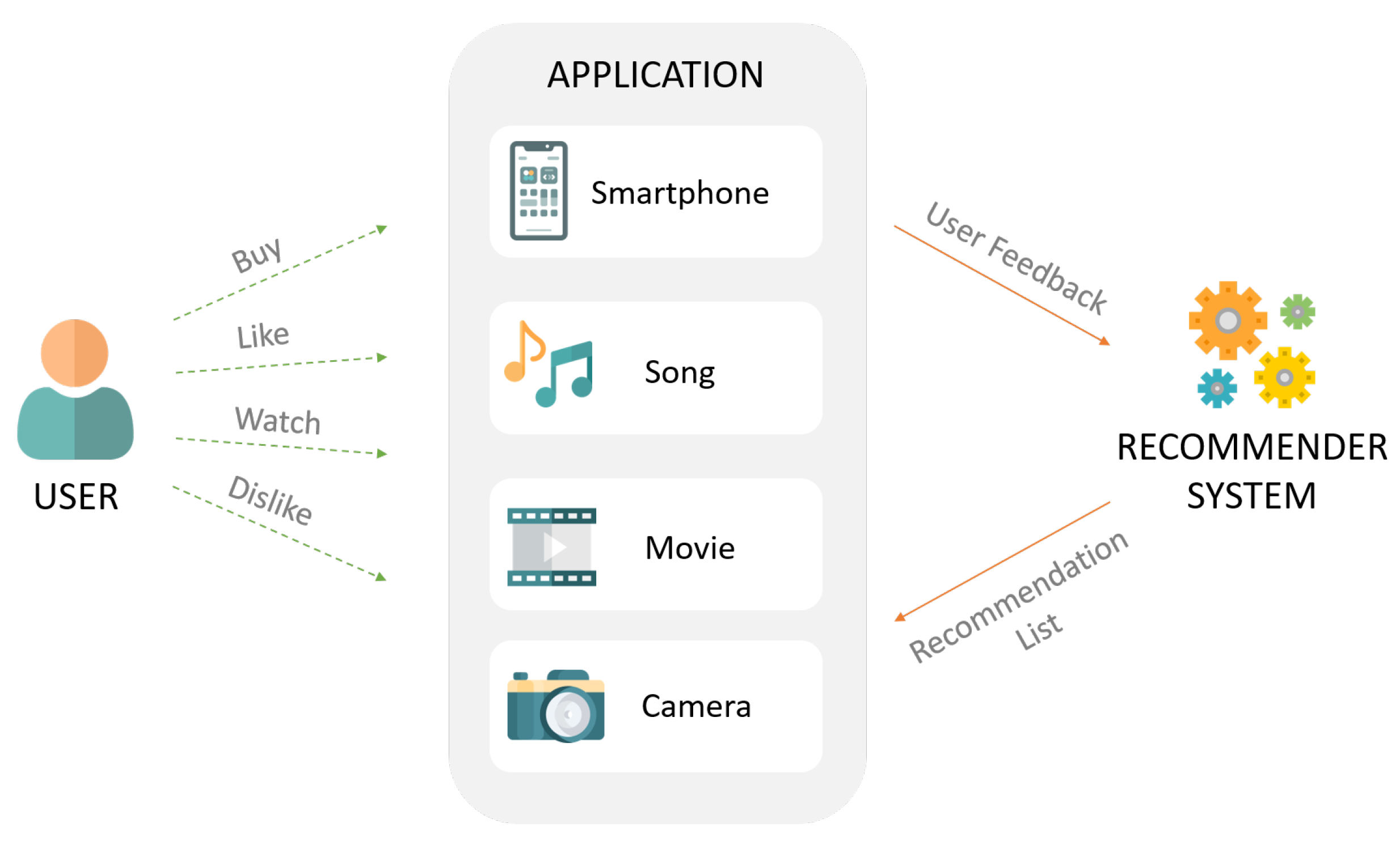
Recommender systems are information search and filtering tools that help users to discover relevant items and to make better choices while searching for products or services such as movies, books, vacations, or electronic products. The fundamental goal of a recommender system is to reduce the information overload and to provide personalized suggestions that can assist the users in the decision-making process [
4,
5].
Figure 1 shows the generic operation behind the recommendation systems in a simplified way. However, these systems usually face certain limitations and challenges due to the increasing demand of high-quality personalization and recommendation [
4,
6].
Recommendation systems have become a valuable asset regardless of the application domain. Nowadays, Internet users turn to the
WorldWideWeb for help in the planning and selection of many everyday tasks, whether it is what music to listen to (Spotify), what consumer products to purchase (Amazon, AliExpress), what movies to watch (Netflix) and so on. Furthermore, social networks such as LinkedIn, YouTube and Facebook have also included recommendation technologies to suggest groups to join, people to follow, videos to watch or posts to like [
7].
Although the origins of recommender systems can be traced back to the extensive work in cognitive science [
8], approximation theory [
9], information retrieval [
10], forecasting theories [
11], and also have bonds to management science [
12] and to consumer choice modeling in marketing [
13], recommender systems emerged as an independent research area in the mid-1990s when investigators started focusing on recommendation problems that explicitly rely on the rating structure. In its most basic formulation, the recommendation problem is reduced to the difficulty of determining ratings for items that have not been seen by the user. Generally, this estimation is based on the ratings given by the user to other items and on some other knowledge. Once it becomes possible to estimate the ratings for the items that have not yet been rated, it will be feasible to recommend the items with the highest estimated ratings to the user [
4].
Being part of intelligent systems, recommender systems use several kinds of knowledge. The knowledge needed to produce recommendations have four sources: from the user itself, from other peer users of the system, from data regarding the items being recommended, and lastly from the recommendation field itself, knowledge about how recommended items are applied and what needs they satisfy [
14].
Recommendation systems can be divided into three main categories [
4]—Content-based Recommendations, Collaborative Recommendations, and Hybrid Recommendations. In the first approach, the user will be recommended items similar to those he/she enjoyed in the past. In turn, in the collaborative approach, recommendations are made based on items consumed by users whose tastes and preferences are similar to that of the referred user. Finally, combining content-based and collaborative recommendations leads to hybrid approaches, which are regularly applied, since both types of recommendations can be complemented by one another [
15].
Human beings have always sought opinions or advice on items through conversations with friends, store staff, and even through the reading of comments on products, to help them in the decision-making process. This is the basis of Collaborative Filtering, which uses other people’s opinions to make a recommendation. Collaborative filtering techniques can be divided into two categories: memory-based (user/item-based) and model-based [
16]. Memory-based algorithms act on the entire user/item matrix. They assume that users/items can be grouped together by similarity. On the other hand, model-based techniques use a set of user assessments to generate an estimated model, saving the parameters learned during training. Instead of using similarity measurements, these algorithms are characterized by the creation of models [
17].
Matrix Factorization [
18], one of the techniques used in collaborative model-based filtering, is a well-established algorithm in the recommendation system’s literature. It is a model that achieves a decent performance in the task of predicting ratings, standing out the Principal Component Analysis (PCA) and Singular Value Decomposition (SVD) models. But it turns out to be essentially a linear model, making it impossible to capture complex nonlinear and intricate relationships that can be predictive of users’ preferences [
19].
Today, with the concept of deep learning becoming more important, several researchers have begun to test its usability in a collaborative filtering approach in order to achieve better results [
20]. For example, Van den Oord et al. made use of deep convolutional neural network to give music recommendations [
21]. Deep models can learn high-order features of input data which may be useful for recommendation as indicated in Reference [
22]. Autoencoders are a common building block of Deep Learning architectures [
20,
23].
In this article, an autoencoder is used for collaborative filtering tasks with the aim of giving product recommendations. An autoencoder is a neural network that learns to copy its input to its output in order to encode the inputs into a hidden (and usually low-dimensional) representation [
19]. Neural networks have proven to be capable of approximating any continuous function, making it suitable for addressing the limitation of matrix factorization and enhancing the expressiveness of matrix factorization [
19]. A comparison of the results will also be made between the SVD and the autoencoder using the Root Mean Square Error (RMSE) metric.
The organization of the remainder of the paper is as follows—
Section 2 will present the related work on collaborative filtering, autoencoders, and SVD. The methodology used in this study will be presented in
Section 3, where a small overview of the datasets used, the data preparation, the architecture of the autoencoder as well as some evaluation metrics will be discussed.
Section 4 will present the main findings and their discussion. Finally,
Section 5 concludes this article and points out possible future work.
2. Related Work
In the context of recommendation systems, several solutions have emerged using collaborative filtering to help users find items that meet their interests and also benefit different organizations and sectors in order to captivate their customers.
In the literature several approaches can be found to achieve goals similar to this article. As an example, R. YiBo and G. SongJie have implemented a recommendation system using an algorithm based on SVD smoothing that predicts item ratings that users have not yet rated by employing SVD technology, and then uses Pearson’s similarity correlation measurement to find neighbors for the target users, and finally makes recommendations [
24]. S. Badrul et al. propose and experimentally validate a technique that has the potential to incrementally build SVD-based models and promises to make the recommender systems highly scalable [
25]. B. Qilong et al. propose a new approach combining a clustering algorithm with an SVD algorithm that is widely used in the domain of image-processing into a collaborative filtering algorithm. Then they decompose the rating matrix with the SVD algorithm and merge them into a new rating matrix to calculate the similarity between each pair of users. At last, they take advantage of the similarity to find the nearest neighbors in the collaborative filtering recommendation and predict the ratings of the items to make the recommendation [
26].
However, most recommendation systems still face challenges in dealing with the enormous volume, complexity and dynamics of data [
27]. In order to address these issues, a number of researchers have dedicated themselves to improving recommendation systems by integrating deep learning techniques. The first attempts to use deep learning for recommendation systems began with the use of restricted Boltzman machines (RBMs) [
22]. However, several recent approaches have been using autoencoders. For example, H. T. Dai et al. built a flexible Deep Autoencoder (DAE) model, named FlexEncoder, that uses configurable parameters and unique features to analyze the parameter influence on the prediction accuracy of recommender systems [
28]. S. Suvash et al. propose AutoRec, a novel autoencoder framework for collaborative filtering (CF). Empirically, AutoRec’s compact and efficiently trainable model outperforms state-of-the-art CF techniques (biased matrix factorization, RBM-CF and LLORMA) on the Movielens and Netflix datasets [
29]. C. Sanxing et al. propose a novel CF method that uses a stacked auto-encoder with denoising, an unsupervised deep learning method, to extract the useful low-dimensional features from the original sparse user-item matrices [
30]. O. Yuanxin et al. proposed an autoencoder based on collaborative filtering method, which provides pre-training and stacking mechanisms. The experimental study on commonly used MovieLens datasets have shown its potential and efficacy in achieving higher recall [
31]. Another work developed, where autoencoders were used, was that of Li, X., & She, J [
32] who proposed a Bayesian generative model called collaborative variational autoencoder (CVAE) that considers both rating and content for making recommendations in multimedia scenarios. The model learns deep latent representations from content data in an unsupervised manner and also learns implicit relationships between items and users from both content and ratings. These experiments show that CVAE is able to significantly outperform the state-of-the-art recommendation methods with more robust performance. Other work more similar to this paper is that of Oleksii Kuchaiev & Boris Ginsburg [
33] that proposes a model for the rating prediction task in recommender systems, which significantly outperforms previous state-of-the art models in the time-split Netflix dataset. Their model is based on a deep autoencoder with 6 layers and is trained end-to-end without any layer-wise pre-training. They also propose a new training algorithm based on iterative output re-feeding to overcome the natural sparseness of collaborate filtering.
Earlier this year, Zhang et al. performed a comparative analysis of the different autoencoder-based recommender systems and came to the conclusion that the application of autoencoders to recommendation systems is still at a preliminary stage, encouraging other researchers to pursue this branch of research [
27]. In this paper, we will develop a recommendation system based on an autoencoder with a drop-out layer.
Studies using matrix factorization technique, such as SVD, present problems when dealing with very sparse data or in large quantities. In an attempt to tackle these issues, as well as to produce a system that can deliver better results, from those presented in the works related to autoencoders, this paper proposes the use of an autoencoder with a drop-out layer.
3. Methodology
Machine learning and Data Mining (DM) are becoming increasingly important areas of engineering and computer science and have been successfully applied to a wide range of problems in science and engineering [
34,
35]. Machine Learning is the scientific field dealing with the construction of computer systems that have the ability to adapt, learn and improve their performance in a given domain through experience. On the other hand, DM is a multidisciplinary area that incorporates mathematical functions, Machine Learning techniques, and statistical analysis to uncover hidden patterns or rules and extract previously unknown and potentially meaningful knowledge [
36]. DM techniques include descriptive algorithms, for finding interesting patterns in the data, like associations, clusters, and subgroups [
37], and predictive algorithms, that perform induction to make predictions of a specific attribute, which results in models that can be used for regression and classification [
36,
38].
There are three main categories of DM strategies reported in the literature: supervised, unsupervised, and semi-supervised learning. In supervised learning, a set of input variables named training set is used to learn model parameters and predict a target or dependent variable. In unsupervised learning, the target variable does not exist and no training set is used. In turn, DM techniques are used to discover patterns, clusters, or relationships in the dataset. In semi-supervised learning, the target variable exists but the value is only provided for a small amount of examples and DM techniques are used to predict the values of missing target values or extract patterns, clusters, or relationships in the dataset [
39,
40]. In this study we will use a neural network named autoencoder, an unsupervised learning technique, based on a collaborative filtering method to create a product recommendation system.
TensorFlow 2.0.0 [
41] was used for the creation and training of the model. TensorFlow supports both large-scale training and inference. In addition, it is flexible enough to support experimentation and research into new Machine Learning models and system-level optimizations [
42].
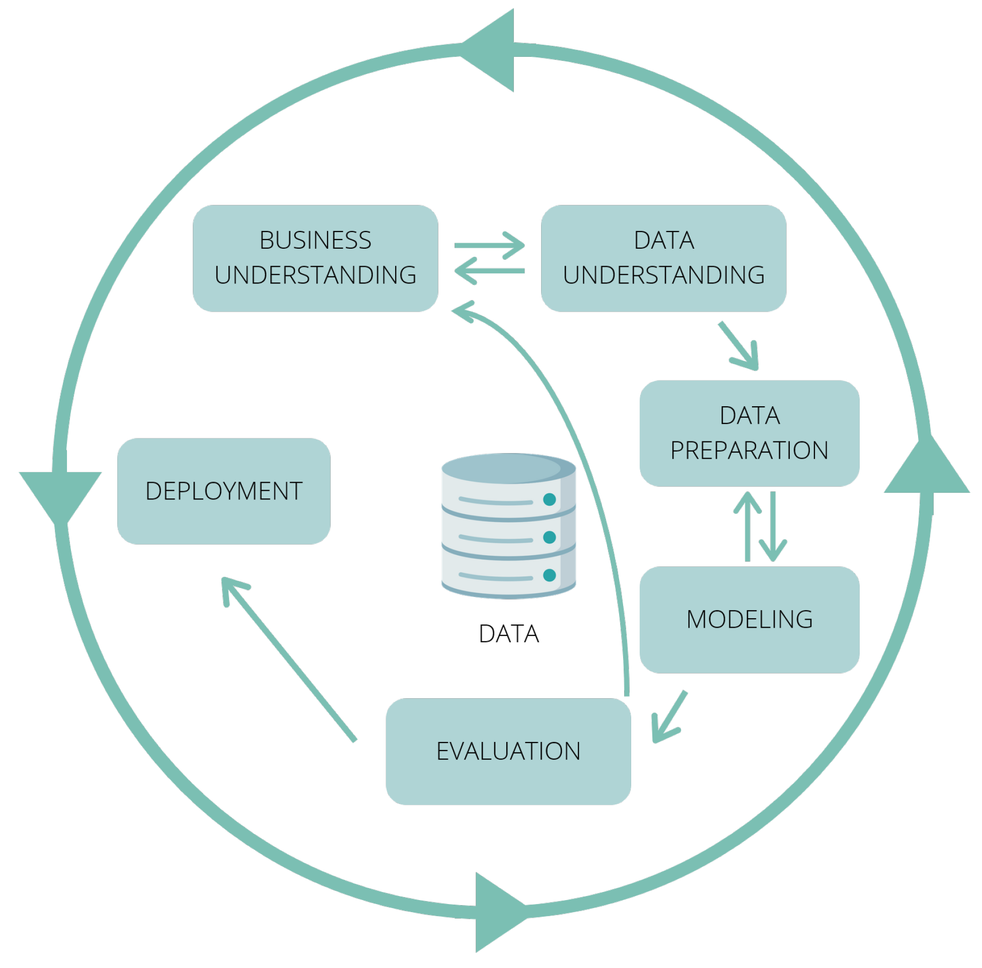
The DM process will follow the CRISP-DM Methodology (Cross Industry Standard Process for Data Mining), one of the most popular methodologies used in DM projects worldwide. CRISP-DM is a cyclic process, which is divided into six phases, namely,
Business Understanding,
Data Understanding,
Data Preparation,
Modeling,
Evaluation and
Deployment.
Figure 2 depicts the main stages of the CRISP-DM lifecycle.
The following subsections contain a detailed description of each stage of the CRISP-DM lifecycle.
3.1. Business Understanding
In recent years, consumers have begun to demand differentiated content from brands, and today they are thrilled by technology, looking for high standards of innovation, sophistication, and customisation. One of the strategies that companies can adopt to face this reality is the implementation of recommendation systems. By combining user profile information with information filtering and Machine Learning algorithms, recommendation systems have proven to be effective in providing users with a more intelligent and proactive information service.
In online shopping, a better recommendation system can have a direct effect on the revenue of the company, since the recommendations can have a significant impact on the purchase decisions of users [
43]. Thus, this study aims to improve many aspects related to recommendation systems and the way in which they affect human life.
At this stage of the project it is also important to analyze the main concerns and challenges regarding the understanding of the application domain. Ethical aspects are one of the main concerns surrounding recommendation systems. Research concerning the ethical issues related to these systems is divided into different scientific areas, since it usually focuses on particular aspects of the recommendation systems in a wide range of scenarios. At the same time, consumers are becoming increasingly aware of their rights and privacy concerns are beginning to emerge. In this way, most organizations exhibit some secrecy in disclosing the operational details of their recommendation systems due to the concerns about violating the rights of their costumers. This makes it difficult for researchers to acquire and discover more knowledge related to the functioning of these systems, thus hindering the progress of recommendation systems.
Having a clear understanding of the business objectives is an important effort in order to ensure that the DM process is carried out rigorously and that an efficient recommendation system is therefore achieved. Hence, the objectives that guided this study, are the following:
Increase the number of sales;
Improve company’s revenue;
Encourage engagement and activity on products and services;
Gain competitive advantage;
Calibrate user preferences;
Make personalized recommendations;
Find the recommendation algorithm and parameterization that leads to the highest overall performance of the product recommendation system.
The first five objectives are related to the recommendation business goals. The improvement of the quality of product recommendation systems is one of the most crucial aspects in the industry. This translates into an increment of customer’s satisfaction as well as in the improvement of the company’s profitability. The rest of the objectives set out are related to the objectives inherent to the DM process. These objectives will provide substantial insight into the product recommendation systems through the application and refinement of the DM techniques.
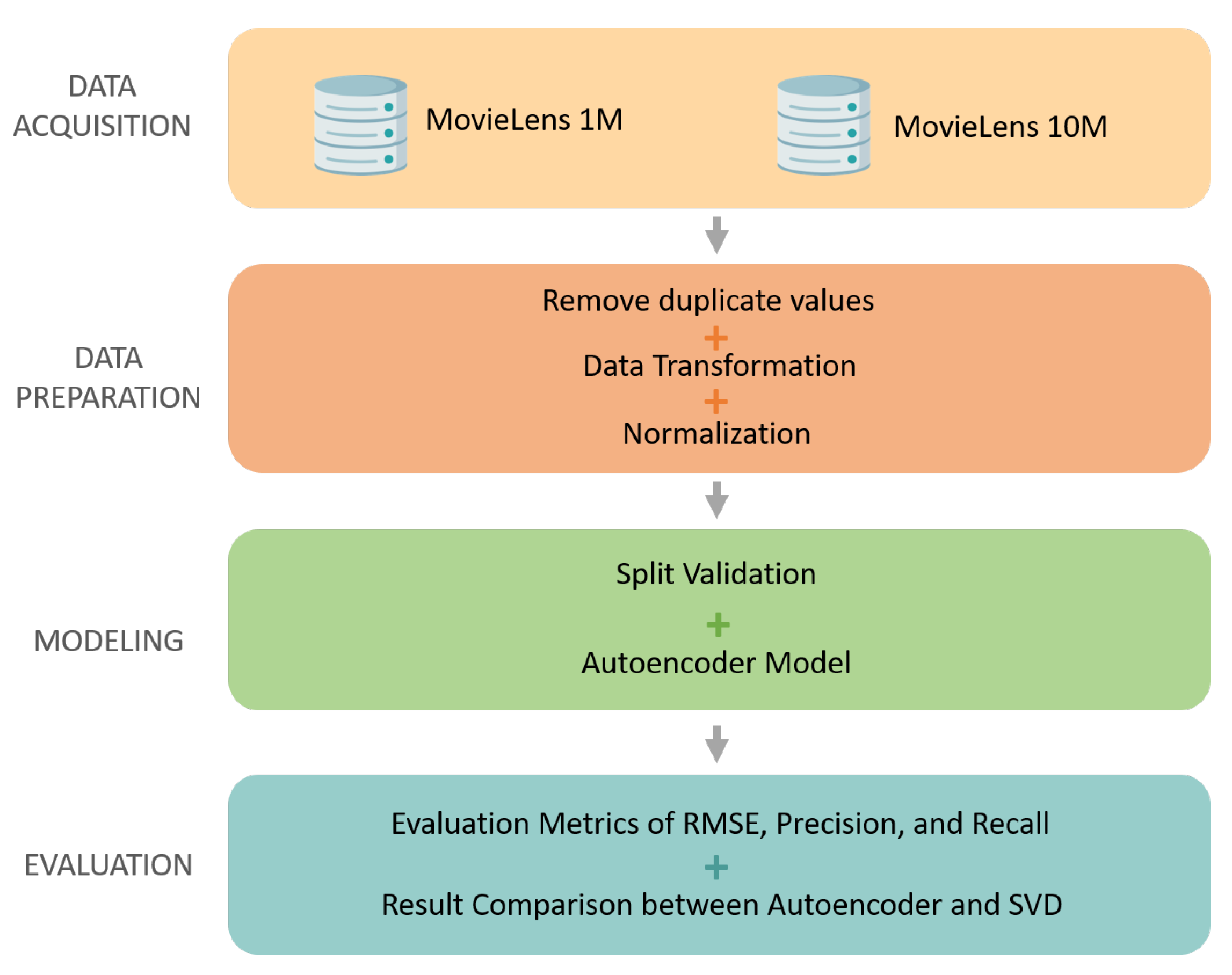
Hence, a project plan was designed to make an initial assessment of the techniques to be used in the further stages of the project.
Figure 3 details the steps to be executed in order to achieve the DM and business goals.
3.2. Data Understanding
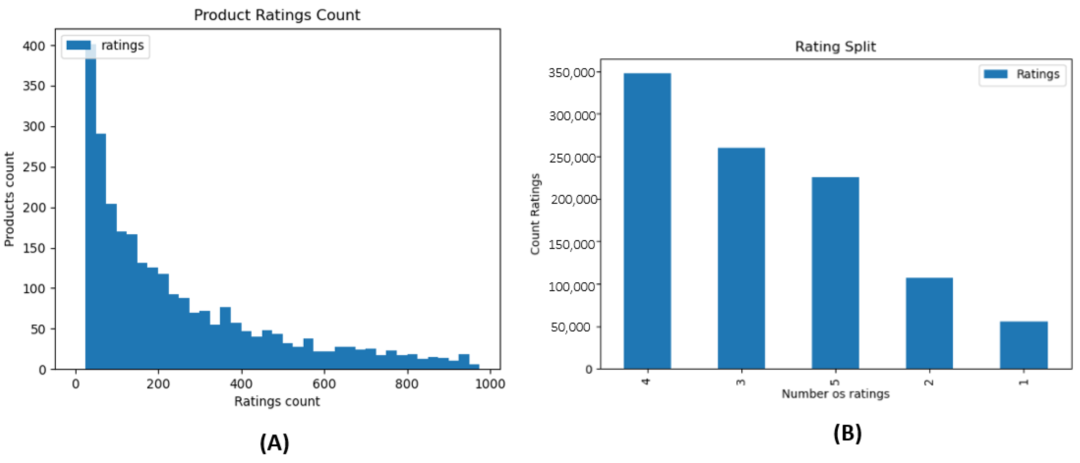
The data used in the present study corresponds to two MovieLens (ML) datasets. The first dataset, MovieLens1M, contains 1 million ratings made by 6040 users to 3706 movies, while the second one, MovieLens10M, contains 10 million ratings made by 69,878 users to 10,677 products. Each rating is an integer that varies on a scale from 1 to 5, where 1 is bad and 5 is excellent. For the purpose of this article, it is considered that the IDs of the movies are product IDs, since it is the goal of the recommendation system (recommend products).
Figure 4 shows the distribution of the quantity of products by a certain number of ratings (A) and the total number of ratings for each scale value [1–5] (B). The sparsity of the datatsets is 0.996. In addition, a dataset with 180249 products is also used, and its content consists in the combination of 4 different datasets found on the Kaggle platform called Amazon, Macys and Shop_norstrom (
https://www.kaggle.com/PromptCloudHQ/innerwear-data-from-victorias-secret-and-others), and Thrift Store (
https://www.kaggle.com/mateuspgomes/brazil-thrift-stores-data). As MovieLens datasets are the ones that have the product ratings, only those will be used for model training. The dataset of the products will be used in the end in order to retrieve the information related to the product and later pass it on to the user, as the final matrix produced by the model only contains the product id. Hence, when the time comes to give recommendations to the user, this ID will be located in the product dataset and its information will be returned.
3.3. Data Preparation
The importance of the data preparation stage can not be overlooked as the value of DM relies on it. This stage covers all the steps performed to construct and prepare the raw data into the final dataset in order to be fed into the data modeling stage. These tasks include data transformation and data cleaning. The first task carried out in relation to the two MovieLens datasets was a data treatment in which items with no more than 20 reviews and users who had not carried out more than 20 reviews were eliminated. The purpose of this selection was to improve the results, since collaborative filtering needs data to avoid problems. Then, all the duplicated instances were identified and removed to avoid ambiguity. In addition, all ratings were normalized, that is, the values were transformed into float and restructured so that they were between the range of [−1, 1]. After this step, the scale is no longer between [1–5] but between [0.20–1]. Finally, both MovieLens datasets were divided 80% for training and 20% for testing.
Table 1 shows the total number of users and items that remain after undergoing the data preparation stage.
3.4. Modelling
Ultimately, it is imperative to apply modeling techniques and provide their parameters to the learning dataset in order to determine which model performs best in the evaluation stage.
As mentioned earlier, this study will make use of an autoencoder. In this section, the autoencoder architecture used for the product recommendation system will be introduced. In addition, a brief explanation of autocoders and how they work will be presented as well as the parameters used to achieve the results featured in
Section 4.
3.4.1. Autoencoder Overview
An autoencoder is an unsupervised deep learning method that learns how to effectively compress and encode data, and then reconstructs data from a reduced encoded representation to a representation that is identical to the original input. In another words, an autoencoder is a neural network that applies back-propagation, setting the target values (outputs) to be equal to the inputs [
30,
44].
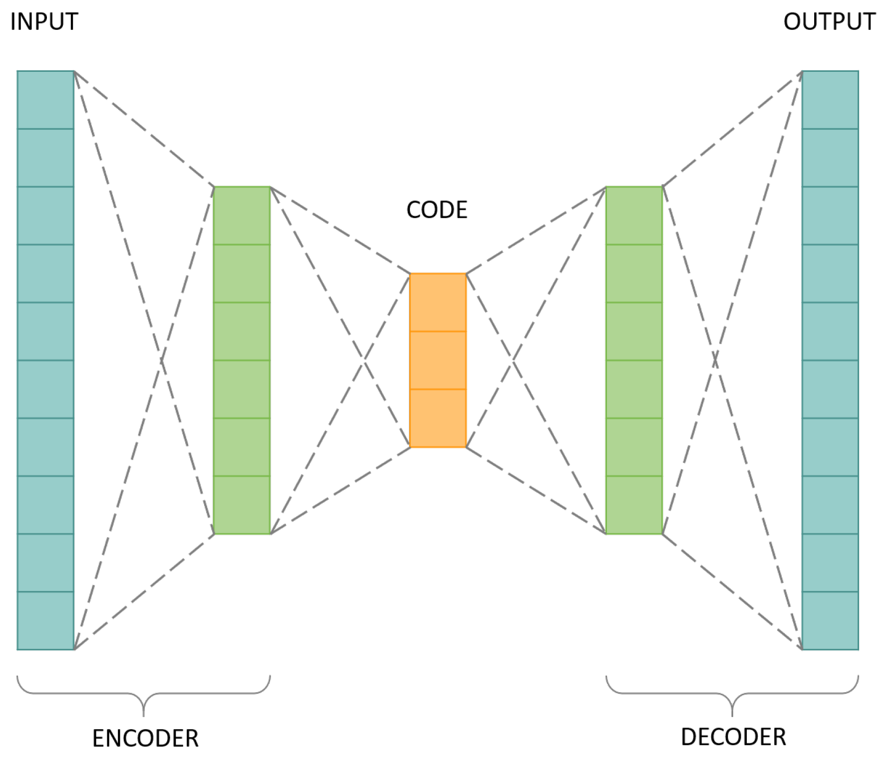
Hence, an autoencoder is typically a neural network of three layers, as demonstrated in
Figure 5.
The layers that constitute a basic autoencoder are: input layer, hidden layer, and output layer. The input layer and the hidden layer construct an encoder. The hidden layer and the output layer construct a decoder. Between these two, there is a code. Their description is the following the following:
Encoder has the function of compressing input information into a different latent space;
Code is a part of the network that represents the compressed input which is fed to the decoder;
Decoder does the reverse work and reconstructs the original information, moving from the latent space to the original information space.
The encoder encodes the high-dimensional input data
into a low dimensional hidden representation
by a function
f:
where
is an activation function,
n is the number of neurons in the input layer, and
m is the number of neurons in the hidden layer. The encoder is parameterized by a
weight matrix
W and a bias vector
[
27,
44].
Then, the decoder maps the hidden representation
h back to a reconstruction
by a function
g:
where
represents the decoder’s activation function. The decoder’s parameters are comprised of a bias vector
and a
weight matrix
[
27,
44].
The purpose of an autoencoder is to obtain
d dimensional representation of data such that an error measure between
x and
is minimized [
45].
Autoencoders have been widely used for its outstanding performance in data dimensionality reduction, noise cleaning, feature extraction, and data reconstruction [
46].
Over the years, recommendation systems have been extensively used to deliver personalized suggestions on products and/or services to users. Nonetheless, most recommendation systems still face challenges in dealing with the enormous volume and complexity of the data. In order to address this challenge, as discussed in
Section 2, several researchers have dedicated their investigation to improving recommendation systems by integrating deep learning techniques. The scientific literature contains recent studies that demonstrate a high efficiency of autoencoders in information retrieval and recommendation tasks. Hence, constructing a recommendation system based on an autoencoder would improve the accuracy of the recommendations due to a clearer understanding of the needs and characteristics of the users given its ability to learn the non-linear user-item relationship efficiently and to encode complex abstractions into data representations [
27].
3.4.2. Initialization of Parameters
By analyzing several articles related to autoencoders in the literature, it was possible to identify that each one uses a different set of parameters. Almost every author claims that, in a certain respect, a particular algorithm or parameterisation is better than another, which makes it difficult to choose between them. At the moment, it is difficult to find a detailed and objective comparison of the different approaches and the available results are sometimes paradoxical. Hence, the choice was made by “trial and error,” that is, by making an exhaustive experimenting with different criteria until the solution that best suits each person’s scenario was found.
Table 2 depicts the parameters chosen for the model.
The considerations and decisions that led to the parameters selected were the following:
For the loss function, because we are not dealing with a classification problem where binary cross-entropy can be used, the loss function used had to be the Mean Square Error (MSE);
The selection of the optimizer had to do with the fact that ADAM presents itself as one of the best, as it is very fast, requires little memory and is ideal for handling large amounts of data;
The dropout is only used during training, and is then automatically disabled during execution;
Finally, the choice of the activation function was based on the range to which the network values went, as well as the results of the experiments performed while running the autoencoder with other functions that were tested, but the loss and RMSE results were worse than the ones obtained with Tanh for the encoder layer, latent space and Linear for the output layer.
3.4.3. Architecture
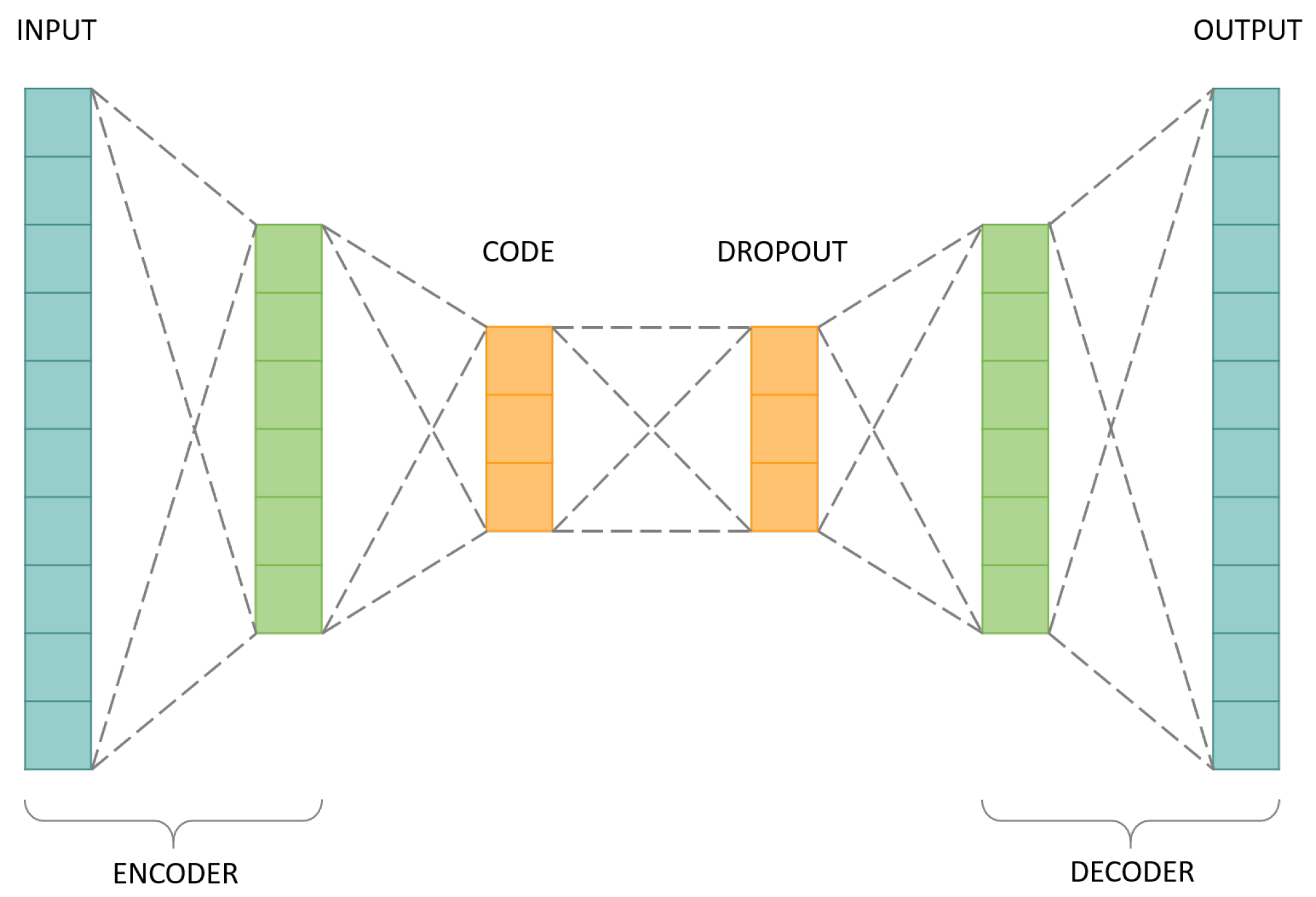
Figure 6 shows the final architecture used to obtain the results presented in
Section 4. The architecture is similar to the one shown in
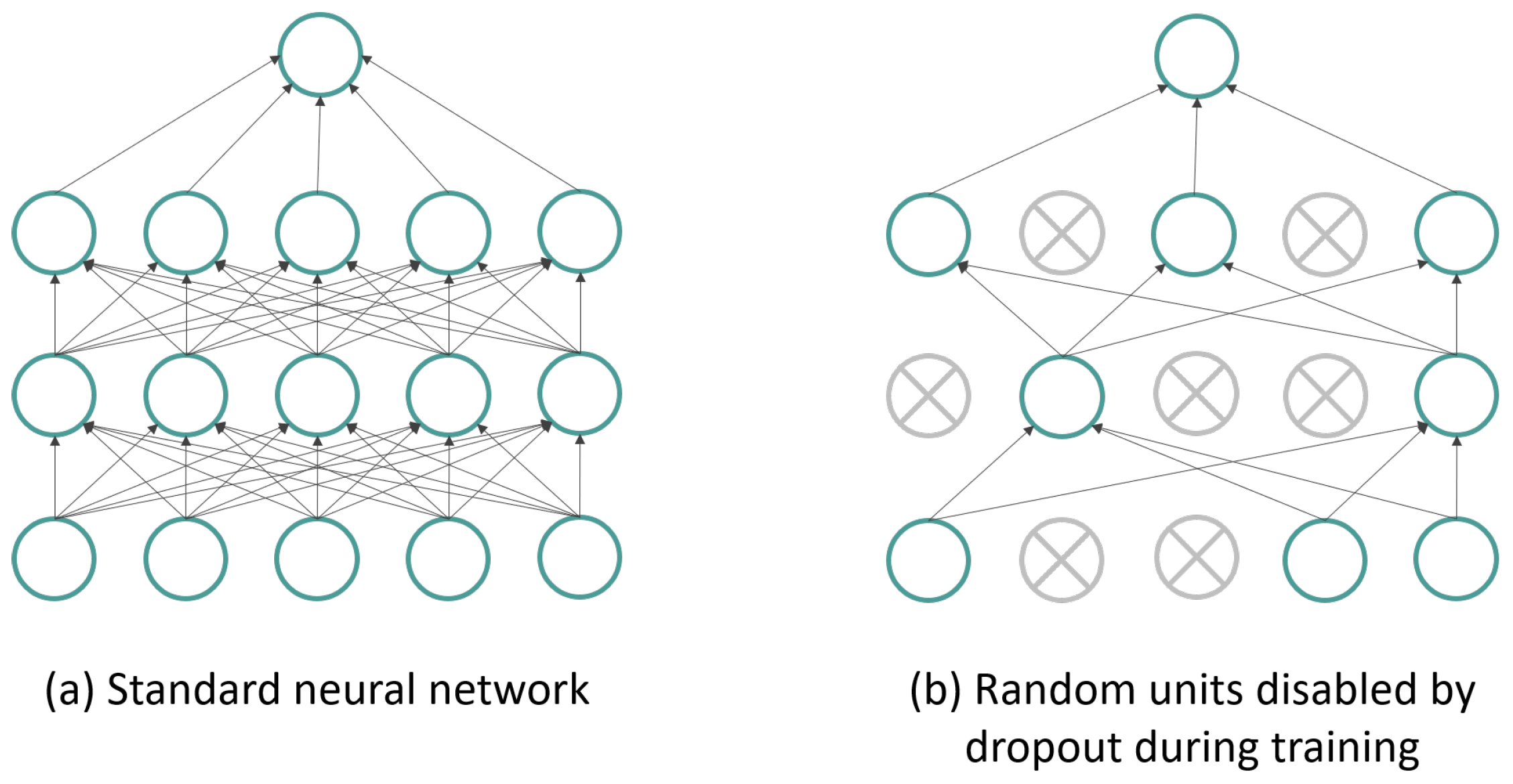
Figure 5, differentiating itself by the addition of another layer—the dropout layer. This layer prevents model overfitting and provides a way to efficiently combine several different neural network architectures exponentially. The term dropout refers to the removal of units, both hidden and visible, from the neural network [
47]. By dropping a unit, we mean temporarily removing it from the network, along with all its incoming and outgoing connections, as shown in
Figure 7.
3.5. Evaluation
The recommenders for online retailing shops can be evaluated through classification accuracy metrics. Further aspects that extend beyond the accuracy that recommendation systems typically need to be optimized are related to the technical performance and life-cycle of the system, such as responsiveness, scalability, reliability, maintenance, among others [
48,
49]. Coverage, confidence, trust, and security are other aspects that should be considered [
49,
50]. Measuring the different aspects of a recommendation system is a broad and demanding task beyond the scope of the study presented in this article. The metrics used to measure the accuracy of the recommendation system are divided into metrics of statistical precision and precision of decision support. The former evaluates the accuracy of a filtering technique by comparing the expected evaluations with the actual user evaluation, the others see the prediction procedure as a binary operation that distinguishes good items from those that are not good [
51]. That is, if we have a rating scale of 1 to 5, items that have a rating greater than 4 can be considered as relevant and the rest as irrelevant [
41].
In this model, the statistical accuracy metric used was the RMSE. This attaches greater importance to larger absolute errors:
where
is the expected evaluation for user
u in item
i,
is the actual evaluation of the user, and
n is the total number of evaluations in the set of items. The lower the RMSE, the more accurate the recommendation mechanism will be when predicting user reviews. The decision support accuracy metrics used were precision and recall. Precision is obtained from the fraction of recommended items that are relevant to the user [
41]. The calculation of this is presented in the following equation:
This represents the number of recommended items that are of interest to the user in relation to the set of all items recommended to them. The recall can be defined as the fraction of relevant items that are also part of the recommended item set [
41]. That is, it indicates the number of items of interest to the user that are recommended, as can be seen from the following equation:
4. Results and Discussion
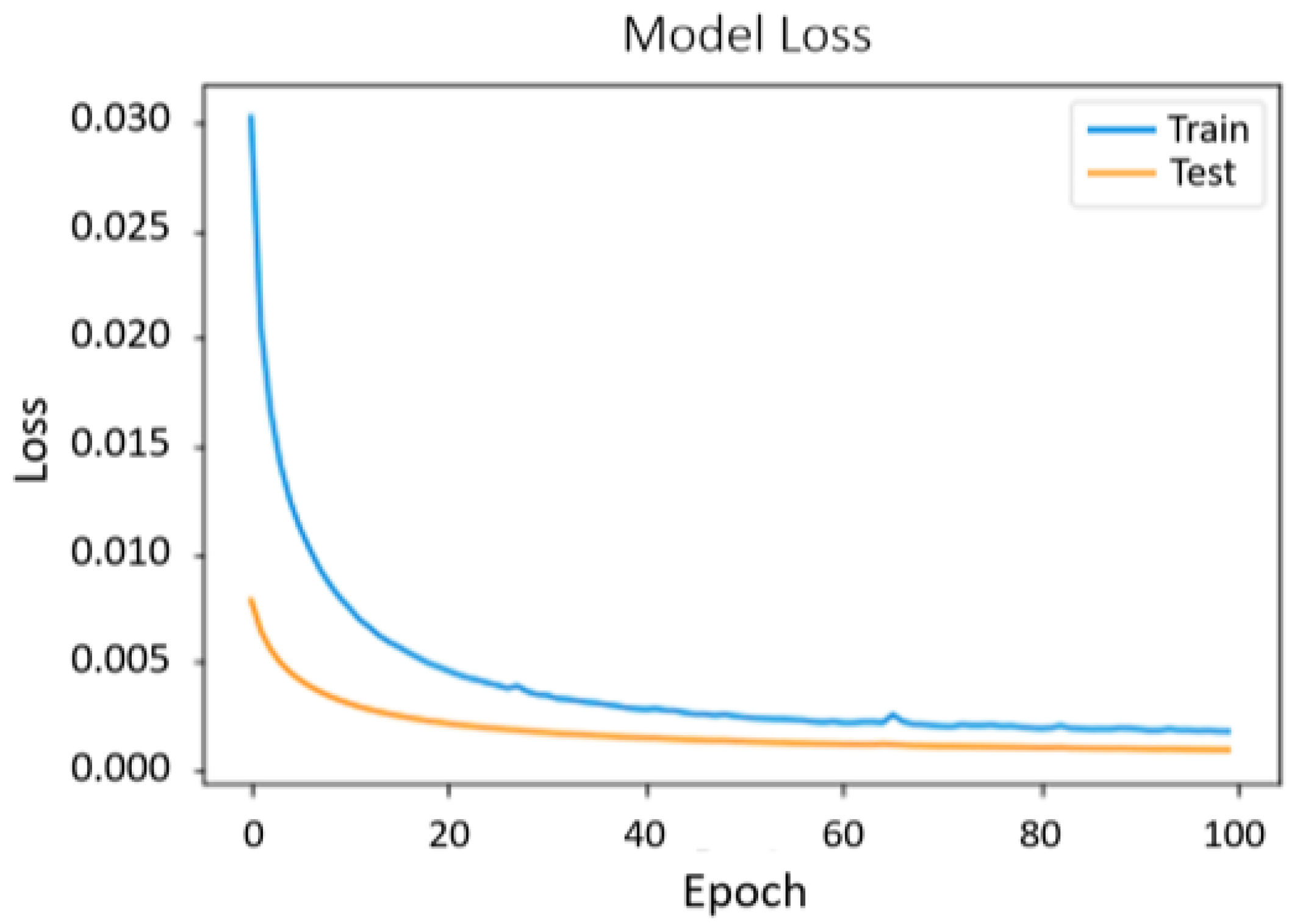
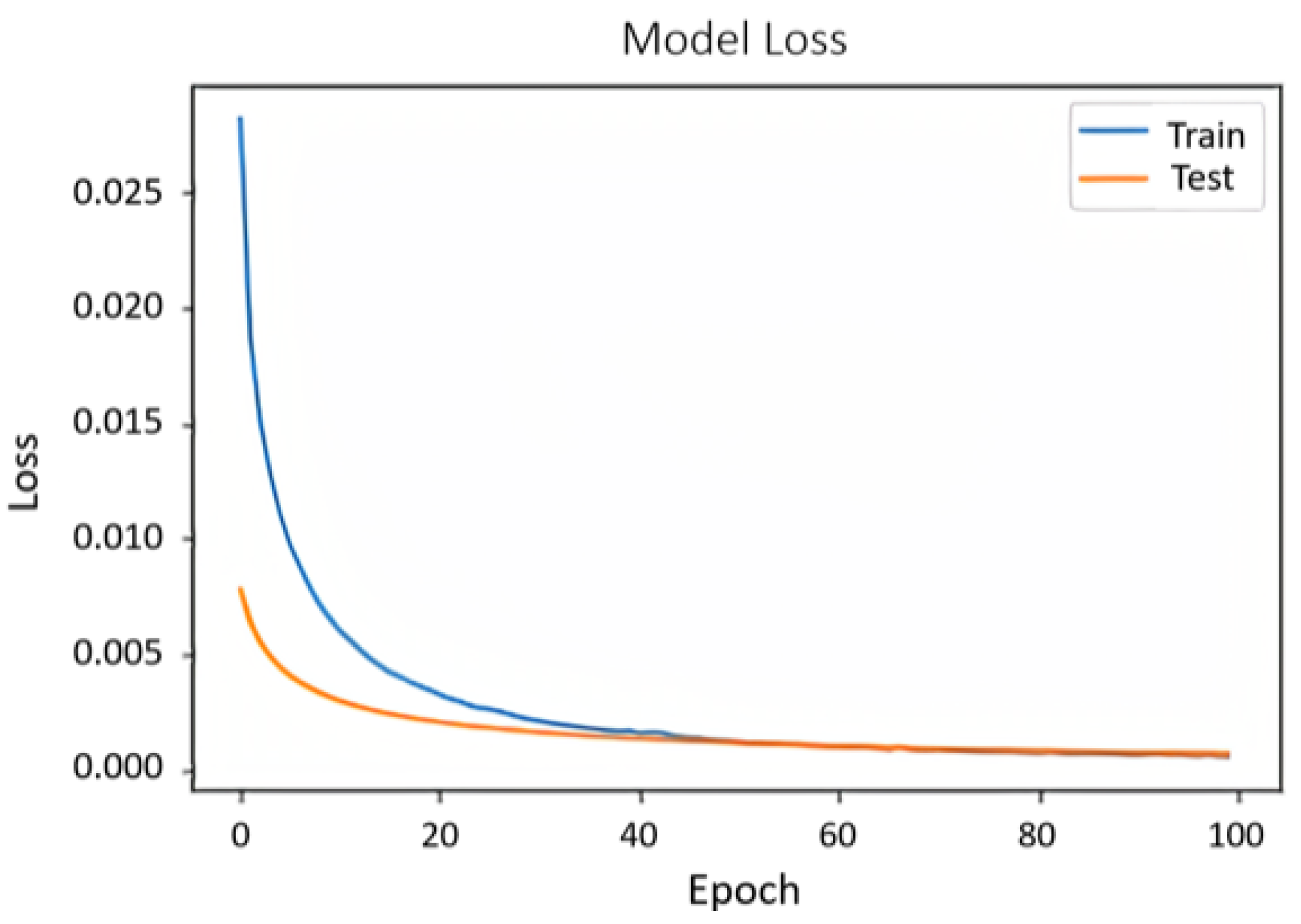
Figure 8 shows the performance of the model using the ML-1M dataset. In terms of loss and val_loss, they are decreasing over each epoch reaching a point where they begin to stabilize. There is no intersection of the loss curve with that of val_loss because when the dropout layer is added, it only acts on the training dataset, leading to the difference that can be observed between them. If this layer had not been added, the result would be an overfitted model as shown in
Figure 9.
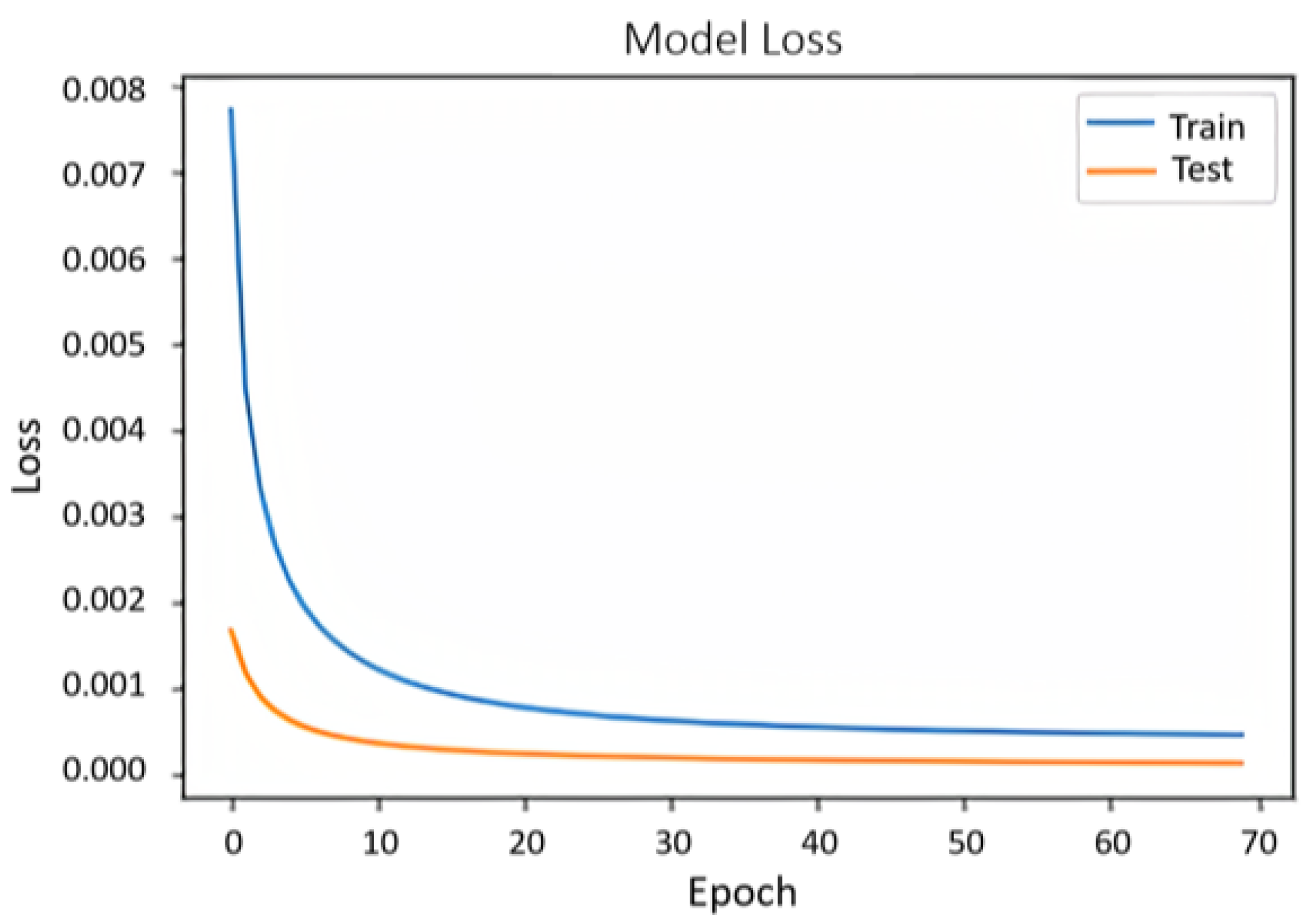
Figure 10 shows the loss model of the ML-10M dataset. When analyzing the figure, we can observe a behavior similar to that of
Figure 8, but the loss and val_loss present a lower value.
Figure 11 demonstrates the growth of precision and recall values throughout each epoch. The accuracy/recall graph of the ML-10M dataset has a structure similar to that shown in figure below. It was considered a threshold of 0.6 for both metrics. With these values and those of RMSE presented in
Table 3, it can be deduced that the model is having a good behavior towards the data, thus being able to provide recommendations, more accurate, that go against the interest of the user.
More layers were added to the autoencoder to check if the results could be better. In the experiment, only one layer was added and then, in a second phase, two layers were tested. The number of epochs and batch size remained the same and, with the exception of the number of neurons, all parameters maintained the same values. For each new layer, 1000 neurons were removed.
Table 3 shows the results obtained.
As we can analyze, with a greater number of layers in the autoencoder, for both datasets, the RMSE value tends to increase. Thus, it is not justified to consume more memory in order to use a greater number of layers if in the end we get a bigger error. Therefore, the choice of architecture presented in
Figure 6.
Table 4 shows the comparison of RMSE results between the created autoencoder model and the SVD. The SVD results were obtained using Surprise [
52] and the same data treatment was performed.
When analyzing these results, we can confirm that with the autoencoder we obtain better results compared to the SVD. Since the datasets are very sparse and we are using a collaborative filtering approach, we would expect problems to arise, but as we can see from the results, the autoencoder model has managed to overcome them. The fact that the RMSE decreases further in the ML-10 M suggests that the autoencoder had no difficulty in acting against a large set of data.
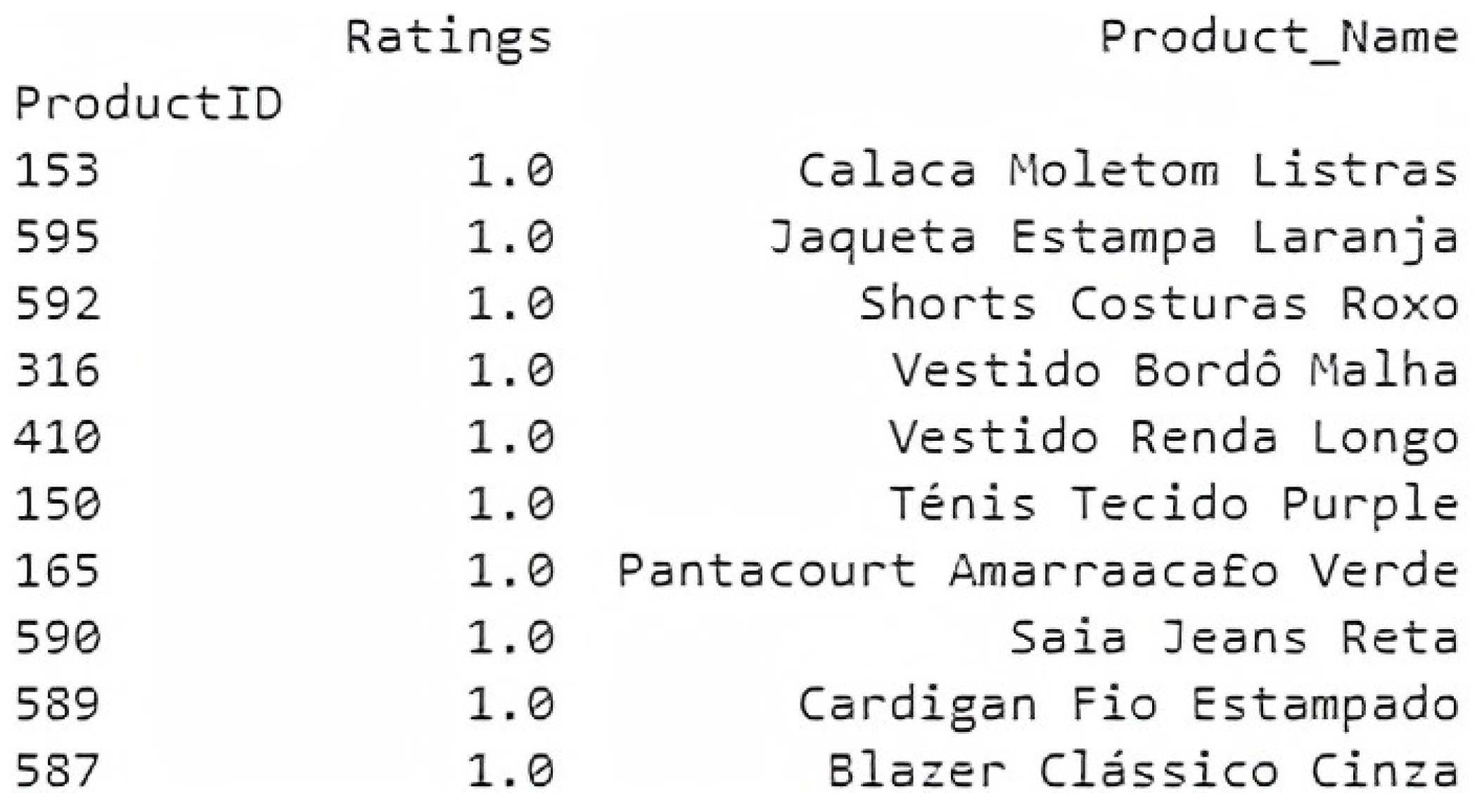
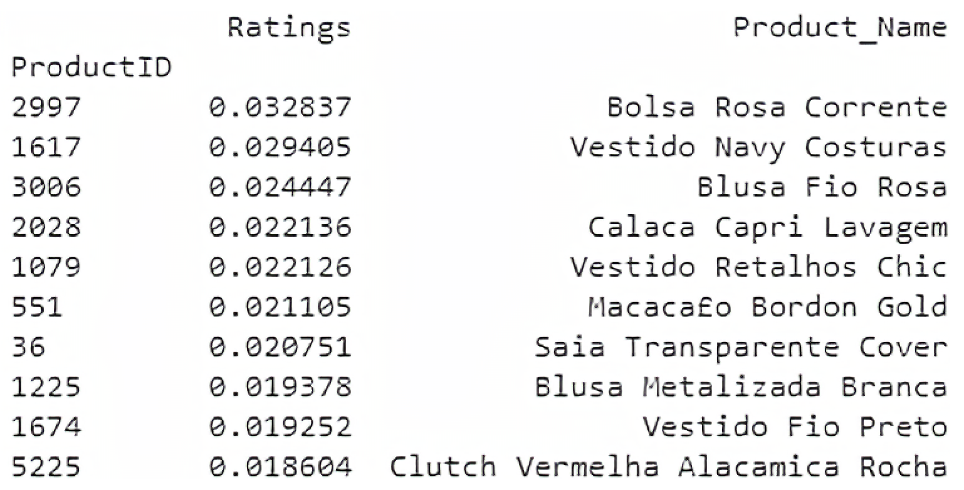
To conclude this evaluation of the results, in
Figure 12, 10 products are presented which the user has already evaluated with a high rating. These are displayed in order to have a short comparison with the 10 products suggested by the model, shown in
Figure 13.
5. Conclusions and Future Work
Retail organisations are under constant pressure to find new ways to respond to the progressive changes in the marketplace while at the same time meeting the increasingly challenging needs of their customers. Over the years, consumers have become more and more demanding, and today they are fascinated by all kinds of technology, seeking new ways of innovation, sophistication and a high degree of personalisation. Faced with this reality, organizations need to be prompt and effective in pursuing and creating new ways of attracting consumers through innovation in the way that they meet consumers’ needs and act before the market in order to increase sales and loyalty of their customers, thereby achieving competitive advantages.
One of the strategies that companies can adopt is the implementation of recommendation systems. The suggestion of products that meet the tastes and preferences of users makes recommendation systems an effective means of increasing revenues, offering companies a higher source of income and competitive advantage over their competitors.
Although recommendation systems have been around for quite some time and several companies and researchers have been working on the subject, as the vast majority of today ’s customers belong to a young group known as Generation Y or Millennials, which is characterized by an increased use of internet and technology, recommendation systems require constant innovation and improvement.
Hence, this study focus on finding effective ways to develop successful product recommendations. We found that the use of autoencoders for recommendation systems has shown great potential. In this paper, we present and implement an autoencoder model in order to obtain efficient product recommendations. In addition, we made a comparison of this approach with one of the techniques widely used for the purposes of recommendation systems, the Singular Value Decomposition (SVD). Although the SVD was faster in execution time, it was found that the autoencoder presented lower RMSE values. It was also possible to identify that the autoencoder performed better with a larger dataset, proving, once again, that collaborative filtering is more effective when faced with more data. The importance of using a dropout on the neural network was also presented, thus avoiding overfitting.
Collaborative filtering presents its limitations and ends up not working well if it is not faced with a reasonable amount of data, or if there are users with very different preferences from the others because this filtering is based on the similarity of users. In addition to these problems, this type of filtering is very closely linked to an external factor, the interaction of users with the platform that makes use of the product recommendation system, because it depends on the explicit feedback, that is, the user’s reviews of the products. As the method presented in this paper is based on this type of filtering, it also presents the same problems. In order to solve some of these vulnerabilities, in future work, it would be a good idea to use hybrid filtering to make greater use of different algorithms and to inspect if the results of the autoencoder would be better. Another idea would be to check how the model behaves in the face of new datasets. Finally, it would be interesting not only to make recommendations about products or services, but also to make recommendations for discount coupons, taking into account the products to which the users have expressed interest, thereby increasing the number of sales, the customer’s satisfaction, and the confidence bond with the company, while also offering competitive advantage.


