Article

NIR Hyperspectral Imaging Technology Combined with Multivariate Methods to Identify Shrimp Freshness

1
College of Information and Electrical Engineering, China Agricultural University, Beijing 100083, China
2
National Innovation Center for Digital Fishery, China Agricultural University, Beijing 100083, China
*
Author to whom correspondence should be addressed.
Appl. Sci. 2020, 10(16), 5498; https://doi.org/10.3390/app10165498
Submission received: 1 July 2020 / Revised: 27 July 2020 / Accepted: 5 August 2020 / Published: 8 August 2020
(This article belongs to the Section Electrical, Electronics and Communications Engineering)

Abstract

:
In this study, a hyperspectral imaging system of 866.4–1701.0 nm, combined with a variety of spectral processing methods were adopted to identify shrimp freshness. To gain the optimal model combination, three preprocessing methods (Savitzky-Golay first derivative (SG1), multivariate scatter correction (MSC), and standard normal variate (SNV)), three characteristic wavelength extraction algorithms (random frog algorithm (RFA), uninformative variables elimination (UVE), and competitive adaptive reweighted sampling (CARS)), and four discriminant models (partial least squares discrimination analysis (PLS-DA), least squares support vector machine (LSSVM), random forest (RF), and extreme learning machine (ELM)) were employed for experimental study. First of all, due to the full wavelength modeling analysis, three preprocessing methods were utilized to preprocess the original spectral data. The analysis showed that the spectral data processed by the SNV method had the best performance among the four discriminant models. Secondly, due to the characteristic wavelength modeling analysis, three characteristic wavelength extraction algorithms were utilized to extract the characteristic wavelength of the SNV-processed spectral data. It was found that the CARS algorithm achieved the best performance among the three characteristic wavelength extraction algorithms, and the combining adoption of the ELM model and different characteristic wavelength extraction algorithms obtained the best results. Therefore, the model based on SNV-CARS-ELM obtained the best performance and was elected as the optimal model. Lastly, for accurately and explicitly displaying the refrigeration days of shrimps, the original hyperspectral images of shrimps were substituted into the SNV-CARS-ELM model, thus obtaining the general classification accuracy of 97.92%, and the object-wise method was used to visualize the classification results. As a result, the method proposed in this study can effectively detect the freshness of shrimps.

1. Introduction

Shrimp is welcomed by consumers for its richness in zinc, selenium, copper, minerals, etc., high content of vitamin B12, low content of fat and sugar, delicious taste, fine texture, and high digestibility. Tissues of the shrimp are soft and rich in high-quality protein (20.6 g of protein per 100 g of shrimp meat). Astaxanthin in shrimp also has high nutritional value [1,2]. Besides, shrimp is rich in multiple microelements and vitamins necessary for the human body. Shrimp is the main ingredient of many high-end famous dishes in various countries around the world and can be cooked by diverse cooking methods. In addition, shrimp has a high medical value which has adjuvant therapeutic effects on the treatment of skin ulcers, hand and foot twitching, breast sores, neurasthenia, etc. Furthermore, to meet the demands of long-distance transportation and long shelf life in inland areas, shrimps are often processed and dried into seafood products such as dried small shrimps [3]. However, shrimp, as a seasonal and regional aquatic product, is prone to deterioration in quality during storage and transportation due to the effect of microorganisms and their enzymes [4]. The specific manifestations are as follows: the appearance of amines and other substances leads to the generation of volatile substances with peculiar smell; the presence of components such as formaldehyde leads to a reduction in muscle water-holding capacity and alters the textural properties of shrimp; the oxidation of tyrosine causes the color of shrimp body to change; protein and water changes in content and sensory status. With the change of shrimp quality, its edible value and safety decline, so it is not easy to store, and the short shelf life seriously affects the sales and circulation of the products [5]. Therefore, it is particularly important to determine the shelf life of shrimps in a timely and accurate manner [6,7].
Traditionally, methods of instrument analysis and artificial sensory evaluation were used to identify the freshness of shrimps. Instrumental analysis methods have poor reliability, take a long time, and are not repeatable, and artificial sensory evaluation cannot accurately reflect the freshness of all products in real-time [8,9,10,11,12]. In the last few years, a great number of research workers have implemented hyperspectral imaging techniques to detect the freshness of various products. Compared with the methods of instrumental analysis and artificial sensory evaluation, hyperspectral imaging technology is characterized by accurate prediction, low cost, and non-destructive testing, etc. Accordingly, it is widely used in the field of food freshness detection [13]. Dai et al. [14] built a numerical model of wavelet characteristics and criterion total volatile basic nitrogen (TVB-N) content by using a visible/near-infrared hyperspectral imaging (HSI) system combined with wavelet profiling methods and three regression algorithms, and eventually determined that the least squares support vector machine (LSSVM) model was the best model for shrimp TVB-N content inspection. The authors also developed an image processing method for TVB-N detection, which was capable of rapidly determining the TVB-N content of shrimp during refrigeration. Yu et al. [15] assessed the freshness of shrimp during refrigeration and depending on the TVB-N content of the shrimp, proposed that shrimps could be divided into two grades of freshness: fresh shrimp and stale shrimp. By using hyperspectral imaging technology, the spectral characteristics were taken from the raw hyperspectral data by a deep learning algorithm, the freshness of the shrimp was then determined by an LR-based deep learning algorithm. The study demonstrated that the classification accuracy of shrimp freshness by stacked auto-encoders logistic regression (SAEs-LR) reached 96.55% and 93.97% on the calibration and prediction sets, respectively. In addition, some scholars at home and abroad had studied the freshness of other aquatic products through near-infrared hyperspectral imaging technology. Sivertsen et al. [16] distinguished between fresh and freeze-thawed cod fillets by using VIS/NIR hyperspectral technology combined with machine vision, by which high classification accuracy was acquired and the freshness of each fillet could be determined and the number of frozen days could be evaluated with a precision of 1.6 days. Cheng et al. [17] used VIS/NIR hyperspectral imaging technology (400–1000 nm) combined with classifier and spectral pre-processing technology to distinguish fresh, frozen (4 °C, 7 days) and frozen-thawed (20 °C, −40 °C, 30 days) grass carp slices. Four kinds of classifiers were used to establish classification models and classifier analysis combined with hyperspectral imaging could quickly distinguish between frozen, frozen-thawed, and fresh fish slices. The modeling results showed that the classification accuracy peaked at 92.29% and hyperspectral imaging technology combined with classifier analysis had tremendous potential for online inspection. As a new generation of inspection technology, NIR hyperspectral imaging technology is developing well for aquatic product quality inspection as it can simultaneously obtain unique spectral and image information for each pixel of an object’s surface [18].
To our knowledge, studies have rarely utilized NIR hyperspectral imaging to accurately determine the shelf life of shrimp. Therefore, in this study, NIR hyperspectral imaging technology combined multivariate methods to identify the freshness of shrimp. The targets are as follows: (1) analyzing the changing trend and absorption peak distribution of full-band spectrum and average spectrum of white shrimps with different freshness; (2) selecting the best preprocessing method is identified by modeling and analyzing the full wavelengths with various preprocessing methods; (3) utilizing different characteristic wavelength extraction algorithms to extract the characteristic wavelengths of the spectral data processed by the best preprocessing method, and then various discriminant models are employed to identify the model performance of different characteristic wavelengths so as to work out the optimal model for freshness detection of white shrimps; (4) substituting the original random hyperspectral images into the optimal model to visualize the classification effect of white shrimp refrigerated for different days and the feasibility of the selected model is thus verified.

2. Materials and Methods

2.1. Sample and Sample Preparation

In total, 420 white shrimp of about 15 g of average weight were purchased from a seafood market in Chaoyang District, Beijing. All samples were placed in plastic bags, which were then placed in a clean white foam incubator filled with fresh crushed ice. There was a drip hole at the bottom of the incubator so that the crushed ice was converted into the water from the drip hole in the process of transportation. The special vehicle transported the samples to the laboratory within 1 h. After removing the head and tail, all samples were refrigerated in a 4 °C incubator, and 60 samples were tested every day for a total of 7 days.

2.2. Hyperspectral Imaging System

“GaiaSorter” near-infrared high spectrometer was used in the experiment. The system is equipped with electronic control mobile platform, 56 mm fixed focus near-infrared lens, unified light source consisting of four 200 W tungsten bromide lamps, computer box, hood, etc. The spectral range is from 866.4 nm to 1701.0 nm. The imaging mode of “GaiaSorter” near-infrared high spectrometer is line scanning. The imaging spectrometer forms an image of a line on the target each time and splits the light so that each spectral component corresponds to a pixel on the line array. As shown in Figure 1, the working mechanism can be described as follows: the experimental samples are placed on the electronic control mobile platform, and the hyperspectral cube information of the sample to be tested is obtained by the push-broom method.

2.3. Hyperspectral Image Acquisition and Correction

Half-hour preheating of the hyperspectral imaging system was essential prior to data acquisition to remove errors such as dark currents. Next, the SpecVIEW software was used (SpecView Ltd., Uckfield, UK) that comes with the system and executes a variety of tests, such as focusing. The exposure time of the system was finally determined as 0.09 s, the sampling interval was 3.37 nm, and the moving speed of the electronic control mobile platform was 0.55 cm/s. When the data were collected, 4 white shrimp samples for a group were placed on the electric mobile platform, and 15 hyperspectral images were collected every day; altogether 105 hyperspectral images were collected within 7 days. To avoid disturbance from outside light during data acquisition, a special glass baffle was used to shield the windows around the system. Besides, reflectance correction of the original hyperspectral images was required to reduce the influence of the experimental conditions [19], the correction formula is:
R = O H B H
In Formula (1): O represents the original hyperspectral image. H represents the all-black calibration image (camera lens cap closed, all four lights off, the black image captured by the camera, the theoretical reflectance is 0%). B represents the all-white calibration image (camera lens cap open, all four lights on, the white image captured by the camera on the whiteboard, the theoretical reflectance is 99%). R represents the corrected hyperspectral image.

2.4. Data Analysis

2.4.1. Spectral Data Extraction and Preprocessing

Because of the sophistication of the hyperspectral raw image data, it is essential to perform a sequence of processes on the hyperspectral raw image to ultimately extract the spectral data. As shown in Figure 2, the steps to extract the spectral data are as follows: (1) extracting edges of the white shrimp in the corrected hyperspectral images by using the Sobel operator; (2) binarizing the raw image to generate a mask, then separating the shrimp and the black standard plate to eliminate the black backdrop; (3) extracting the entire area of each white shrimp on the hyperspectral image as the region of interest (ROI), and then calculating the average reflectance of all pixels in the selected region as the spectral value of each white shrimp. In this process, the image segmentation was carried out on Matlab 2019a (The Math Works, Natick, MA, USA), while the computation of the average spectral values of all pixels in the ROI was performed on ENVI 5.3 (ITT Visual Information Solutions, Boulder, UT, USA).
Noise may be introduced during the data acquisition process due to interfering factors in some experimental conditions, it is essential to preprocess the raw spectral data to improve the modeling accuracy. In this research, three spectral preprocessing methods (Savitzky-Golay first derivative (SG1), multivariate scatter correction (MSC), and standard normal variate (SNV)) were employed to preprocess the raw spectral data, respectively.

2.4.2. Sample Set Division

In this study, a full 105 images were obtained, with 4 samples on each image and for a total of 420 samples. White shrimps with different refrigeration days were labeled as 1, 2, 3, 4, 5, 6, 7 as their respective sample labels. Before performing data analysis, the samples were divided into a calibration set and a prediction set. The model was trained by using calibration set data with known sample labels and followed by testing of model performance with prediction set data. Sample set partitioning based on be x-y distances (SPXY) was developed on the basis of the Euclidean distance method, which regards the spectral data as the independent variables and the sample labels as the dependent variables when calculating the distance between samples. Therefore, SPXY can be used to effectively establish the NIR quantitative model [20]. In this study, the average spectral data of white shrimps after being extracted the region of interest were divided into a 3:1 ratio by SPXY, that is, 315 samples were taken as the calibration set, and 105 samples were taken as the prediction set.

2.4.3. Selection Methods of Characteristic Wavelengths

Hyperspectral data have the characteristics of multiple bands, large data volume, and large redundancy. These characteristics will impact the model’s robustness, accuracy, and computational speed during subsequent modeling. Hence, it is crucial to extract the characteristic wavelengths with proper methods in the subsequent modeling analysis. In this study, random frog algorithm (RFA), uninformative variables elimination (UVE), and competitive adaptive reweighted sampling (CARS) were utilized to extract characteristic wavelengths.
RFA is a characteristic wavelength selection algorithm based on the idea of reversible jump Markov chain Monte Carlo (RJMCMC) model dimension conversion technology and model population analysis (MPA) [21]. The specific steps are as follows: (1) constructing an initial variable set V which contains M random variables; (2) constructing a candidate variable subset V1 which contains M1 random variables according to the initial variable set; (3) identifying the set of acceptable candidate variables V1 based on the probability of the root mean square error of cross-validation (RMSECV) such that V1 = V, and iterating it N times; (4) calculating the selection probability of each variable, and the greater the selection probability is, the more important the variable is to the model.
The purpose of UVE is to decrease the number of latent variables in the final model. It is a sort of algorithm based on the analysis of least partial square regression coefficients. The purpose is to get the least prediction error of the result by eliminating the variables of interference information and noise information [22], so characteristic wavelengths can be extracted. The steps are as follows: (1) performing PLS regression of the calibration set spectral matrix X(m × n) and sample label matrix Y(m × 1); (2) artificially generating normal distribution noise matrix R(m × n) and further combining it with X to form a matrix XR(m × 2n); (3) performing PLS regression on the matrix XR and Y, the factor number of the model is selected by leave-one-out cross validation (LOOCV), thus acquiring a regression coefficient vector r each time and m PLS regression coefficients in total to form a matrix B(m × 2n); (4) calculating the standard deviation S(r) and mean(r) of the matrix B(m × 2n) by column, and then calculating the stable value Ci = mean(ri)/S(ri), I = 1, 2, …, n; (5) taking the maximum absolute value of C in the interval [n+1,2n] and removing the variables of Ci < Cmax that correspond to the matrix X in the interval [1,n].
CARS is an effective method of data dimensionality reduction. First, Monte Carlo (MC) sampling is used to forcefully remove a part of the wavelength points. Then, select the wavelength points with large absolute values of regression coefficients by adaptive reweighted sampling (ARS) technique and delete the wavelength points with small weighting coefficients. Meanwhile, by utilizing cross-validation, the subset with the minimum RMSECV value is selected, so the smallest variable subset is the best subset [23]. The optimal combination of variables can be found out effectively, and the variable with a larger absolute regression coefficient can be selected in multiple Monte Carlo operations to achieve the purpose of variable dimensionality reduction.

2.4.4. Discriminant Model and Performance Evaluation

Partial least squares discrimination analysis (PLS-DA), as a supervised discriminant analysis method, is a high-dimensional linear discriminant analysis model using partial least squares regression (PLSR) [24]. In addition, PLS-DA is an algorithm based on the relationship between spectral data and sample characteristics. It converts the data of the calibration set into latent variables to determine the sample label of the prediction set. Therefore, the number of latent variables (LV) is a key parameter of PLS-DA. A too-small number of latent variables will result in too low model accuracy, while too many latent variables will lead to overfitting. This study chooses ten-fold cross-validation to determine the optimal number of latent variables.
The key of least squares support vector machine (LSSVM) is to find all the support vectors from which the optimal separation hyperplane can be obtained [25]. LSSVM uses the least-squares linear system as a loss function instead of the quadratic planning method as a loss function of the SVM and changes the inequality constraint in the SVM to an equation constraint, which significantly simplifies the calculation of the Lagrange multiplier alpha. SVM is a quadratic programming (QP) problem, while LSSVM is a problem of solving linear equations. LSSVM has two important parameters that affect the model’s ability to generalize, namely the penalty coefficient (c) and kernel range (σ). In general, the requirements of the model accuracy and complexity on the parameters (c, σ) are contradictory. In practice, the grid method should be used to select the optimal model parameters.
Random forest (RF) is a classifier that uses several trees to train and predict, it is a special bagging method that uses decision trees as a model in bagging. Random forest randomizes the use of variables (columns) and data (rows) to generate many classification trees, each of them is an independent judgment branch, they are independent of each other [26]. Random forest improves the prediction accuracy without significant increase in the amount of calculation, and is insensitive to multivariate linearity. The missing data and unbalanced data are more robust, which can effectively predict the role of up to thousands of variables. When a new object is classified and discriminated based on certain attributes, each tree in the random forest will give their own classification choice, and then “vote”, by means of which the overall output of the forest will be the classification option with the most votes. Compared with a single decision tree algorithm, it produces a better classification effect, and is not prone to overfitting.
Extreme learning machine (ELM) or “over-limit learning machine” is a model based on a feed-forward neural network (FNN) machine learning system or method for solving supervised and unsupervised learning problems [27]. ELM is deemed to be a unique FNN or an enhancement to the FNN and its backpropagation (BP) algorithm. The traditional neural network learning algorithm needs to be set in a lot of parameters in the training model, while the ELM only needs to be set in the number of hidden layer neurons (L) and the excitation function. The process of algorithm execution does not need to be iterated and the input weights and hidden element offsets are randomly generated. The connection weight (β) between the hidden layer and the output layer generates the only solution by calculating the equations. Therefore, ELM improves the learning speed of the forward neural network without being trapped into the local minimum value or overfitting.
The reliability and accuracy of the predictive model performance are assessed by the correct classification rate (CCR), which is calculated as follows:
C C R = T P P
In Formula (2): CCR represents the correct classification rate, TP represents the number of correctly classified samples, and P represents the total number of samples.

3. Results and Discussion

3.1. Original Spectral Analysis

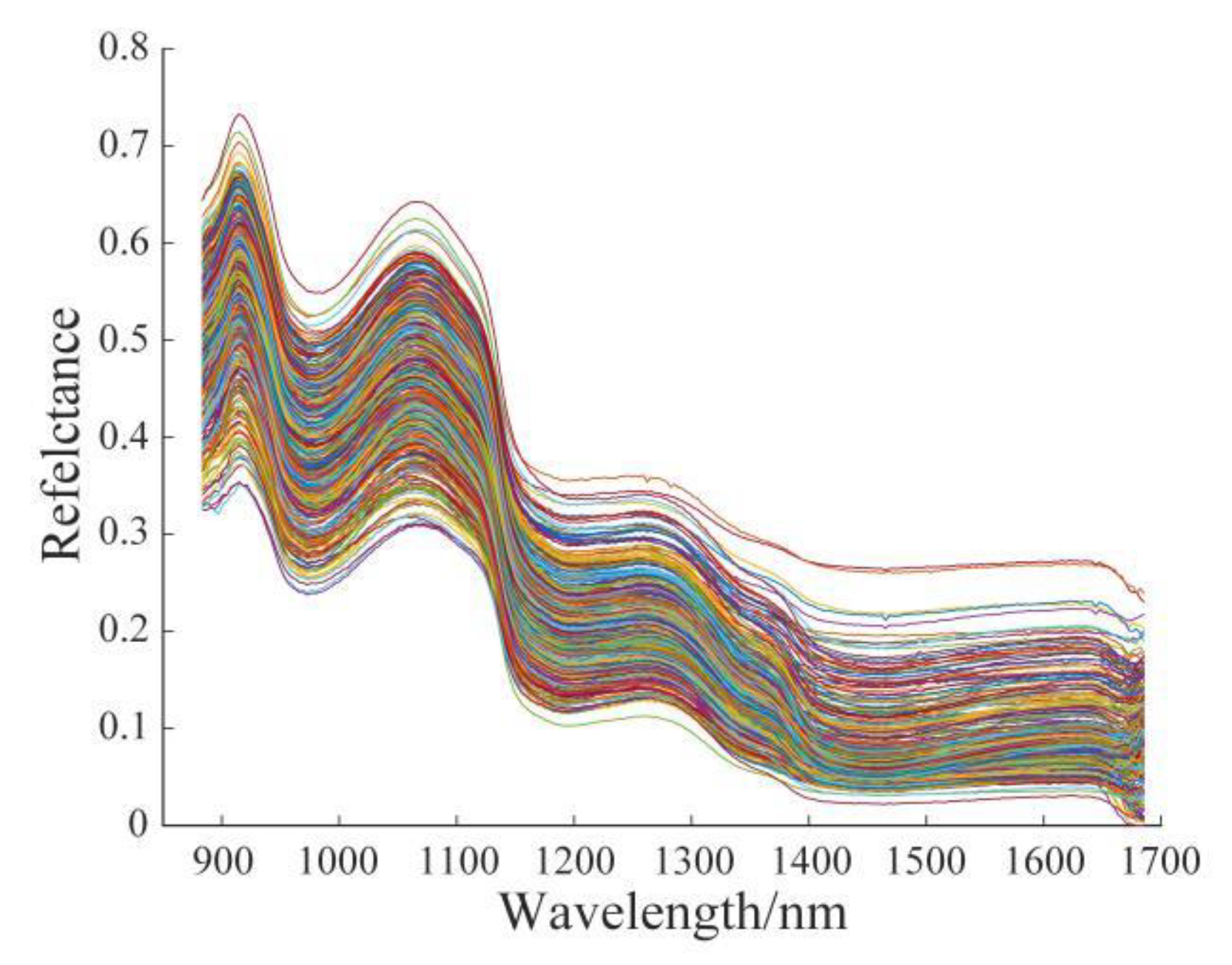
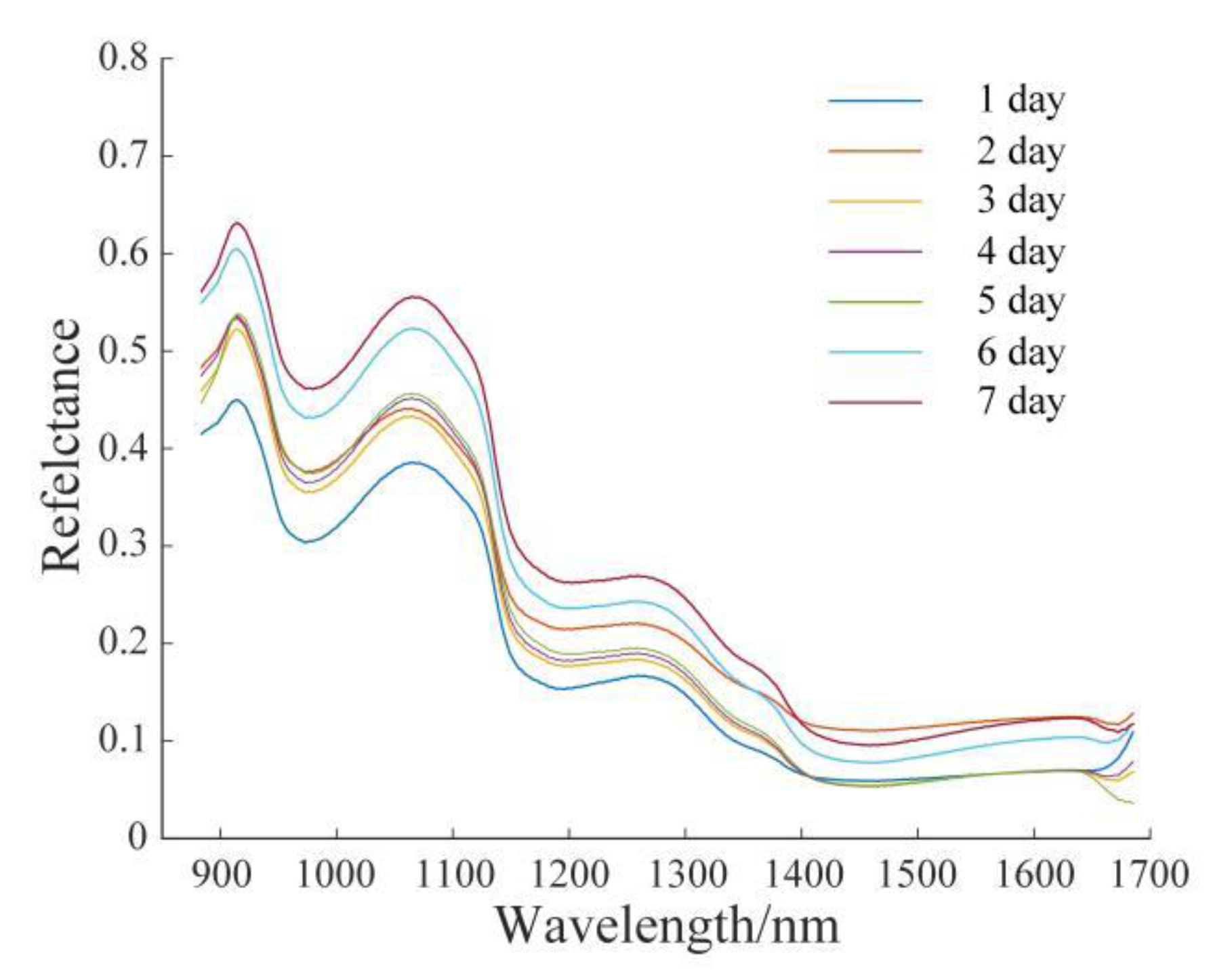
Figure 3 shows the original spectral curves for all samples. Due to the influence of noise, there are obvious distortions in the front and posterior parts of the original spectral curve, so five wavelengths were truncated in the front and back, respectively, and the spectrum with a wavelength range of 883.6–1685.3 nm was selected. In total, 244 wavelengths were selected for analyses. It can be seen from the figure of original spectral curve that the maximum reflectance is not higher than 0.75 in the range of 883.6–1685.3 nm. The 914.6-nm absorption peak band corresponds to the second overtone stretching of C-H, which is caused by the molecular structure CH2. The 1064.8-nm absorption peak band corresponds to the second overtone stretching of N-H, which is caused by the molecular structure RNH2. The 1259.0-nm absorption peak band corresponds to the second overtone stretching of C-H, which is caused by the molecular structure CH3. Figure 4 shows the average spectral curve over 7 days. The trends of the spectral curves of white shrimps with different refrigeration days are similar, but in the range of 1150–1300 nm. As can be observed, the spectral reflectance of white shrimps differs significantly in different days and as the refrigeration days increase, the reflectance rises gradually. Overall, the difference between the average spectral curves on day 1 and day 7 is the largest one, while the difference between the average spectral curves on days 2, 3, 4, and 5 is tiny.

3.2. Modeling Analysis Based on Full Wavelength

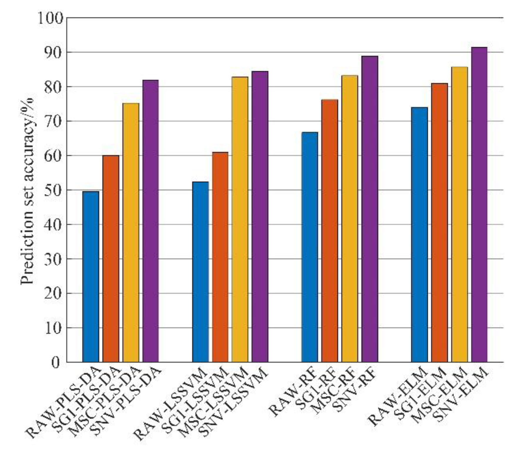
To determine the optimal combination of preprocessing methods and models, raw spectral data and spectral data preprocessed by SG1, MSC, and SNV were entered into PLS-DA, LSSVM, RF, and ELM discriminant models for comparison. Figure 5 displays the accuracy of the prediction set of the above full wavelengths preprocessing methods combined with PLS-DA, LSSVM, RF, and ELM discriminant models, in which RAW represents the original spectral data. The analysis yields that the SNV-processed spectral data modeling accuracy is the highest and the prediction set has higher accuracy than that of the other two preprocessing methods and the original spectral data. This result arises from the differences within the samples and other factors. The hyperspectral instrument used in this experiment may lead to light scattering and further generate noise. SNV uses the average value and standard deviation as the correction parameters, which eliminates the differences within the samples and light scattering to a large extent [28].

3.3. Selection Results of Characteristic Wavelengths

When the data dimension is large, the information is redundant, the subsequent modeling is relatively slow and the robustness is low. Therefore, it is essential to find out those characteristics that are most effective for classification identification among many characteristics, which should have a large quantity of identification information to make the discriminant models easy to classify and should have reliability and independence, so as to achieve the compression of the characteristic space dimension. The meaning of characteristic extraction is such that heterogeneous pattern points are farther apart in the minimum dimensional characteristic space (larger distance between classes), while similar pattern points are closer together (smaller distance between classes). Lastly, the SNV-processed spectral data is chosen for characteristic wavelengths extraction, and then the final model combination is determined according to the modeling analysis of the characteristic wavelengths. In this experiment, RFA, UVE, and CARS were utilized to extract characteristic wavelengths from the SNV preprocessed spectral data, respectively.
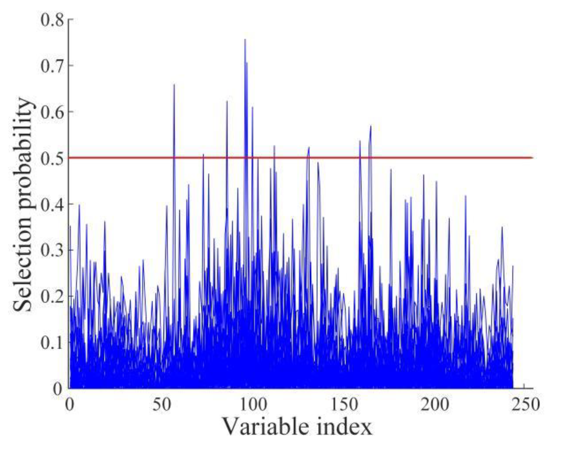
Figure 6 shows the selection probability of each characteristic wavelength extracted by RFA, which is acquired by setting the number of iterations N to 1000 and the number of initial variable M to 2. Since the random frog algorithm is based on Monte Carlo (MC) thought, in order to approximate the optimal solution, it needs to be run multiple times and the results are statistically calculated. A total of 50 RFAs were run in this experiment, and the average value of the 50 runs was used as the basis for the final characteristic wavelengths selection. As can be observed from the figure, the majority of the variables have a low probability of being selected, and only a small number of variables have a high probability of being selected. The experimental threshold is 0.5, which is represented by a red horizontal line, and 11 variables whose probability exceeds the threshold were selected as characteristic wavelengths. Table 1 shows the characteristic wavelengths and the corresponding molecular vibration extracted by RFA [29]. The extracted characteristic wavelengths account for 4.51% of the full wavelengths.
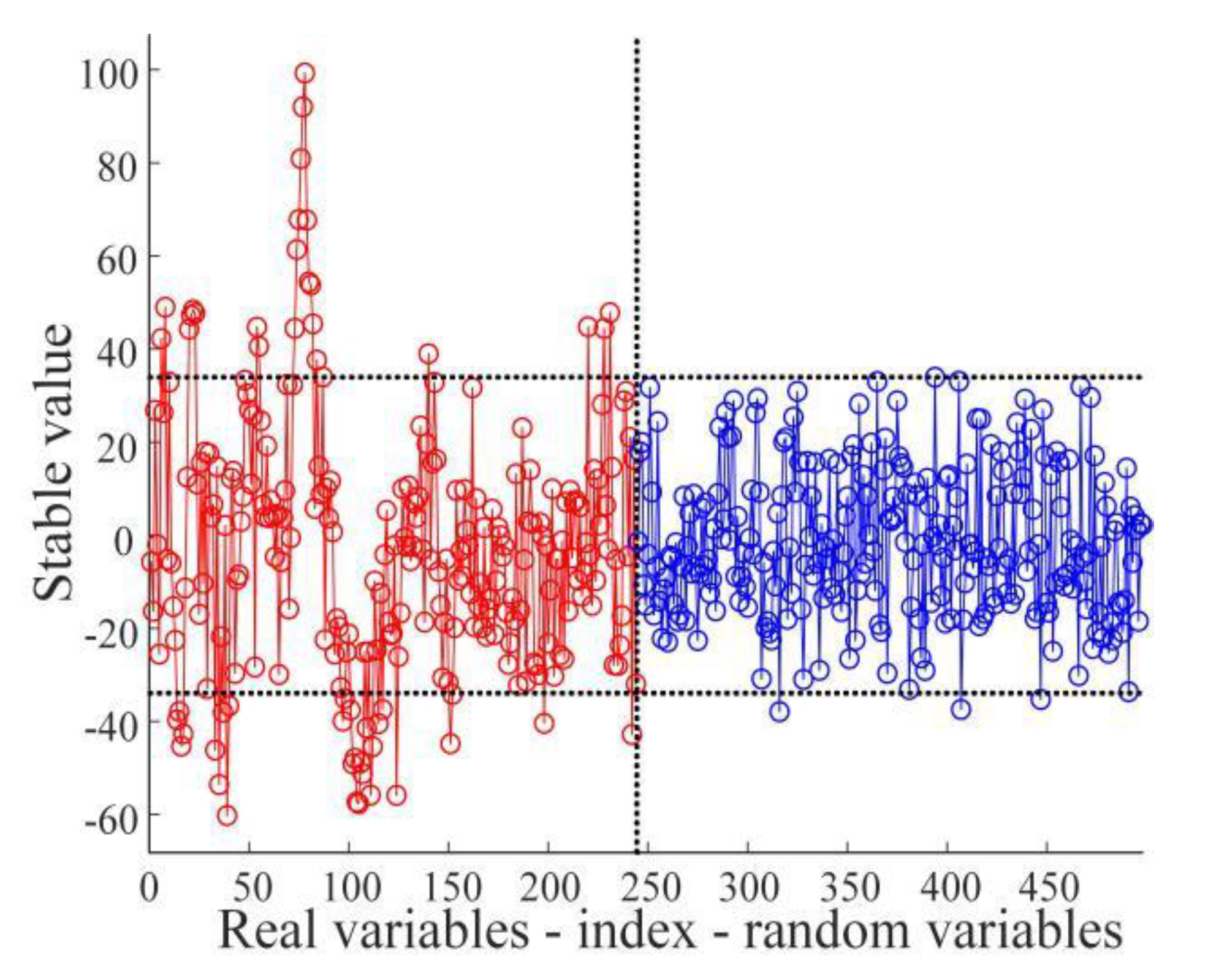
Figure 7 is the stability analysis of UVE. The number of LOOCV is 315, and the optimal factor number is 10, and the number of wavelengths of random noise added is 244. The vertical black dotted line shows the spectral wavelength variables stability distribution curve to the left and the introduced 244 system noise variables stability distribution curve to the right. The threshold for the stability of variables in this experiment has an upper and lower threshold of ±33.9396, which are represented by two horizontal black dotted lines. The 192 wavelength variables between the two thresholds are non-information variables that can be eliminated, and the 52 wavelength variables that exceed the threshold are information variables. Finally, 52 characteristic wavelengths were selected by UVE for subsequent modeling analysis. Table 2 shows the characteristic wavelengths and the corresponding molecular vibration extracted by UVE [29]. The extracted characteristic wavelengths account for 21.31% of the full wavelengths.
Figure 8 shows the results of CARS after 100 times of operation. The curve (a) shows an exponential decay, which means that with Monte Carlo (MC) sampling, the number of selected variables decreases, and the algorithm forcibly removes some wavelength points. The curve (b) is the trend diagram of RMSECV, from which the trend of slow decline, gradual rise, and then rapid rise can be seen. When the number of ARS is 73, the RMSECV value reaches the smallest, indicating that the redundant information in the spectrum is eliminated. The curve (c) represents the regression coefficient path, where “*” represents the sampling times when the lowest point of residual corresponds to the lowest RMSECV value, by means of which the optimal subset is determined. Finally, seven characteristic wavelengths were selected by CARS for subsequent modeling analysis. Table 3 shows the characteristic wavelengths and the corresponding molecular vibration extracted by CARS [29]. The extracted characteristic wavelengths account for 2.87% of the full wavelengths.
In summary, three characteristic wavelength extraction algorithms extracted different quantities of wavelengths, among which CARS extracted the least number of characteristic wavelengths and UVE extracted the largest number of characteristic wavelengths. During the degradation of proteins and fats, white shrimp with different days of refrigeration produce significant amounts of C-H, N-H, and H2O. The characteristic wavelengths extracted by RFA, UVE, and CARS are highly correlated with freshness.

3.4. Modeling Analysis Based on Characteristic Wavelengths

The samples for the calibration and prediction sets utilized in this subsection are the same as those used in the full wavelength modeling-based analysis. To further choose the optimal model combination, this study combines SNV preprocessed spectral data with different characteristic wavelength extraction algorithms and the data corresponding to the extracted characteristic wavelengths were input into PLS-DA, LSSVM, RF, and ELM discriminant models. Table 4 shows the results of modeling analysis of different characteristic wavelength extraction algorithms combined with PLS-DA, LSSVM, RF, and ELM discriminant models. It is evident from the analysis of this table that (1) by comparison with the results of the analysis based on full wavelength modeling, it is observed that the four discriminant models combined with different characteristic wavelength extraction algorithms yield good overall classification results. (2) The CARS combined with each discriminant model performs best, different characteristic wavelength extraction algorithms (RFA, UVE, CARS) combined with the same discriminant model, the CARS algorithm combined with the discriminant model acquires the highest accuracy of the calibration set and prediction set, indicating that CARS can eliminate the full wavelength redundancy to the greatest extent possible and preserve usable information, thus improving the accuracy of the model, while RFA and UVE do not show this effect. (3) The same characteristic wavelength extraction algorithm combines four discriminant models (PLS-DA, LSSVM, RF, ELM). Among them, the ELM model combined with the characteristic wavelength extraction algorithm achieves the best performance (the accuracy of both calibration and prediction sets in the ELM model exceeds 95%), which indicates that the most efficient data classification can be achieved by ELM.
In summary, the SNV-CARS-ELM model has the best classification performance (the calibration set and prediction set have the highest accuracy, 99.05% and 98.10%, respectively). Therefore, it is chosen as the optimal classification model.

3.5. Visualization of White Shrimp on Different Refrigeration Days

In order to intuitively judge the white shrimps of different refrigeration days, it is essential to categorize the pixels of hyperspectral images and visualize the categorization effect. In the previous studies, a number of researchers utilized object-wise and pixel-wise methods to implement the visualization of classification effects. The object-wise method treats the whole object as a pixel and employs the average spectral data of all pixels as the spectral data of the sample. The pixel-wise method takes the predicted category of single-point pixel data as the value of each pixel in the sample.
Baek et al. [30] utilized variable importance in projection (VIP) to extract characteristic wavelengths and then used PLS-DA to build the model. Viable soybean seeds and the non-viable soybean seeds were categorized and visualized based on the pixel-wise method and the object-wise method, and it was shown that the pixel-wise method of classification cannot detect the non-viable seeds with high precision, but the object-wise method achieved better classification results. In the actual grading of freshness, the degree of degradation of protein and fat varies with the number of days of refrigeration. If the pixel-wise method is employed, some white shrimps with similar spectral characteristics but different refrigeration days may be misjudged, while the use of the object-wise method can avoid the defect. Moreover, the freshness of shrimps is a concept related to the whole shrimp. Therefore, each pixel in the images of white shrimps cannot be considered to represent the freshness of the shrimp. Thus, the present research employed the object-wise method to achieve visualization of white shrimp with different days of refrigeration.
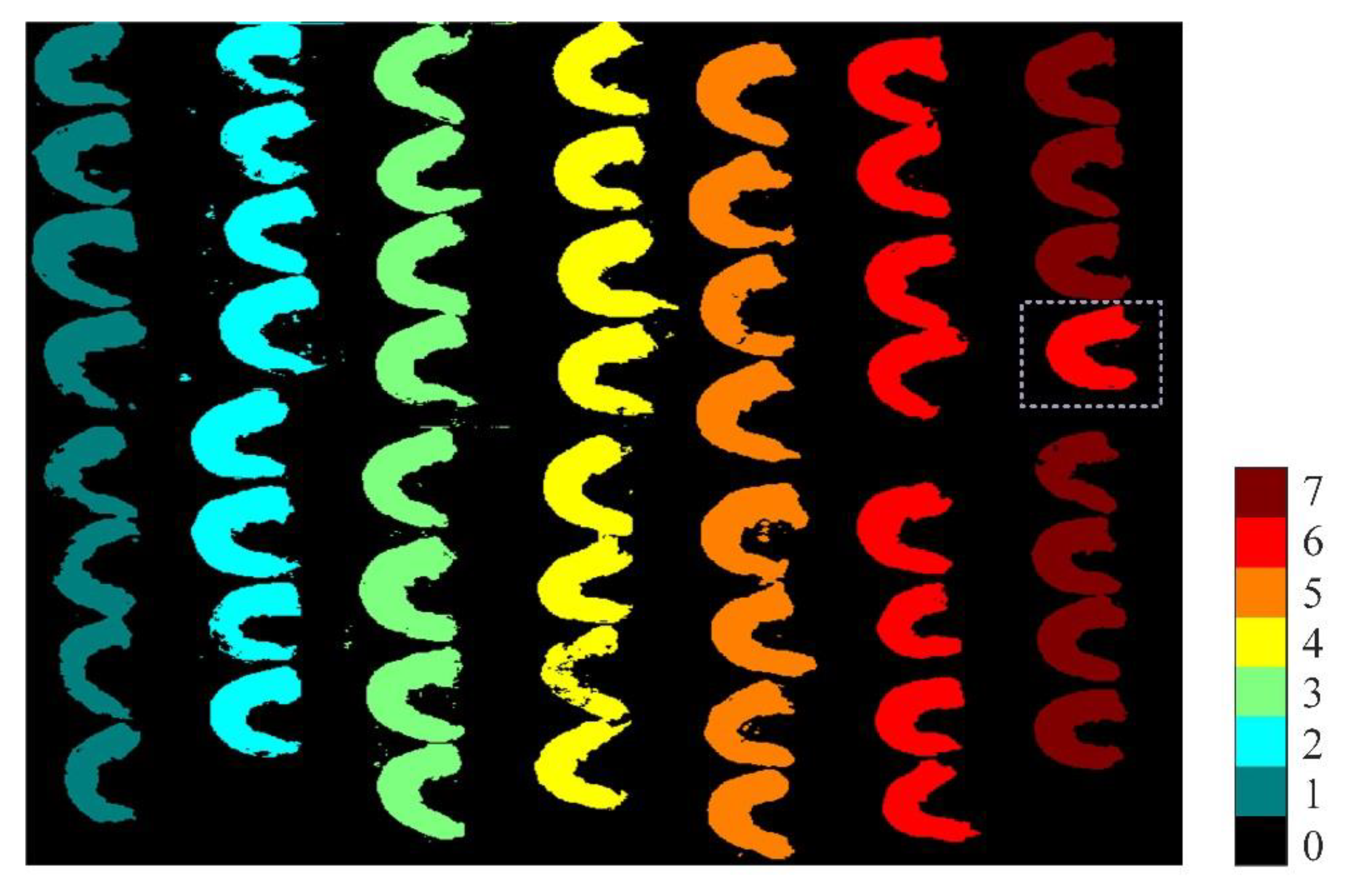
Every day, eight samples were randomly selected from the 7-day experimental samples, and the original hyperspectral images of a total of 56 samples were input into the SNV-CARS-ELM model and visualized by the object-wise method. Figure 9 shows the visual classification of white shrimp for different days of refrigeration, where each category corresponds to a number in the right-hand column, where the background value is 0. It is clear from the figure that the majority of the classification of white shrimp is correct. One white shrimp category on day 7 was misidentified with an aggregate classification accuracy of 97.92% (47/48). Therefore, the model developed in this study is reliable. In addition, the visualized classification diagram can intuitively and accurately estimate the different refrigeration days of white shrimps, which facilitates quick detection and timely elimination of non-fresh white shrimp, thus ensuring their freshness.

4. Conclusions

In this study, the NIR hyperspectral imaging system of 866.4–1701.0nm was chosen to obtain hyperspectral cube data of white shrimps with different refrigeration days. The models were established by combining multivariate methods, and the white shrimps with different refrigeration days were visualized. The main conclusions are as follows:
(1)
The raw spectral data were pre-processed by SG1, MSC, and SNV, after which the corresponding data were entered into PLS-DA, LSSVM, RF, and ELM discriminant models for full wavelength modeling analysis. The results demonstrated that the SNV-processed spectral data had the best performance among the four discriminant models (the accuracy of the prediction set was better than the other two pre-processing methods and the raw spectral data). Therefore, the SNV-processed spectral data were chosen for subsequent characteristic wavelength extraction so as to dimensionally downscale the raw spectra and further improve the model performance.
(2)
The SNV-processed spectral data were extracted by RFA, UVE, and CARS, respectively, and the characteristic wavelengths corresponding to the data were entered into PLS-DA, LSSVM, RF, and ELM discriminant models for modeling and analysis. The comparison with the results of the full wavelength modeling analysis reveals improved modeling results based on characteristic wavelengths, which indicates that the characteristic wavelengths extracted by the three characteristic wavelength extraction algorithms are robust. Additional analyses showed that the combination of CARS and discriminant models had the best performance among the three characteristic wavelength extraction algorithms, while the ELM had the best classification performance among the four discriminant models. Therefore, the SNV-CARS-ELM model was finally chosen as the optimal model.
(3)
To intuitively judge the white shrimps of different refrigeration days, a total of 56 random original hyperspectral images were input into the SNV-CARS-ELM model and visualized by the object-wise method. The classification visualization results showed that only 1 sample out of the total of 48 white shrimp samples was misclassified with an aggregate classification accuracy of 97.92%, which indicates the reliability of the chosen model.
The present results indicate that the combination of NIR hyperspectral imaging technology and multivariate methods is feasible to identify the freshness of white shrimp, which could provide a theoretical foundation for the development of a system for online determination of shrimp freshness by using hyperspectral imaging.

Author Contributions

R.Y. conducted the experiments, analyzed the data, and wrote the paper. Y.C., Y.G., Q.D. and D.L. prepared the experimental materials and analyzed the data. C.L. conceived and designed the experiments. All authors reviewed the manuscript. All authors have read and agreed to the published version of the manuscript.

Funding

This research is supported by China’s national key research and development program (Project No.: 2017YFE0122100).

Acknowledgments

We are deeply grateful to the reviewers and the editors for their valuable comments and suggestions, which improved the technical content and presentation of the paper.

Conflicts of Interest

The authors declare no conflicts of interest.

References

  1. Qiao, X.; Yang, L.; Gao, Q.; Yang, S.; Li, Z.; Xu, J.; Xue, C. Oxidation evaluation of free astaxanthin and astaxanthin esters in Pacific white shrimp during iced storage and frozen storage. J. Sci. Food Agric. 2019, 99, 2226–2235. [Google Scholar] [CrossRef] [PubMed]
  2. Yu, L.; Jiang, Q.; Yu, D.; Xu, Y.; Gao, P.; Xia, W. Quality of giant freshwater prawn (Macrobrachium rosenbergii) during the storage at −18°C as affected by different methods of freezing. Int. J. Food Prop. 2018, 21, 2100–2109. [Google Scholar] [CrossRef] [Green Version]
  3. Pan, C.; Chen, S.; Hao, S.; Yang, X. Effect of low-temperature preservation on quality changes in Pacific white shrimp, Litopenaeus vannamei: A review. J. Sci. Food Agric. 2019, 99, 6121–6128. [Google Scholar] [CrossRef] [PubMed]
  4. Zamora-Méndez, S.; Robles-Romo, A.; Marin-Peralta, E.; Arjona, O.; Apún-Molina, J.P.; Beltrán-Lugo, A.I.; Palacios, E.; Racotta, I.S. Postmortem Metabolic, Physicochemical, and Lipid Composition Changes in Litopenaeus vannamei in Response to Harvest Procedures. J. Aquat. Food Prod. Technol. 2017, 26, 1093–1106. [Google Scholar] [CrossRef]
  5. Le, N.T.; Doan, N.K.; Nguyen Ba, T.; Tran, T.V.T. Towards improved quality benchmarking and shelf life evaluation of black tiger shrimp (Penaeus monodon). Food Chem. 2017, 235, 220–226. [Google Scholar] [CrossRef]
  6. Baptista, R.C.; Horita, C.N.; Sant’Ana, A.S. Natural products with preservative properties for enhancing the microbiological safety and extending the shelf-life of seafood: A review. Food Res. Int. 2020, 127, 108762. [Google Scholar] [CrossRef] [PubMed]
  7. Olatunde, O.O.; Benjakul, S.; Yesilsu, A.F. Antimicrobial Compounds from Crustaceans and Their Applications for Extending Shelf-Life of Marine-Based Foods. Turk. J. Fish. Aquat. Sci. 2020, 20, 629–646. [Google Scholar] [CrossRef]
  8. Ghasemi-Varnamkhasti, M.; Goli, R.; Forina, M.; Mohtasebi, S.S.; Shafiee, S.; Naderi-Boldaji, M. Application of Image Analysis Combined with Computational Expert Approaches for Shrimp Freshness Evaluation. Int. J. Food Prop. 2016, 19, 2202–2222. [Google Scholar] [CrossRef] [Green Version]
  9. Fang, Z.; Zhou, L.; Wang, Y.; Sun, L.; Gooneratne, R. Evaluation the effect of mycotoxins on shrimp (Litopenaeus vannamei) muscle and their limited exposure dose for preserving the shrimp quality. J. Food Process. Preserv. 2019, 43, 1–8. [Google Scholar] [CrossRef]
  10. Khodanazary, A. Freshness assessment of shrimp Metapenaeus affinis by quality index method and estimation of its shelf life. Int. J. Food Prop. 2019, 22, 309–319. [Google Scholar] [CrossRef] [Green Version]
  11. Simoes, J.S.; Mársico, E.T.; De La Torre, C.A.L.; Mano, S.B.; Franco, R.M.; Santos, L.F.L.D.; Conte-Junior, C.A. Nutritional and Sensory Quality of the Freshwater Prawn Macrobrachium rosenbergii and the Influence of Packaging Permeability on its Shelf Life. J. Aquat. Food Prod. Technol. 2019, 28, 703–714. [Google Scholar] [CrossRef]
  12. Thimmappa, M.H.; Manjunatha Reddy, A.; Prabhu, R.M.; Elavarasan, K. Quality Changes in Deep-Sea Shrimp (Aristeus alcocki) During Ice Storage: Biochemical and Organoleptic Changes. Agric. Res. 2019, 8, 497–504. [Google Scholar] [CrossRef]
  13. Feng, C.; Makino, Y.; Oshita, S.; García Martín, J.F. Hyperspectral imaging and multispectral imaging as the novel techniques for detecting defects in raw and processed meat products: Current state-of-the-art research advances. Food Control. 2018, 84, 165–176. [Google Scholar] [CrossRef]
  14. Dai, Q.; Cheng, J.; Sun, D.; Zhu, Z.; Pu, H. Prediction of total volatile basic nitrogen contents using wavelet features from visible/near-infrared hyperspectral images of prawn (Metapenaeus ensis). Food Chem. 2016, 197, 257–265. [Google Scholar] [CrossRef]
  15. Yu, X.; Tang, L.; Wu, X.; Lu, H. Nondestructive Freshness Discriminating of Shrimp Using Visible/Near-Infrared Hyperspectral Imaging Technique and Deep Learning Algorithm. Food Anal. Methods. 2018, 11, 768–780. [Google Scholar] [CrossRef]
  16. Sivertsen, A.H.; Kimiya, T.; Heia, K. Automatic freshness assessment of cod (Gadus morhua) fillets by Vis/Nir spectroscopy. J. Food Eng. 2011, 103, 317–323. [Google Scholar] [CrossRef]
  17. Cheng, J.; Sun, D.; Pu, H.; Chen, X.; Liu, Y.; Zhang, H.; Li, J. Integration of classifiers analysis and hyperspectral imaging for rapid discrimination of fresh from cold-stored and frozen-thawed fish fillets. J. Food Eng. 2015, 161, 33–39. [Google Scholar] [CrossRef]
  18. Reis, M.M.; Van Beers, R.; Al-Sarayreh, M.; Shorten, P.; Yan, W.Q.; Saeys, W.; Klette, R.; Craigie, C. Chemometrics and hyperspectral imaging applied to assessment of chemical, textural and structural characteristics of meat. Meat Sci. 2018, 144, 100–109. [Google Scholar] [CrossRef] [Green Version]
  19. Ndlovu, P.F.; Magwaza, L.S.; Tesfay, S.Z.; Mphahlele, R.R. Rapid visible-near infrared (Vis-NIR) spectroscopic detection and quantification of unripe banana flour adulteration with wheat flour. J. Food Sci. Technol. 2019, 56, 5484–5491. [Google Scholar] [CrossRef]
  20. Yuan, R.; Liu, G.; He, J.; Ma, C.; Cheng, L.; Fan, N.; Ban, J.; Li, Y.; Sun, Y. Determination of metmyoglobin in cooked tan mutton using Vis/NIR hyperspectral imaging system. J. Food Sci. 2020, 85, 1403–1410. [Google Scholar] [CrossRef]
  21. Zhang, L.; Rao, Z.; Ji, H. NIR Hyperspectral Imaging Technology Combined with Multivariate Methods to Study the Residues of Different Concentrations of Omethoate on Wheat Grain Surface. Sensors 2019, 19, 3147. [Google Scholar] [CrossRef] [PubMed] [Green Version]
  22. Li, J.; Zhang, H.; Zhan, B.; Zhang, Y.; Li, R.; Li, J. Nondestructive firmness measurement of the multiple cultivars of pears by Vis-NIR spectroscopy coupled with multivariate calibration analysis and MC-UVE-SPA method. Infrared Phys. Technol. 2020, 104, 103154. [Google Scholar] [CrossRef]
  23. Hong, G.; Abd El-Hamid, H.T. Hyperspectral imaging using multivariate analysis for simulation and prediction of agricultural crops in Ningxia, China. Comput. Electron. Agric. 2020, 172, 105355. [Google Scholar] [CrossRef]
  24. Bai, Z.; Hu, X.; Tian, J.; Chen, P.; Luo, H.; Huang, D. Rapid and nondestructive detection of sorghum adulteration using optimization algorithms and hyperspectral imaging. Food Chem. 2020, 331, 127290. [Google Scholar] [CrossRef] [PubMed]
  25. Wang, C.; Wang, S.; He, X.; Wu, L.; Li, Y.; Guo, J. Combination of spectra and texture data of hyperspectral imaging for prediction and visualization of palmitic acid and oleic acid contents in lamb meat. Meat Sci. 2020, 169, 108194. [Google Scholar] [CrossRef]
  26. Hong, Y.; Chen, S.; Chen, Y.; Linderman, M.; Mouazen, A.M.; Liu, Y.; Guo, L.; Yu, L.; Liu, Y.; Cheng, H.; et al. Comparing laboratory and airborne hyperspectral data for the estimation and mapping of topsoil organic carbon: Feature selection coupled with random forest. Soil Tillage Res. 2020, 199, 104589. [Google Scholar] [CrossRef]
  27. Ahmad, M.; Shabbir, S.; Oliva, D.; Mazzara, M.; Distefano, S. Spatial-prior generalized fuzziness extreme learning machine autoencoder-based active learning for hyperspectral image classification. Optik 2020, 206, 163712. [Google Scholar] [CrossRef]
  28. Yan, L.; Pang, L.; Wang, H.; Xiao, J. Recognition of different Longjing fresh tea varieties using hyperspectral imaging technology and chemometrics. J. Food Process Eng. 2020, 43, e13378. [Google Scholar] [CrossRef]
  29. Yan, Y.; Chen, B.; Zhu, D. Near Infrared Spectroscopy-Principles, Technologies and Application; China Light Industry Press: Beijing, China, 2013; pp. 24–25. [Google Scholar]
  30. Baek, I.; Kusumaningrum, D.; Kandpal, L.; Lohumi, S.; Mo, C.; Kim, M.; Cho, B. Rapid Measurement of Soybean Seed Viability Using Kernel-Based Multispectral Image Analysis. Sensors 2019, 19, 271. [Google Scholar] [CrossRef] [Green Version]
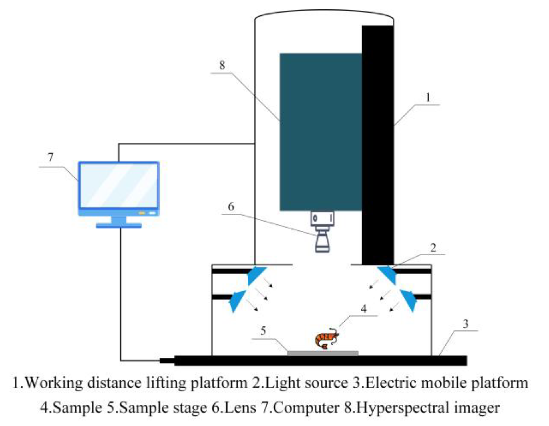
Figure 1. Structure diagram of main components of hyperspectral imaging system.
Applsci 10 05498 g001
Figure 2. Main steps of extracting spectral data, characteristic wavelength, and establishing discrimination model.
Applsci 10 05498 g002
Figure 3. Original spectral curve.
Applsci 10 05498 g003
Figure 4. Average spectral curve.
Applsci 10 05498 g004
Figure 5. Modeling analysis results based on full wavelength.
Applsci 10 05498 g005
Figure 6. Selection probability of each wavelength by utilizing random frog algorithm (RFA).
Applsci 10 05498 g006
Figure 7. Variable stability analysis based on uninformative variables elimination (UVE).
Applsci 10 05498 g007
Figure 8. Process of selecting characteristic wavelengths based on competitive adaptive reweighted sampling (CARS).
Applsci 10 05498 g008
Figure 9. Visualization of White Shrimp on Different Refrigeration Days.
Applsci 10 05498 g009
Table 1. The characteristic wavelengths and the corresponding molecular vibration extracted by random frog algorithm (RFA).
MethodNO.Wavelengths (nm)Molecular Vibration
RFA111078.3Second overtone of C-H + Second overtone of C-C
1132.3, 1175.8, 1209.2, 1212.5, 1222.5, 1262.3Second overtone of C-H
1325.0, 1416.6Second overtone of C-H + First overtone of C-H
1432.8First overtone of N-H
1436.1First overtone of O-H
Table 2. The characteristic wavelengths and the corresponding molecular vibration extracted by uninformative variables elimination (UVE).
MethodNO.Wavelengths (nm)Molecular Vibration
UVE52900.9, 907.8, 928.4, 931.8, 935.3, 938.7, 949.0, 952.4Third overtone of C-H
955.8, 959.3, 993.4, 1000.3, 1007.1Second overtone of O-H
1013.9, 1017.3Second overtone of C-H + Third overtone of C-H
1064.8, 1068.2Second overtone of N-H
1128.9, 1132.3, 1135.6, 1139.0, 1142.3, 1145.7, 1149.0, 1152.4, 1155.7, 1159.1, 1165.8, 1175.8, 1209.2, 1212.5, 1222.5, 1225.8, 1229.2, 1232.5, 1235.8, 1239.1, 1242.5Second overtone of C-H
1249.1, 1255.7, 1259.0, 1269.0, 1275.6, 1298.7, 1351.3, 1387.3, 1390.5Second overtone of C-H + First overtone of C-H
1539.2First overtone of O-H
1609.4, 1634.8, 1644.3, 1679.0First overtone of C-H
Table 3. The characteristic wavelengths and the corresponding molecular vibration extracted by competitive adaptive reweighted sampling (CARS).
MethodNO.Wavelengths (nm)Molecular Vibration
CARS7890.5Second overtone of C-H
1081.7, 1088.5Second overtone of C-H + Second overtone of C-C
1155.7, 1159.1Second overtone of C-H
1351.3, 1357.8Second overtone of C-H + First overtone of C-H
Table 4. Modeling analysis based on characteristic wavelengths.
ModelParameterAccuracy of Calibration Set (CCR/%)Accuracy of Prediction Set (CCR/%)
SNV-RFA-PLS-DA785.0882.86
SNV-UVE-PLS-DA2690.1685.71
SNV-CARS-PLS-DA392.0688.57
SNV-RFA-LSSVM(1, 1)93.6590.48
SNV-UVE-LSSVM(0.6, 7)94.6092.38
SNV-CARS-LSSVM(1.4, 5)94.9293.33
SNV-RFA-RF(550, 14)94.6093.33
SNV-UVE-RF(600, 17)96.8395.24
SNV-CARS-RF(500, 15)98.4197.14
SNV-RFA-ELM7995.5695.24
SNV-UVE-ELM6798.7397.14
SNV-CARS-ELM4299.0598.10
Parameter for partial least squares discrimination analysis (PLS-DA) is number of latent variables (LV), parameters for least squares support vector machine (LSSVM) are penalty coefficient (c) and kernel range (σ), parameters for random forest (RF) are the number of trees (ntree) and the number of features (mtry), and parameter for extreme learning machine (ELM) is the number of hidden layer neurons (L).