Evaluation of Combined Satellite and Radar Data Assimilation with POD-4DEnVar Method on Rainfall Forecast

Abstract

Satellite and radar observations represent two fundamentally different remote sensing observation types, providing independent information for numerical weather prediction (NWP). Because the individual impact on improving forecast has previously been examined, combining these two resources of data potentially enhances the performance of weather forecast. In this study, satellite radiance, radar radial velocity and reflectivity are simultaneously assimilated with the Proper Orthogonal Decomposition (POD)-based ensemble four-dimensional variational (4DVar) assimilation method (referred to as POD-4DEnVar). The impact is evaluated on continuous severe rainfall processes occurred from June to July in 2016 and 2017. Results show that combined assimilation of satellite and radar data with POD-4DEnVar has the potential to improve weather forecast. Averaged over 22 forecasts, RMSEs indicate that though the forecast results are sensitive to different variables, generally the improvement is found in different pressure levels with assimilation. The precipitation skill scores are generally increased when assimilation is carried out. A case study is also examined to figure out the contributions to forecast improvement. Better intensity and distribution of precipitation forecast is found in the accumulated rainfall evolution with POD-4DEnVar assimilation. These improvements are attributed to the local changes in moisture, temperature and wind field. In addition, with radar data assimilation, the initial rainwater and cloud water conditions are changed directly. Both experiments can simulate the strong hydrometeor in the precipitation area, but assimilation spins up faster, strengthening the initial intensity of the heavy rainfall. Generally, the combined assimilation of satellite and radar data results in better rainfall forecast than without data assimilation.

1. Introduction

Accurate initial field, boundary conditions and forecast model play important roles in numerical weather prediction (NWP). With the development of the forecast model, the high quality of the initial field is required. Data assimilation has been proved to be an effective way to provide much more accurate initial field. Currently, variational data assimilation and ensemble Kalman filter (EnKF) are the two widely used methods in data assimilation. For example, a four-dimensional variational (4DVar) method can assimilate observations at multiple times with the constraint of the forecast model [1,2]. However, 4DVar cannot provide evolved, flow-dependent covariance model. Furthermore, the development and maintenance of the tangent linear and adjoint model in 4DVar require a lot of computational resources. In comparison, the background-error covariances in EnKF are estimated from an ensemble forecast, which is flow-dependent [3]. EnKF successfully avoids the development of tangent linear and adjoint model. However, it is limited by the quality of the ensemble forecast. Thus, both methods have advantages and disadvantages. In recent decades, the hybrid data assimilation method combined variational and EnKF is proposed to overcome the shortcomings of their own [4,5,6]. Tian [5,7] proposed a POD-4DEnVar method based on proper orthogonal decomposition (POD) and ensemble forecasting, in which the POD technique is adopted to 4DVar, combining the advantages of variational and EnKF method. The POD-4DEnVar method is evaluated by the Lorenz96 model, observing system simulation experiments (OSSEs), and the shallow water wave equation, outperforming 4DVar and EnKF methods with lower computational costs [7]. Besides, this method has been successfully applied to land data assimilation, showing great potential [8,9].

As two kinds of remote sensing observations, satellite and radar data have been the main resource of data assimilation in NWP. During the last few decades, satellite radiances represent the most numerous and widely available observations in numerical weather prediction system. Satellite observations have better spatiotemporal coverage, especially over ocean area where conventional and radar observations are extremely rare. Thus, the assimilation of satellite data in NWP has been widely used to provide synoptic and mesoscale atmospheric conditions, improving the quality of forecast significantly [10,11,12,13,14,15,16]. Compared with satellite data, radar data has higher a temporal and spatial resolution, which can be used to provide a more accurate analysis of three-dimensional wind field and cloud property. Radar data has been applied to the development of convection and improvement of the short-term forecast. Many studies carried out assimilation experiments on radar radial velocity and reflectivity observations, indicating improving forecasts of severe weather events, such as high winds, heavy rainfall, and tornadoes [17,18,19,20,21,22]. Recently, there are some researches of satellite data or radar data assimilation using POD-3/4DEnVar method. Zhang first assimilated satellite observations from Microwave Humidity Sounder (MWHS) and Microwave Temperature Sounder (MWTS) onboard Fengyun-3A with POD-3/4DEnVar method, showing a positive impact on a heavy rainfall forecast [23,24]. Radar data was first assimilated by Pan with the POD-3DEnVar [25]. It was then developed for POD-4DenVar method to assimilate radar radial velocity and reflectivity with the OSSEs by Zhang et al. [26], showing that POD-4DenVar outperformed the local ensemble transform Kalman filter (LETKF) method. Furthermore, POD-4DenVar assimilation of radar data was demonstrated to improve the precipitation forecast through a case study.

Since assimilating satellite and radar observations separately has led to the improvement of model forecasts, simultaneous assimilation of them has recently received a high degree of attention. Jones et al. [27] assimilated satellite infrared brightness temperature (TB) from Advanced Baseline Imager (ABI) with EnKF method, Doppler radar reflectivity, and radial velocity using OSSEs for a cool-season extratropical cyclone. Results indicated that assimilation improved the analysis of water vapor and cloud hydrometeor. Pan et al. [28] assimilated radar radial velocity and reflectivity together with cloud water path and total precipitation water retrieved from satellite, based on En3DVar method. It shows that simultaneous assimilation outperformed radar data assimilation only, especially in an imperfect storm environment. Using EnKF method, Zhang et al. [29] assimilated both radar data and satellite infrared radiance for a tornadic supercell thunderstorm, revealing that satellite data increased the forecast and warning leading time, and radar data provided the information on three-dimension wind field. Combined assimilation of both data yielded the best forecast. Overall, assimilating both satellite and radar observations makes contributions to the improvement of model forecasts, especially for convective weather. However, many studies in the past focus on the assimilation with traditional methods, such as EnKF. The simultaneous assimilation study of satellite and radar data based on POD-4DEnVar methods is not yet available.

The purpose of this study is to realize the assimilation of satellite radiation, radar radial velocity and reflectivity based on POD-4DEnVar method. Firstly, the assimilation system is designed and established. Then, the performance of the assimilation system is evaluated based on statistical results from two series of continuous rainfall process occurred in 2016 and 2017. The specific contribution to forecast improvement of assimilation is analyzed through a rainstorm case. Finally, the advantages of assimilating satellite and radar data with POD-4DEnVar method are discussed.

2. Assimilation Method and Experiment Configuration

2.1. POD-4DEnVar Algorithm

The POD-4DEnVar method is developed from the traditional 4DVar method. The incremental format of the 4DVar cost function is as follows:

$$J(x^{\prime })=\frac{1}{2}{(x^{\prime })}^T{B}^{-1}(x^{\prime })+\frac{1}{2}{\displaystyle \sum _{t=0}^{s-1}{\left[y_t^{\prime }(x^{\prime })-(y_t^{obs}{)}^{\prime }\right]}^T{R}_t^{-1}\left[y_t^{\prime }(x^{\prime })-(y_t^{obs}{)}^{\prime }\right]},$$

(1)

where $x^{\prime }=x-x_b$ represents the perturbation of the background field $x_b$, $B$ and $R$ are the error covariances of background and observations. s is the total number of observations in the assimilation window. $y_t^{\prime }(x^{\prime })$ is the perturbation of the observations at the analysis time t, and $(y_t^{obs}{)}^{\prime }$ is the observation innovation, which are

$$y_t^{\prime }(x^{\prime })=\left[\begin{array}{l}{y}_1^{\prime }(x^{\prime })\\ y_2^{\prime }(x^{\prime })\\ \dots \\ y_s^{\prime }(x^{\prime })\end{array}\right],$$

(2)

$$y_t^{\prime }(x^{\prime })=y_t^{\prime }(x_b+x^{\prime })-y_t^{\prime }(x_b),\hspace{1em}t=1,2,\dots ,s,$$

(3)

$$(y_t^{obs}{)}^{\prime }=\left[\begin{array}{l}(y_1^{obs}{)}^{\prime }\\ (y_2^{obs}{)}^{\prime }\\ \dots \\ (y_s^{obs}{)}^{\prime }\end{array}\right],$$

(4)

Unlike the traditional 4DVar method, POD-4DEnVar solve the cost function in (1) by constructing ensemble members, which avoids the development of the tangent linear and adjoint model. N ensemble members $(x_1,x_2,\cdots ,x_N)$ are obtained by ensemble forecast, which generate N ensemble perturbations $(x_1^{\prime },x_2^{\prime },\cdots ,x_N^{\prime })$ to the background field $x_b$, where $x_i^{\prime }=x_i-x_b(i=1,2,\cdots ,N)$. Then the ensemble perturbations make up the model perturbations (MPs) matrix $X^p$. In the meantime, N observation perturbations $(y_1^{\prime },y_2^{\prime },\cdots ,y_N^{\prime })$ are constructed by applying the observation operator H in ensemble members and background field $y_t=H_t(M_{1\to t}x)$ ($M_{1\to t}$ is the forecast model), making up the observation perturbation (OPs) matrix $Y^p$.

Since the dimension of the observed variable space is much smaller than that of the model space [6], the POD decomposition is performed on the observation perturbation matrix $Y^p$.

$${(Y^p)}^T(Y^p)=V{\mathsf{\Lambda }}^2{V}^{\mathrm{T}},$$

(5)

Here $V$ and $\mathsf{\Lambda }$ are the decomposed eigenvector and eigenvalue. Then the OPs matrix is transformed as

$$P_y=Y^{p}V,$$

(6)

The POD transformed MPs matrix $P_x$ is defined as

$$P_x=X^{p}V,$$

(7)

The optimal solution $x^{\prime }$ and its corresponding optimal observations perturbation $y^{\prime }$ can be expressed by the linear combinations of the POD-transformed MPs and OPs matrix:

$$x\prime =P_x\beta ,y\prime =P_y\beta ,$$

(8)

Substituting (8) and the ensemble background covariance $B=P_x{P}_x{}^T/(N-1)$ into the incremental format of 4DVar cost function (1)

$$J(\mathsf{\beta })=\frac{1}{2}(N-1)\cdot {\mathsf{\beta }}^T{P}_x^T{\left(P_x^T\right)}^{-1}{\left(P_x\right)}^{-1}{P}_x\mathsf{\beta }+\frac{1}{2}{\left(P_y\mathsf{\beta }-(y_{}^{obs}{)}^{\prime }\right)}^T{R}^{-1}\left(P_y\mathsf{\beta }-(y_{}^{obs}{)}^{\prime }\right)$$

(9)

Finally, the optimal solution $x_{}^{\prime }$ can be expressed as

$$x\prime =P_x{\left[(N-1)I+P_y^T{R}^{-1}{P}_y\right]}^{-1}{P}_y^T{R}^{-1}\left(y^{obs}\right)\prime ,$$

(10)

2.2. Component of the Assimilation System

The POD-4DEnVar assimilation and forecast system mainly consists of three components: Ensemble forecast, assimilation and forecast module, as is shown in Figure 1. The nature of POD-4DEnVar method is constructing flow-dependent background error covariance by making four-dimension ensemble forecast. Thus, the ensemble forecast plays an important role in the implementation of POD-4DenVar, which is essential in improving the assimilation impact. In order to make the ensemble member reveal the real atmosphere, as well as decrease the computational costs, the historical samples are employed to generate the four-dimension ensemble samples [6]. The ensemble forecast is developed with the Weather Research and Forecast (WRF) model. Due to the different temporal and spatial resolution of satellite and radar observations, satellite data is assimilated in the outer domain (D1), and radar data is assimilated in the inner domain (D2). Therefore, nested ensemble samples should be generated by the ensemble forecast.

The second part of the system will assimilate satellite and radar observations separately. According to the POD-4DenVar method, the Ops matrix will be decomposed in D1 and D2. Then the MPs and Ops matrix are transformed by the decomposed eigenvector. The optimal solution can be obtained separately for satellite and radar assimilation. Finally, a deterministic forecast will be made by the WRF model, with the boundary condition updated by satellite and radar assimilation analysis. In the subsequent sections, key points of the main components are described in detail.

2.3. Construction of Four-Dimension Ensemble Samples

The satellite observations are assimilated with a ±3-h assimilation window. Taking 0000 UTC 30 June 2017 as the analysis time, for example, the assimilation window for the satellite is from 2100 UTC 29 June to 0300 UTC 30 June 2017. All observations and ensemble samples are processed and grouped in 7 sub-windows (slot 1 through slot 7), shown in Figure 2. The construction of ensemble samples is shown in Figure 3. Firstly, two predictions (R1 and R2) are made from different sets of initial time (before 6 and 12 h) to 0600 UTC 29 June. Then the two prediction results are used as initial conditions, making two 36-h integrations from 0600 UTC 29 to 1800 UTC 30 June with model output every 1 h. According to the grouped seven sub-windows within the 6-h assimilation window, every ensemble sample consists of seven model output every 1 h. Thus, 62 ensemble samples are obtained through sliding the time point of 1-h model output.

Since the observations of radar are obtained every 6 min, the radar assimilation window is set as 1 h from 0000 UTC 30 June to 0100 UTC 30 June 2017, with the analysis time at the beginning of the time window. All observations and ensemble samples are processed and grouped in 11 sub-windows. Like a satellite, the construction of radar ensemble samples is as follows. Firstly, two predictions (r1 and r2) are made from different initial time (before 8 and 14 h) to 2000 UTC 29 June 2017. After that, r1 and r2 results are used as initial conditions, making two 8-h integrations with the model output every 6 min, which corresponds to the radar scanning frequency. Each ensemble sample should consist of 11 ensemble members, since the model generates output every 6 min during the 1-h time window. Thus, 142 ensemble samples are obtained through slide the time point from 2000 UTC 29 June to 0400 UTC 30 June 2017, which is like satellite ensemble samples.

2.4. Satellite and Radar Data Assimilation Scheme

According to the optimal solution in (10), the construction of MPs matrix and OPs matrix is essential to the implementation of POD-4DEnVar method. For satellite data assimilation, since the satellite-observed brightness temperature (TB) is not model variables, the observation operator is required to calculate TB. Within the WRF Data Assimilation system (WRFDA), the Community Radiative Transfer Model (CRTM) is used as the observation operator [30]. CRTM calculates model-simulated TB from WRF temperature and moisture profiles. In the system, CRTM is run to produce the simulated TB for ensemble members and background field, then making up the OPs matrix.

Like satellite data assimilation, the radar-observed radial velocity and reflectivity are also not model variables. In this case, an observation operator for radar is needed in order to assimilate them directly. The observation operator for radial velocity is

$$V_r=u\frac{x-x_r}{r}+v\frac{y-y_r}{r}+(w-V_{Tm})\frac{z-z_r}{r},$$

(11)

in which, $(u,v,w)$ is the three-dimensional wind field, r is the direction from model grid point $(x,y,z)$ to radar location $(x_r,y_r,z_r)$. $V_{Tm}$ is the terminal velocity of the precipitation, given by Sun and Crook (1997, 1998) [17,18].

$$V_{Tm}=5.40a{q}_r^{0.125},$$

(12)

$$a={\left(\frac{P_0}{\overline{P}}\right)}^{0.4},$$

(13)

where $\overline{P}$ represents the base-state pressure and $P_0$ is the surface pressure.

The observation operator for reflectivity is [19]

$$Z=43.1+17.5\log (\rho q_r),$$

(14)

where $\rho$ is the air density, and $q_r$ is the rainwater mixing ratio. According to the observation operators developed for radar, radial velocity and reflectivity can be calculated from the wind field, rainwater mixing ratio and other model variables, then making up the Ops for radar data assimilation.

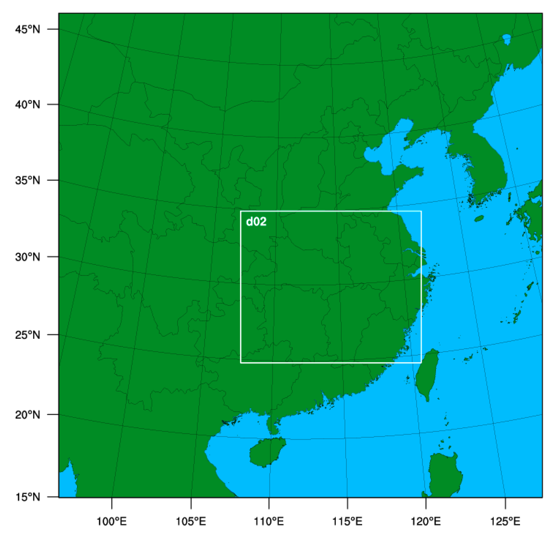
2.5. Experiment Configuration

To investigate the impact of simultaneous assimilating satellite and radar data with POD-4DEnVar method, a series of analysis and forecasts are made from 0000 UTC 27 June 2016 to 0000 UTC 7 July 2016 and 0000 UTC 28 June 2017 to 0000 UTC 8 July 2017, during which obvious summer precipitation in China took place.

Two experiments are conducted in this study. A baseline experiment (CON) is carried out without any assimilation. The second experiment (POD) assimilates satellite radiance and radar radial velocity and reflectivity observations with POD-4DEnVar method, with the analysis time at 0000 UTC for each day. The POD experiment assimilates channel 5–9 (central frequencies from 53.596 to 57.290 GHz, respectively) radiance observations of advanced microwave Sounding Unit-A (AMSU-A) from METOP-2, NOAA-15, NOAA-16, NOAA-18 and NOAA-19. The assimilation time window for the satellite is 6 h, consist of seven sub-windows every 1 h. Before assimilation, satellite observations are thinned to 120 km, after which the quality control procedure is necessary. Doppler radar radial velocity and reflectivity are also assimilated in POD. The assimilation time window of radar is 1 h, with 11 sub-windows every 6 min.

Assimilation is carried out at 0000 UTC each day. The samples are prepared before assimilation, the number of which is 62 for satellite and 142 for radar according to the number of sub-windows. After the data assimilation, 48-h deterministic forecast is run initiated at 0000 UTC each day. The ensemble forecast and final deterministic forecast are made in the WRF model. The WRF model is configured with a two-domain nested grid system, shown in Figure 4. The horizontal resolution of the outer domain is 9 km, with the grid points 400 × 400 for satellite data assimilation. The horizontal resolution of the inner domain is 3 km, with the grid points 400 × 376 for radar data assimilation. Both domains have 35 vertical layers, with the model top at 50 hPa. The boundary conditions are updated every 6 h from the 1 × 1° National Centers for Environmental Prediction (NCEP) Final Operational Model Global Tropospheric Analysis. Overall, 22 analysis and forecast results are obtained finally, which will be used to evaluate the statistical impact of POD-4DEnVar assimilation.

The main physical parameterization schemes in ensemble forecast and deterministic forecast are shown in

Table 1. Physical parameterization schemes.

Microphysics	WSM 6-Class Graupel Scheme
Cumulus parameterization	Kain-Fritsch (new Eta) scheme (none in the inner domain)
Planetary boundary layer	YSU (Yonsei University)
Surface layer	Revised MM5 Monin-Obukhov scheme
Longwave radiation	Rapid Radiative Transfer Model for GCMs
Shortwave radiation	Dudhia scheme

.

3. Results

3.1. Evaluation of the Assimilation System

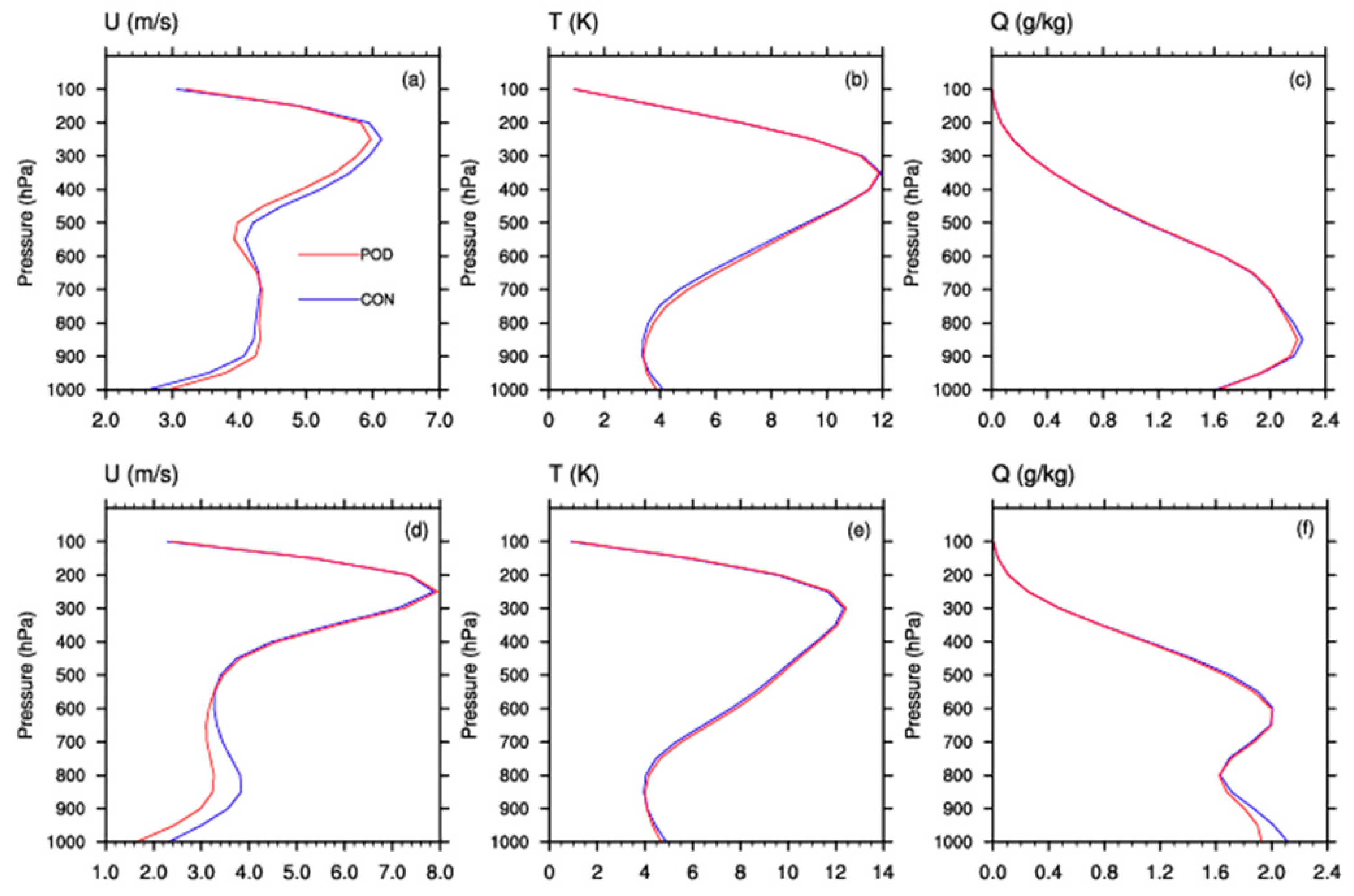
3.1.1. Comparison of Forecast Field

In order to evaluate the performance of the assimilation system, aggregated root-mean-square-error (RMSE) vertical profiles of horizontal wind field, temperature, and water vapor mixing ratio (Qv) forecast at 24-h are shown in Figure 5. The RMSE is calculated within the inner domain, verified against the 0.25 × 0.25° ERA5 reanalysis from the European Centre for Medium-Range Weather Forecasts (ECMWF). The RMSE of 2016 is calculated by averaging the RMSE of 11 24-h forecasts in 2016, and so does 2017. For 2016, POD has its greatest impact on horizontal wind above 600 hPa (Figure 5a). For temperature forecast (Figure 5b), POD is close to CON experiment, with slight improvement near the surface. For water vapor mixing ratio (Figure 5c), the RMSE is slightly decreased in the middle and lower levels. The statistic results from 2017 are shown in Figure 5d–f). Clear reduction of RMSE in POD shows in the middle and lower levels for horizontal wind. Above 500 hPa, POD reveals almost the same profiles with CON. Similar to the 2016 statistic results, POD has little impact on temperature forecast. POD outperforms CON in the water vapor mixing ratio forecast in the lower pressure levels. Overall, though the average RMSE of 24-h forecast is sensitive to different pressure levels of different variables, generally the improvements can be found with assimilation.

Figure 6 shows the average RMSE evolution as the forecast time increases for U and V at 10 m, T and water vapor mixing ratio (Qv) at 2 m. RMSE is averaged for all the 22 forecasts. The RMSE of U and V at 10 m increase with forecast time (Figure 6a,b). The improvements of assimilation appear approximately at 6th hour, after which POD reduces RMSE throughout the remaining forecast period. For T (Figure 6c) and Qv (Figure 6d), POD experiment mainly maintains lower RMSE than CON, though the improvement is smaller than wind field. Overall, POD has a positive impact on the forecast field compared to CON, which indicates the improvement of assimilating satellite and radar data with POD-4DEnVar method.

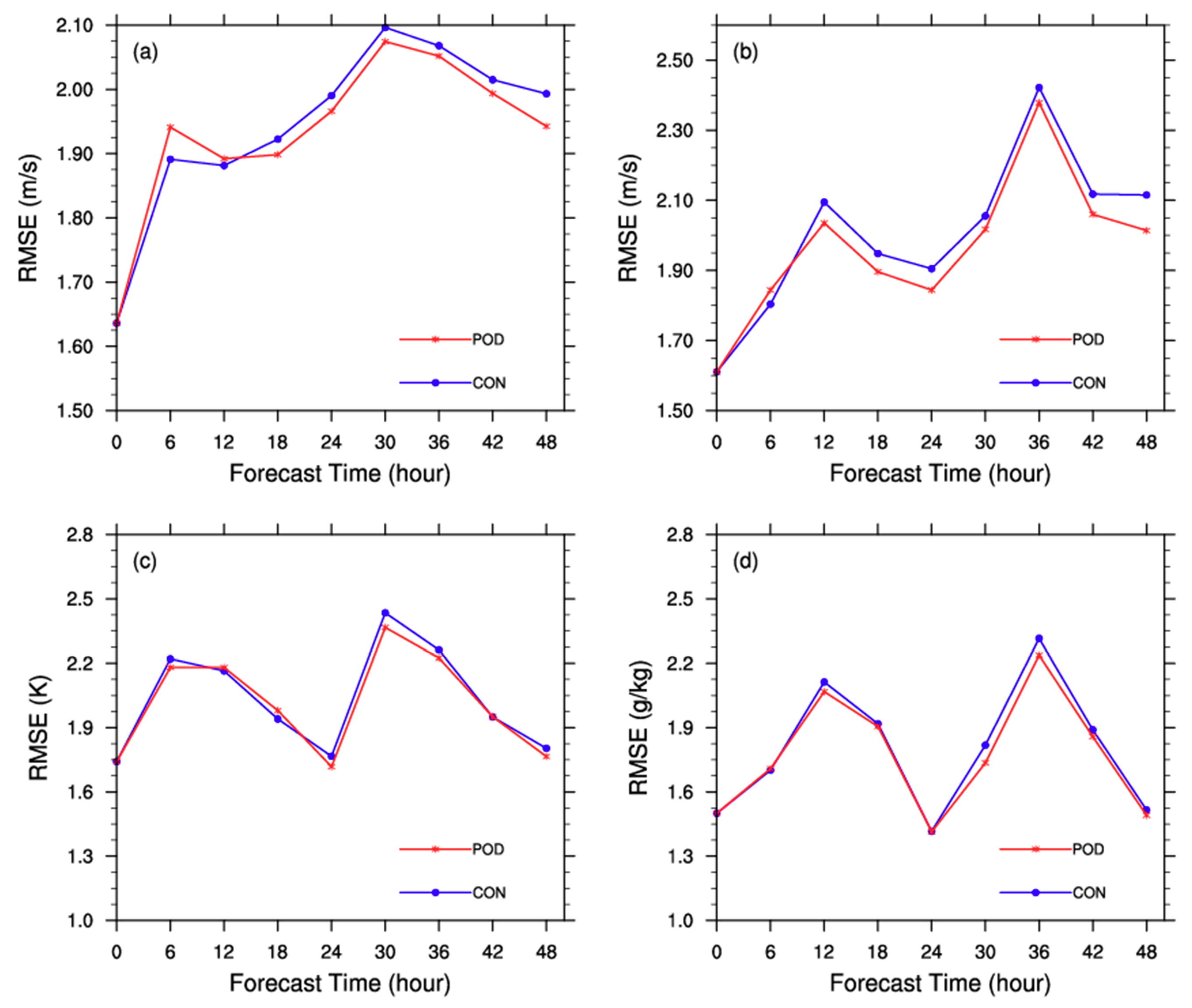
3.1.2. Quantitative Evaluation of Rainfall Forecasts

To quantitatively assess the impact of POD-4DEnVar assimilation on precipitation forecast, the results of 24-h Equitable Threat Score (ETS) from 2016 and 2017 are shown in Figure 7, for five thresholds 0.1 mm, 10 mm, 25 mm, 50 mm and 100 mm per 24 h. The ETS results are aggregated by 11 forecast results per year, compared with the 0.1° × 0.1° precipitation data from the China meteorological data sharing service network (http://data.cma.cn/data/).

For precipitation in 2016 (Figure 7a), the improvements are mainly found in threshold smaller than 50 mm. Compared to CON, POD produces a 2.21% ETS improvement rate for the 0.1 mm precipitation, and 3.25% improvement for 10 mm. Scores of 25 mm in POD is close to CON, with only 0.78% improvement to CON. It shows that weaker precipitation is better represented in 2016 when data assimilation is applied. For heavy rainfall (threshold larger than 50 mm), POD performs worse than CON. For 2017 precipitation (Figure 7b), POD shows comparable or improved ETS for all thresholds. Especially for heavy rainfall in 2017, ETS from POD is improved for 50 mm and 100 mm relative to CON. According to observed precipitation, there has been a heavy rainfall event in Hunan province, China from 29 June 2017 to 1 July 2017 (Figure 8). Results indicate the ability to make a better forecast on heavy rainfall in 2017 when carrying out assimilation. Moreover, relative 0.78% improvement in 0.1 mm, 5.89% in 10 mm and 3.89% in 25 mm are also found in POD relative to CON experiment. Overall, the assimilation of satellite and radar data with POD-4DenVar method show benefits on the rainfall forecast.

3.2. A Rainstorm Forecast Result Analysis

A case study of heavy rainfall from 30 June 2017 to 1 July 2017 is used to understand the impact of satellite and radar data assimilation with POD-4DenVar method. The observed 24-h accumulated precipitation is shown in Figure 8. During that time, heavy rainfall occurred mainly in Hunan Province, China. In the northern-central Hunan, precipitation of most area exceeded 100 mm/24 h, as rainstorm-magnitude. Furthermore, on the northern border between Hunan and Jiangxi Provinces, the amount of precipitation was greater than 200 mm/24 h. The coverage and intensity of the heavy rainfall in Hunan far surpassed historical levels, causing severe economic and humanitarian losses of Hunan Province.

3.2.1. Accumulated Rainfall Evolution

In order to compare the performance of different experiments, the accumulated rainfall evolution is displayed in Figure 9. Precipitation is accumulated for 3, 6, 12, and 24 h from the first row to the fourth row, initialized at 0000 UTC 30 June 2017. The left column in Figure 9 is the observed precipitation from the Climate Prediction Center morphing method (CMORPH) products [31], the middle column is the simulated precipitation in CON, and the right column is for POD. The observed precipitation of 3-h accumulation (Figure 9a) is mainly in northern and central Hunan Province, and the border between Jiangxi and Hubei. There are two precipitation cores with the amount of 30 mm. The precipitation in CON also has two cores, but the left one is more to the west than the observation, and the right one is more to the northeast. Furthermore, the amount of the precipitation core in CON is 20 mm, clearly weaker than the observations. Including satellite and radar data, POD obviously captures the precipitation on the border between Jiangxi and Hubei. POD strengths the intensity of rainfall compared to CON, but overpredicts the amount of 3-h accumulated precipitation by 40 mm.

For 6-h forecast, a clear northeast to southwest zone precipitation area is observed in the northeastern Hunan and northwestern Jiangxi Provinces (Figure 9d), with a maximum precipitation of 50 mm. The distribution of rainfall in CON (Figure 9e) is on the west of observations, with the location of precipitation cores mismatching the observations. One core area is in the central of Hunan, and another is on the border between Hubei and Jiangsu for CON. POD (Figure 9f) clearly improves the location of precipitation forecast, such as the rainfall in the northeastern Hunan and northwestern Jiangxi. In addition, the spatial distribution of precipitation in POD better agrees with observations compared with CON.

The location of 12-h accumulated rainfall (Figure 9g) is similar to 6-h accumulated, but with larger coverage area, showing a precipitation core area in northeastern Hunan with the amount of 80 mm. In comparison, POD improves the intensity and location of precipitation forecast in Hunan and Jiangxi Province. Figure 9j–l shows the 24-h accumulated rainfall, with a larger area and stronger intensity in Hunan, Jiangxi, and Hubei. The maximum precipitation exceeds 100 mm. Without assimilation, CON underestimates the coverage of rainfall, with the precipitation core only in Hunan Province. However, POD is of better agreement with observation in the intensity, as well as the shape and location of the precipitation.

In order to evaluate the precipitation results objectively, the Structure, Amplitude and Location (SAL) method is applied [32]. The forecast results with smaller absolute value of S, A and L are better. Figure 10 shows the SAL evaluation scores of 24-h accumulated precipitation at different thresholds. For the threshold >0 mm, the S value in POD is close to CON, slightly smaller than CON. The location forecast is similar to structure, in which POD is slightly smaller than CON. For intensity evaluation, A > 0 means that forecast results are stronger than the observations, A < 0 means the contrary. For 0 mm threshold, POD yields stronger precipitation than the observations, while CON shows a weaker forecast. However, the precipitation intensity forecast is clearly improved, since POD has a smaller absolute value. For the precipitation threshold 50 mm and 100 mm, the structure of the precipitation forecast is significantly improved with assimilation. Similarly, obvious smaller values are found for A and L in POD, which means better intensity and location forecast with satellite and radar data assimilated.

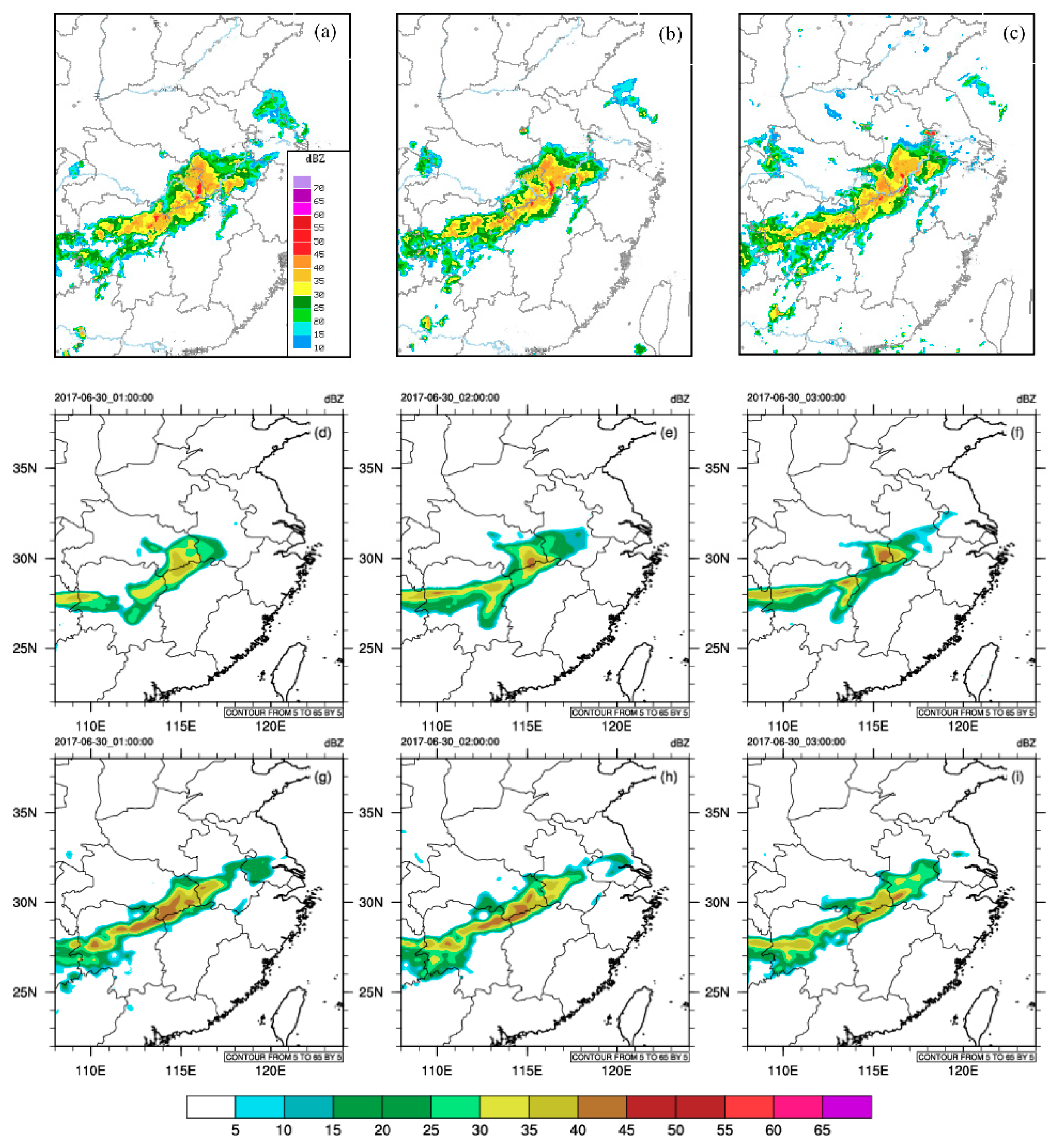
3.2.2. Radar Reflectivity Simulation

The radar reflectivity can be used to reveal the development of convection and hydrometeor, which is important for rainfall development. Figure 11 shows the observed radar reflectivity from 0100 UTC to 0300 UTC 30 June, and simulated reflectivity at a corresponding time from CON and POD experiment. The observed radar reflectivity comes from the radar map of China meteorological data sharing service network (http://data.cma.cn/data/online/t/4). According to the observed radar reflectivity (Figure 11a–c), clear radar echo is found from southwest to northeast in the precipitation area The reflectivity of 40 dBZ (with a maximum of 45 dBZ) appears in the border among Hunan, Jiangxi and Hubei Provinces, indicating strong convection.

At 0100 UTC, the reflectivity (>10 dBZ) from CON (Figure 11d) is mainly located in the border among Hunan, Jiangxi and Hubei province, with the maximum reflectivity of about 35 dBZ. Obviously, the reflectivity in CON is weaker than the observation. In comparison, stronger convections are found in POD (Figure 11g). The coverage of reflectivity in POD is better consistent with observation, with a maximum of 40 dBZ. However, the area of 40 dBZ is slightly larger than the observations. It is inferred that at the beginning of forecast, the convection is slightly overpredicted, which is consistent with the overestimated rainfall in Figure 9. At 0200 UTC, the reflectivity in CON (Figure 11e) is strengthened a little, with a maximum up to 40 dBZ. However, it remains a weaker intensity and smaller area than the observations. For POD (Figure 11h), the area of 40 dBZ decreases compared to the first hour of the forecast. Thus, since POD overestimates the intensity of convention at the beginning of the forecast time, it adjusts itself to agree with observations. However, a relative stronger reflectivity can be found compared to CON. In the border among Hunan, Jiangxi and Hubei, where the main precipitation took place, POD yields about 40 dBZ, while 30–35 dBZ in CON. Similar results appear at 0300 UTC, in which reflectivity in POD shows better agreement with observation.

Overall, the comparison of simulated reflectivity with observation provides more insight into the differences with and without assimilations. POD better capture the convection in the heavy rainfall area. Thus, assimilating satellite and radar data is able to strengthen the development of convection, improving the forecast of heavy rainfall.

3.2.3. Effects of Assimilation on Initial Field

In order to figure out the contributions to the improved precipitation forecasts on how the assimilation changes the initial conditions, the analysis increments (analysis minus background) at 0000 UTC 30 June 2017 are compared from Figure 12, Figure 13 and Figure 14.

Figure 12a shows the overlaid of water vapor mixing ratio increments and analysis wind field. Obvious southwesterly flow is found on the south of the precipitation area, advecting warm and moist air from the south. In the main precipitation area (Hunan Province), POD produces positive increments at 700 hPa, improving the water vapor mixing ratio. To better understand the vertical structure of water vapor changes, the cross-section is made along the red line in Figure 12a, which is shown in Figure 12b. Large positive increments appear under 500 hPa, revealing that assimilating satellite data increase water vapor dramatically in the mid-lower level. Similarly, the temperature increments are shown in Figure 12c–d. Negative increments are found mainly at 700 hPa, indicating that assimilation has a cooling effect in the low level of precipitation area. However, the temperature increase is found in the upper level when cross-section is made (Figure 12d). It can be inferred that strong convection develops in the heavy rainfall event, with convective condensation latent heat in the upper level of precipitation area.

Figure 13 shows the increments of vertical velocity at 500 hPa and associated cross-sections of the wind field. From Figure 13a, assimilation strengthens the updraft in the precipitation area. Clearly, southern wind increments appear in the same area, promoting the transportation of warm and wet air from the south of the rainfall area. Figure 13b displays the wind increments and relative humidity analysis, in which a large area of near-saturation humidity covering the main precipitation area, with the top at almost 300 hPa. In addition, assimilation clearly exhibits a strong and deep updraft within the high humidity area. The above results suggest that the combined assimilation of satellite and radar data changes the dynamical (wind) and thermodynamical (temperature and humidity) features which are important for convection development.

Hydrometeor plays an important role in the development of heavy rainfall. From the observation operation in (14), the rainwater mixing ratio q_r clearly affects the direct assimilation of radar data. The distribution of rainwater mixing ratio increments of radar data assimilation is analyzed in Figure 14. Positive increments are clearly found at 850 hPa (Figure 14a). Same results appear in the cross-section along the red line in Figure 14a, in which rainwater mixing ratio is mainly enhanced in the precipitation area from surface to almost 500 hPa. As the hydrometeor, the improvement of rainwater mixing ratio directly strengthens the intensity of heavy rainfall in POD.

Since the initial rainwater has been improved in POD, the vertical structure of hydrometeors as the forecast time leads is showed to exam the continued effect of assimilation. The pressure-time cross-sections are presented for rainwater mixing ratio and cloud water mixing ratio in the different experiments. For rainwater (Figure 15a,b), it is mainly located below 600 hPa. Rainwater appears clearly at about 4 h in CON (Figure 15a), and reach its first maximum magnitude at almost 7 h. In comparison, POD (Figure 15b) generates rainwater at the beginning of forecast because rainwater mixing ratio is directly changed during the assimilation. Three hours later, rainwater reaches its first maximum magnitude for the 8 h forecast. After 12 h forecast, there is no obvious difference between CON and POD. Cloud water mixing ratio (Figure 15c,d) is found at around 600 hPa, which is clearly higher than rainwater. Similarly, relative strong cloud water is found after 6 h forecast in CON (Figure 15c). However, the intensity of cloud water in POD (Figure 15d) is maintained because the forecast begins, starting to decrease in 7 h later. After 16 h forecast, the intensity in CON is close to POD, but still maintains a weaker in intensity compared to POD. Therefore, both experiments can simulate the concentration of hydrometeors, but POD spinning up faster with stronger intensity compared to CON.

4. Discussion

Satellite and radar observations represent the main remote sensing data which can be assimilated into NWP. Many studies analyzed the impacts of assimilating these data, and improvements of forecasts were found [15,16,19,20,33,34,35,36]. A previous study has concentrated on the assimilation with traditional methods, such as 3/4DVAR and EnKF [27,28,29]. This study first simultaneously assimilates satellite and radar data with the POD-4DEnVar method, which combines the advantages of variational and ensemble Kalman filter assimilation methods [5,7]. For example, 4DVAR can assimilate observations at multiple times, but with the static background error variance and lots of computational resources. EnKF can provide flow-dependent background error variance and require less work on coding, maintenance and development of an adjoint model [26], but limited by the quality of the ensemble forecast [2]. Thus, this study utilizes the POD-4DEnVar method to assimilate both satellite and radar data.

The final optimal solution of POD-4DEnVar assimilation method Equation (10) shows that the analysis can be represented by model perturbation $P_x$, observation perturbation matrix $P_y$, the error covariances of observations $R$ and the observation innovation $(y^{obs})\prime$. Thus, the adjoint model of traditional 4DVAR is no longer needed [5]. The ensemble of historical samples is used to construct the perturbation matrix, which is much more economical. The avoid of the adjoint model and choice of historical samples make POD-4DEnVar assimilation much cheaper to run, which is better to be applied in higher-resolution NWP [37]. Furthermore, the B matrix in POD-4DEnVar method is constructed by ensemble forecasts, which is flow-dependent in comparison with the traditional static background error variance [38,39]. The increments in Section 3.2.3 well display the flow-dependent pattern in POD-4DEnVar method. Apparent local increments of wind, temperature and moisture are found in the precipitation area, indicating that POD-4DEnVar assimilation can spread observation information spatially according to the current circulation pattern. The flow-dependent error structure is important for rapidly evolving synoptic systems [40].

In order to make an accurate forecast on precipitation, the accuracy of initial hydrometeor is important [27]. Increment results show that assimilating satellite and radar data with POD-4DEnVar method can improve the initial analysis of hydrometeors for better heavy rainfall forecast (Figure 14 and Figure 15). As is known, the WRF model needs a spin-up time to produce hydrometeor for rainfall forecast, which downgrades the short-term rainfall forecast. Even if the traditional variational assimilation method is applied (e.g., 3DVAR or 4DVAR), the initial field of hydrometeor cannot be changed. Cloud and precipitation processes have a flow-dependent and nonlinear characteristic, but variational assimilation method requires a tangent linear model and its adjoint for nonlinear moist physics parameterization [41], which is not required in POD-4DEnVar method. In addition, POD-4DEnVar can construct flow-dependent background error variance, which can better represent cloud and precipitation process than static background error in the traditional variational analysis [42]. Therefore, hydrometeor can be directly included in the control variables of POD-4DEnVar method. The change in the initial field of hydrometeor can decrease the spin-up time. From the results of hydrometeor simulation, both the experiments can simulate the concentration of hydrometeors. However, CON produces hydrometeor after about 6 h, and POD produces hydrometeor as soon as the forecast begins (Figure 15). The faster spin-up for hydrometeors in POD covers the shortage of traditional variational assimilation method, which is beneficial to short-term forecast, especially less than 6 h. Besides, since POD-4DEnVar method adopts the variational framework, the dynamic constraint and existing capability of variational assimilation can be added in POD-4DEnVar [43,44,45]. In all, POD-4DEnVar combines the advantages of traditional variational assimilation method and EnKF.

Table 2. Comparison of variational data assimilation, ensemble Kalman filter (EnKF), and POD-4DenVar methods.

Advantages	Variational Data Assimilation (3/4DVAR)	EnKF	POD-4DenVar
Benefit from the use of Flow-dependent B		√	√
Better localization for satellite and radar observations [44]	√		√
Easiness to add the dynamic constraint of variation [46]	√		√
No need for linearized models [37]		√	√
More use of existing capability in VAR	√		√

summarizes the difference of variational data assimilation, EnKF and POD-4DEnVar method based on literature [37,43,44,45] and this paper.

Using POD-4DEnVar assimilation method, previous researchers studied the impact of assimilating satellite and radar data individually [24,26]. In this study, simultaneous satellite and radar data assimilation is performed. Compared to individual assimilation, assimilating two kinds of data provide both information on satellite and radar at the same time. Satellite radiance represents the most numerous and widely available observations and provide information where other observations are not present [27]. Radar observations have much higher-resolution, which is useful for local convective weather system [47]. Increment results show that assimilating both observations can change the large-scale and local initial field. Temperature and moisture are changed almost all over the study domain, while wind field and hydrometeor are only changed in the precipitation area. Similar to results from Sun et al. [48], who assimilated two kinds of observations results in the reasonable analysis of wind, temperature and moisture field, improving the rainstorm forecast. In addition, Zhang et al. [24] found that the benefits of satellite assimilation show in temperature, moisture and wind field, without rainwater included in the control variables. In this study, due to the relationship between radar reflectivity and rainwater Equation (14), rainwater in included in the control variables when assimilating both satellite and radar data. Thus, the increase of initial rainwater help improves rainfall forecast especially, compared to assimilating satellite radiance only. When only assimilating radar data with POD-4DEnVar method, Zhang et al. [26] found that initial rainwater is also changed. However, with the satellite data included in this study, the change on initial hydrometeor (Figure 14) is obviously more widely distributed than Zhang et al. (Figure 10 in [26]). Therefore, assimilating both satellite and radar data with POD-4DEnVar method provides better initial analysis and forecast for heavy rainfall. Furthermore, previous assimilation with POD-4DEnVar method focus on just one case study. Zhang et al. [24] investigated the impacts of POD-4DEnVar assimilating satellite radiance on a heavy rainfall on 29 June 2009. Zhang et al. [26] assimilated radar data with POD-4DEnVar method for heavy rainfall on 08 July 2010. In this study, instead of single analysis and forecast for one case, the performance of the POD-4DEnVar assimilation system is evaluated through two 11-day continuous analysis and forecast in 2016 and 2017, during which obvious summer precipitation took place. The RMSE and precipitation score results are averaged over all the analysis and forecasts during that time. Thus, statistical evaluation on the system is much more valid than just single analysis and forecast for the case study [49].

In all, assimilating satellite and radar data with POD-4DEnVar method shows improvements when making a forecast on heavy rainfall. On the one hand, the flow-dependent increments are produced in the precipitation area according to the current circulation pattern. The better precipitation forecast in POD is attributed to the local change of dynamical and thermodynamic field. On the other hand, assimilation decreases the spin-up time for hydrometeor, which is important for the development of short-term heavy rainfall. Since the precipitation forecast is weaker than the observations in CON, assimilation help strengthens the precipitation, resulting in better forecast performance. Although this study shows encouraging results of simultaneously assimilating satellite and radar data with POD-4DEnVar method, further work is still needed. Firstly, results from the evaluation of the assimilation system show that the benefits of assimilation are still not guaranteed all the time. Thus, more testing and additional cases are required to further evaluate the performance of the system. Secondly, satellite data has been assimilated in all-sky conditions [50,51,52], which is our further goal to assimilate satellite data in all-sky conditions with POD-4DEnVar method. In addition, more efforts are needed to optimize the system in order to be applied in the daily weather forecast.

5. Conclusions

This study firstly establishes the assimilation system of both satellite and radar data based on POD-4DEnVar method, instead of assimilating them separately. The performance of the system is investigated on continuous summer rainfall, which occurred from June to July in 2016 and 2017. The RMSE against ERA-5 reanalysis shows that assimilation with POD-4DEnVar has a neutral or positive impact on the reduction of RMSE from CON. Quantitative verification using ETS indicate that although the benefits of assimilation are not universal guaranteed, the potential of POD-4DEnVar assimilation can still be found. Particularly in 2017, the increase of ETS on heavy rain shows the ability to make short-term heavy rainfall forecast.

The rainstorm on 30 June 2017 help better understand the contribution of assimilating satellite and radar data. Results of simulated reflectivity show that POD yields stronger development of convection than CON, which can also be supported by the precipitation forecast and agree more with observations. The increments on the initial field are also discussed in this paper, revealing that moisture, temperature and wind field in the precipitation area are changed at the initial time with assimilation. The increase of moisture over the precipitation area promotes the water vapor content. Positive increments of temperature increase the convective condensation latent heat. The strengthen of horizontal wind convergence, and vertical velocity enhances the development of convection. In addition, POD strengthens the hydrometeor intensity since the forecast begins. All the contributions prove that POD-4DEnVar assimilation of satellite and radar data has the ability to improve the performance of NWP, which can be further applied in the operational weather forecast.

References

1. Courtier, P.; Thepaut, J.N.; Hollingsworth, A. A strategy for operational implementation of 4DVar using an incremental approach. Q. J. R. Meteorol. Soc. 1994, 120, 1367–1387. [Google Scholar] [CrossRef]
2. Lorenc, A.C. The potential of the ensemble Kalman filter for NWP—A comparison with 4D-VAR. Q. J. R. Meteorol. Soc. 2003, 129, 3183–3203. [Google Scholar] [CrossRef]
3. Zhang, F.; Weng, Y.; Sippel, J.A.; Meng, Z.; Bishop, C.H. Cloud-resolving hurricane initialization and prediction through assimilation of Doppler radar observations with an ensemble Kalman filter. Mon. Weather Rev. 2009, 137, 2105–2125. [Google Scholar] [CrossRef] [Green Version]
4. Qiu, C.; Chou, J. Four-dimensional data assimilation method based on SVD: Theoretical aspect. Theor. Appl. Climatol. 2006, 83, 51–57. [Google Scholar] [CrossRef]
5. Tian, X.; Xie, Z.; Dai, A. An ensemble-based explicit four-dimensional variational assimilation method. J. Geophys. Res. Atmos. 2008, 113. [Google Scholar] [CrossRef]
6. Wang, B.; Liu, J.; Wang, S.; Cheng, W.; Juan, L.; Liu, C.; Xiao, Q.; Kuo, Y.H. An economical approach to four-dimensional variational data assimilation. Adv. Atmos. Sci. 2010, 27, 715–727. [Google Scholar] [CrossRef] [Green Version]
7. Tian, X.; Xie, Z.; Sun, Q. A POD-based ensemble four-dimensional variational assimilation. Tellus Ser. A Dyn. Meteorol. Oceanol. 2011, 63, 805–816. [Google Scholar] [CrossRef]
8. Tian, X.; Xie, Z.; Dai, A.; Shi, C.; Jia, B.; Chen, F.; Yang, K. A dual-pass variational data assimilation framework for estimating soil moisture profiles from AMSR-E microwave brightness temperature. J. Geophys. Res. Atmos. 2009, 114, D16102. [Google Scholar] [CrossRef] [Green Version]
9. Tian, X.; Xie, Z.; Dai, A.; Jia, B.; Shi, C. A microwave land data assimilation system: Scheme and preliminary evaluation over China. J. Geophys. Res. Atmos. 2010, 115, D21113. [Google Scholar] [CrossRef]
10. Houtekamer, P.L.; Mitchell, H.L.; Pellerin, G.; Buehner, M.; Charron, M.; Spacek, L.; Hansen, B. Atmospheric data assimilation with an ensemble Kalman filter: Results with real observations. Mon. Weather Rev. 2005, 133, 604–620. [Google Scholar] [CrossRef] [Green Version]
11. Chen, Y.; Snyder, C. Assimilating vortex position with an ensemble Kalman filter. Mon. Weather Rev. 2007, 135, 1828–1845. [Google Scholar] [CrossRef] [Green Version]
12. Chen, S.H.; Vandenberghe, F.; Petty, G.W.; Bresch, J.F. Application of SSM/I satellite data to a hurricane simulation. Q. J. R. Meteorol. Soc. 2010, 130, 801–825. [Google Scholar] [CrossRef] [Green Version]
13. Buehner, M.; Houtekamer, P.L.; Charette, C.; Mitchell, H.L.; He, B. Intercomparison of variational data assimilation and the ensemble Kalman filter for global deterministic NWP. Part II: One-month experiments with real observations. Mon. Weather Rev. 2010, 138, 1567–1586. [Google Scholar] [CrossRef]
14. Hamill, T.M.; Whitaker, J.S.; Fiorino, M.; Benjamin, S.G. Global ensemble predictions of 2009’s tropical cyclones initialized with an ensemble Kalman filter. Mon. Weather Rev. 2011, 139, 668–688. [Google Scholar] [CrossRef] [Green Version]
15. Liu, Z.; Schwartz, C.S.; Snyder, C.; Ha, S.Y. Impact of assimilating AMSU-A radiances on forecasts of 2008 Atlantic tropical cyclones initialized with a limited-area ensemble Kalman filter. Mon. Weather Rev. 2012, 140, 4017–4034. [Google Scholar] [CrossRef] [Green Version]
16. Zou, X.; Qin, Z.; Weng, F. Improved quantitative precipitation forecasts by MHS radiance data assimilation with a newly added cloud detection algorithm. Mon. Weather Rev. 2013, 141, 3203–3221. [Google Scholar] [CrossRef]
17. Sun, J.; Crook, N.A. Dynamical and microphysical retrieval from Doppler radar observations using a cloud model and its adjoint: Part I. Model development and simulated data experiments. J. Atmos. Sci. 1997, 54, 1642–1661. [Google Scholar] [CrossRef]
18. Sun, J.; Crook, N.A. Dynamical and microphysical retrieval from Doppler radar observations using a cloud model and its adjoint: Part II. Retrieval experiments of an observed Florida convective storm. J. Atmos. Sci. 1998, 55, 835–852. [Google Scholar] [CrossRef]
19. Gao, J.; Xue, M.; Brewster, K.; Droegemeier, K.K. Droegemeier. A three-dimensional variational data assimilation method with recursive filter for single-Doppler radar. J. Atmos. Ocean. Technol. 2004, 21, 457–469. [Google Scholar] [CrossRef]
20. Aksoy, A.; Dowell, D.C.; Snyder, C. A multicase comparative assessment of the ensemble Kalman Filter for assimilation of radar observations. Part I: Storm-scale analyses. Mon. Weather Rev. 2009, 137, 1805–1824. [Google Scholar] [CrossRef] [Green Version]
21. Gao, J.; Stensrud, D.J. Assimilation of reflectivity data in a convective-scale, cycled 3DVAR framework with hydrometeor classification. J. Atmos. Sci. 2012, 69, 1054–1065. [Google Scholar] [CrossRef]
22. Wang, H.; Sun, J.; Zhang, X.; Huang, X.; Auligne’, T. Radar data assimilation with WRF 4D-Var. Part I: System development and preliminary testing. Mon. Weather Rev. 2013, 141, 2224–2244. [Google Scholar] [CrossRef]
23. Zhang, M.; Zhang, L.; Zhang, B.; Guan, J.; You, W. Assimilation of MWHS and MWTS radiance data from the FY-3A satellite with the POD-3DEnVar method for forecasting heavy rainfall. Atmos. Res. 2018, 219, 95–105. [Google Scholar] [CrossRef]
24. Zhang, M.; Zhang, L.; Zhang, B. FY-3A Microwave Data Assimilation Based on the POD-4DEnVar Method. Atmosphere 2019, 9, 189. [Google Scholar] [CrossRef] [Green Version]
25. Pan, X.; Tian, X.; Li, X.; Xie, Z.; Shao, A.; Lu, C. Assimilating Doppler radar radial velocity and reflectivity observations in the weather research and forecasting model by a proper orthogonal decomposition based ensemble three-dimensional variational assimilation method. J. Geophys. Res. Atmos. 2012, 117. [Google Scholar] [CrossRef] [Green Version]
26. Zhang, B.; Tian, X.; Sun, J.; Chen, F.; Zhang, Y.; Zhang, L.; Fu, S. PODEn4DVar-based radar data assimilation scheme: Formulation and preliminary results from real-data experiments with Advanced Research WRF (ARW). Tellus Ser. A Dyn. Meteorol. Oceanol. 2015, 67, 26045. [Google Scholar] [CrossRef] [Green Version]
27. Jones, T.A.; Otkin, J.A.; Stensrud, D.J.; Knopfmeier, K. Assimilation of satellite infrared radiances and Doppler radar observations during a cool season observing system simulation experiment. Mon. Weather Rev. 2013, 141, 3273–3299. [Google Scholar] [CrossRef]
28. Pan, S.; Gao, J.; Stensrud, D.J.; Wang, X.; Jones, T.A. Assimilation of Radar Radial Velocity and Reflectivity, Satellite Cloud Water Path, and Total Precipitable Water for Convective-Scale NWP in OSSEs. J. Atmos. Ocean. Technol. 2018, 35, 60–89. [Google Scholar] [CrossRef]
29. Zhang, Y.; Stensrud, D.J.; Zhang, F. Simultaneous Assimilation of Radar and All-Sky Satellite Infrared Radiance Observations for Convection-Allowing Ensemble Analysis and Prediction of Severe Thunderstorms. Mon. Weather Rev. 2019, 147, 4389–4409. [Google Scholar] [CrossRef]
30. Han, Y.; van Delst, P.; Liu, Q.; Weng, F.; Yan, B.; Han, Y. JCSDA Community radiative Transfer Model (CRTM)-Version 1. NOAA Tech. Rep. NESDIS. 2006, 122, 33. [Google Scholar]
31. Joyce, R.J.; Janowiak, J.E.; Arkin, P.A.; Xie, P. CMORPH: A Method that Produces Global Precipitation Estimates from Passive Microwave and Infrared Data at High Spatial and Temporal Resolution. J. Hydrometeor. 2004, 5, 487–503. [Google Scholar] [CrossRef]
32. Wernli, H.; Paulat, M.; Hagen, M.; Frei, C. SAL—A Novel Quality Measure for the Verification of Quantitative Precipitation Forecasts. Mon. Weather Rev. 2008, 136, 4470–4487. [Google Scholar] [CrossRef] [Green Version]
33. Wang, Y.; Chen, Y.; Min, J. Impact of Assimilating China Precipitation Analysis Data Merging with Remote Sensing Products Using the 4DVar Method on the Prediction of Heavy Rainfall. Remote Sens. 2019, 11, 973. [Google Scholar] [CrossRef] [Green Version]
34. Ban, J.; Liu, Z.; Zhang, X.; Huang, X.; Wang, H. Precipitation data assimilation in WRFDA 4D-Var: Implementation and application to convection-permitting forecasts over United States. Tellus Ser. A Dyn. Meteorol. Oceanol. 2017, 69, 1368310. [Google Scholar] [CrossRef] [Green Version]
35. Xie, Y.; Shi, J.; Fan, S.; Chen, M.; Dou, Y.; Ji, D. Impact of Radiance Data Assimilation on the Prediction of Heavy Rainfall in RMAPS: A Case Study. Remote Sens. 2018, 10, 1380. [Google Scholar] [CrossRef] [Green Version]
36. Lee, J.W.; Min, K.H.; Lee, Y.H.; Lee, G. X-Net-Based Radar Data Assimilation Study over the Seoul Metropolitan Area. Remote Sens. 2020, 12, 893. [Google Scholar] [CrossRef] [Green Version]
37. Bannister, R. A review of operational methods of variational and ensemble-varitional data assimilation. Q. J. R. Meteorol. Soc. 2017, 143, 607–633. [Google Scholar] [CrossRef] [Green Version]
38. Wang, X.; Barker, D.; Chris Snyder, C.; Hamill, T. A Hybrid ETKF–3DVAR Data Assimilation Scheme for the WRF Model. Part I: Observing System Simulation Experiment. Mon. Weather Rev. 2008, 136, 5116–5131. [Google Scholar] [CrossRef] [Green Version]
39. Wang, X.; Barker, D.; Chris Snyder, C.; Hamill, T. A Hybrid ETKF–3DVAR Data Assimilation Scheme for the WRF Model. Part II: Real Observation Experiments. Mon. Weather Rev. 2008, 136, 5132–5147. [Google Scholar] [CrossRef] [Green Version]
40. Huang, X.; Xiao, Q.; Barker, D.M. Four-dimensional variational data assimilation for WRF: Formulation and pre-liminary results. Mon. Weather Rev. 2009, 137, 299–314. [Google Scholar] [CrossRef] [Green Version]
41. Lopez, P. Cloud and precipitation parameterizations in modeling and variational data assimilation: A review. J. Atmos. Sci. 2007, 64, 3766–3784. [Google Scholar] [CrossRef]
42. Zhang, S.; Zupanski, D.; Zupanski, M.; Hou, A.; Cheung, S. Assimilation of Precipitation-Affected Radiances in a Cloud-Resolving WRF Ensemble Data Assimilation System. Mon. Weather Rev. 2013, 141, 754–772. [Google Scholar] [CrossRef] [Green Version]
43. Wang, X. Incorporating ensemble covariance in the Gridpoint Statistical Interpolation Variational Minimization: A Mathematical Framework. Mon. Weather Rev. 2010, 138, 2990–2995. [Google Scholar] [CrossRef] [Green Version]
44. Campbell, W.F.; Bishop, C.H.; Hodyss, D. Vertical covariance localization for satellite radiances in ensemble Kalman filters. Mon. Weather Rev. 2010, 138, 282–290. [Google Scholar] [CrossRef] [Green Version]
45. Kleist, D.T.; Parrish, D.F.; Derber, J.C.; Treadon, R.; Wu, W.S.; Lord, S. Introduction of the GSI into the NCEP Global Data Assimilation System. Weather Forecast. 2009, 24, 1691–1705. [Google Scholar] [CrossRef] [Green Version]
46. Tong, M.; Xue, M. Ensemble Kalman filter assimilation of Doppler radar data with a compressible nonhydrostatic model: OSS experiments. Mon. Weather Rev. 2005, 133, 1789–1807. [Google Scholar] [CrossRef] [Green Version]
47. Jones, T.A.; Otkin, J.A.; Stensrud, D.J.; Knopfmeier, K. Forecast Evaluation of an Observing System Simulation Experiment Assimilating Both Radar and Satellite Data. Mon. Weather Rev. 2014, 142, 107–124. [Google Scholar] [CrossRef] [Green Version]
48. Sun, J.; Zhang, Y.; Ban, J.; Hong, J.S.; Lin, C.Y. Impact of Combined Assimilation of Radar and Rainfall Data on Short-Term Heavy Rainfall Prediction: A Case Study. Mon. Weather Rev. 2020, 148, 2211–2232. [Google Scholar] [CrossRef] [Green Version]
49. Johnson, A.; Wang, X.; Carley, J.; Wicker, L.; Karstens, C. A Comparison of Multiscale GSI-Based EnKF and 3DVar Data Assimilation Using Radar and Conventional Observations for Midlatitude Convective-Scale Precipitation Forecasts. Mon. Weather Rev. 2015, 143, 3087–3108. [Google Scholar] [CrossRef]
50. Geer, A.J.; Baordo, F.; Bormann, N.; English, S. All-Sky Assimilation of Microwave Humidity Sounders; European Centre for Medium-Range Weather Forecasts: Reading, UK, 2014; Volume 140, pp. 25–32. [Google Scholar]
51. Zhu, Y.; Liu, E.H.; Mahajan, R.; Thomas, C.; Groff, D.; van Delst, P.; Collard, A. All-sky microwave radiance assimilation in the NCEP’s GSI analysis system. Mon. Weather Rev. 2016, 144, 4709–4735. [Google Scholar] [CrossRef]
52. Geer, A.J.; Lonitz, K. All-sky satellite data assimilation at operational weather. Q. J. R. Meteorol. Soc. 2017, 144, 1191–1217. [Google Scholar] [CrossRef]
Figure 1. The components of the Proper Orthogonal Decomposition-based ensemble four-dimensional variational (POD-4DenVar) system. See text for details.
Applsci 10 05493 g001
Figure 2. The sub-windows in the satellite data assimilation time window. See text for details.
Applsci 10 05493 g002
Figure 3. The method of historical sampling for satellite data assimilation. See text for details.
Applsci 10 05493 g003
Figure 4. Nested Weather Research and Forecast (WRF) model domain configuration. See text for details.
Applsci 10 05493 g004
Figure 5. Vertical profiles of average RMSE of 24-h forecasts for horizontal wind, temperature, and water vapor mixing ratio against the ECMWF reanalysis. The errors in (ac) are obtained from 11 forecasts of 2016, and (df) from 2017. The RMSE is calculated for the inner domain in Figure 4.
Applsci 10 05493 g005
Figure 6. The average RMSE evolution as forecast time increase for (a) U at 10 m, (b) V at 10 m, (c) T at 2 m, and (d) Qv at 2 m. The blue line represents results from the baseline experiment (CON) and red represents results from the second experiment (POD).
Applsci 10 05493 g006
Figure 7. The average Equitable Threat Score (ETS) of 24-h accumulated rainfall. The scores in (a) are obtained from 2016 statistics, and (b) from 2017 statistics.
Applsci 10 05493 g007
Figure 8. The 24-h accumulated observed rainfall (mm) from 0000 UTC 30 June 2017 to 0000 UTC 1 July 2017.
Applsci 10 05493 g008
Figure 9. Rainfall accumulation from (a,d,g,j) Climate Prediction Center morphing method (CMORPH) products, (b,e,h,k) CON and (c,f,i,l) POD. Rainfall is accumulated for 3, 6, 12, and 24 h, initialized at 0000 UTC 30 June 2017.
Applsci 10 05493 g009
Figure 10. The SAL scores of 24-h accumulated precipitation from 0000 UTC 30 June to 0000 UTC 01 July 2017 at thresholds of (a) >0 mm, (b) >50 mm, and (c) >100 mm.
Applsci 10 05493 g010
Figure 11. The observed radar reflectivity at (a) 0100 UTC, (b) 0200 UTC, (c) 0300 UTC 30 June 2017, and corresponding simulated reflectivity at the first model level from (df) CON, and (gi) POD.
Applsci 10 05493 g011
Figure 12. (a) The POD analysis increment of water vapor mixing ratio (shaded, g/kg) and analysis of horizontal wind (vectors) at 700 hPa at 0000 UTC 30 June. (b) The east-west cross-section of water vapor mixing ratio increments (shaded, g/kg) along the red line in (a); (c,d) are the same as above, but for temperature.
Applsci 10 05493 g012
Figure 13. (a) The increment of vertical velocity (shaded, m/s) and horizontal wind field (vector) at 500 hPa. (b) The east-west cross-section of analysis relative humidity (shaded, %) and wind field increments along the red line in (a).
Applsci 10 05493 g013
Figure 14. (a) The POD analysis increment of rainwater mixing ratio (shaded, g/kg) and analysis of horizontal wind (vectors) at 850 hPa at 0000 UTC 30 June. (b) The east-west cross-section of rainwater mixing ratio (shaded, g/kg) increments along the red line in (a).
Applsci 10 05493 g014
Figure 15. The vertical structure of rainwater mixing ratio (a,b) and cloud water mixing ratio (c,d) as the forecast time leads for CON (a,c) and POD (b,d).
Applsci 10 05493 g015