Numerical Investigation of Unsteady Flow and Aerodynamic Noise Characteristics of an Automotive Axial Cooling Fan

Abstract

Low-speed axial cooling fans are frequently used to manage engine temperature by ensuring that adequate quantities of air pass through heat exchangers, even at low vehicle speeds or in the idle condition. This study aims to provide a better understanding of the unsteady flow behavior around an automotive axial cooling fan with seven blades and its impact on the aerodynamic noise generation. Large Eddy Simulation (LES) near the near-field region and the Ffowcs-Williams and Hawkinbygs (FW-H) method were performed to analyze the flow characteristics around the fan and predict the aerodynamic noise emitted from the fan under a constant rotational speed of 2100 rpm. The simulation results for the velocity distributions and aerodynamic noise were compared with the experimental data measured by single hot-wire probe and in a dead-sound room. The results showed a comparatively good agreement upstream and downstream from the fan and at two different receivers of 0.5 m and 1.0 m. When the fan was rotating, a strong tonal noise numerically existed near the leading edge of the blades at the tip and amounted to 110 dB sound pressure level (SPL) caused by the increasing angles of attack with the increasing radial velocity near the ring, which caused the entire air foil to emit a low-frequency noise. Furthermore, the different SPL decay characteristics of approximately 5 dB in the near-field region and 6 dB in the far-field region were observed each time the distance from the fan doubles. The findings of this research can provide important insights into the design of axial fans with low noise and high performance.

1. Introduction

Low-speed axial cooling fans are frequently used to manage engine temperature by ensuring that adequate quantities of air pass through heat exchangers (radiators), even at low vehicle speeds or in the idle condition (Figure 1) [1,2]. In some cases, especially with a plug-in hybrid electric vehicle, the cooling fan could be operational while a small high-output turbocharged internal combustion engine is not running [3]. An important constraint on fan usage is the generation of a flow-induced noise, called aerodynamic noise, which is emitted to the motors’ cabin and causes much annoyance for passengers. Therefore, this problem poses a significant challenge for noise enhancement of axial fans. Compared to other sources, such as the engine and transmission, mechanical, and exhaust contributions, the cooling fan is a major contributor to overall noise. The reputation and customer satisfaction of a car brand can be severely affected if this quality issue is not properly counteracted prior to mass production [2,4]. Therefore, reducing the axial fan noise in a cost-effective manner necessitates a thorough investigation of the unsteady flow and aerodynamic noise characteristics of a baseline model and incorporation of the findings into the early design stage.

The noise generated by fans is composed of structural noise and aerodynamic noise. The structural noise is caused by the duct emission and vibration of the fan motor, whereas the aerodynamic noise originates from the aerodynamics of the fan. According to the aerodynamic sound generation mechanism for Fans by Neise [5], aerodynamic noise sources can be classified into three types: monopole, dipole and quadrupole sources. For subsonic fans, the monopole source due to the blade thickness and the quadrupole source due to the unsteady momentum transport in turbulent flow can be disregarded [6,7,8], whereas the dipole source due to the unsteady rotating forces developed through the interaction of the fan blade with the inlet flow is considered as a dominant noise source. In the regular performance of an axial fan, the dipole source generates the harmonic characteristics of the fan noise at the blade passing frequency (BPF), called tonal noise, which is superimposed on the broadband noise, where energy is present over a wide range of frequencies. In other words, the tonal noise is characterized by the presence of higher intensity peaks at the BPF and its harmonics [9].

In 1952, Lighthill [10,11,12] presented Lighthill’s general theory for predicting jet noise by rearranging the Navier–Stokes (N–S) equations in the form of a linear wave equation for a medium not moving with a quadrupole source term that included density contribution, which Lilley [13] demonstrated to be more suitably described by a dipole source. In 1955, Curle [14] extended Lighthill’s general theory to incorporate the impact of solid boundaries in stationary motion, and in 1968, Ffowcs-Williams and Hawkings (FW-H) [15,16,17] further extended the Lighthill–Curle theory of aerodynamic sound to include solid boundaries in arbitrary motion. The FW-H equation is essentially an inhomogeneous wave equation that can be induced by addressing the continuity equation and the N–S equations. To compute sound using the FW-H method, a well-resolved transient computational fluid dynamics (CFD) simulation is required to be performed only in the source region. With the rapid development of aerodynamics, aerodynamic noise, and computer technology, many investigations into aeroacoustics mechanisms and prediction have been conducted [2,18,19,20,21,22,23]. Fukano et al. [18,19] proposed a new analytical treatment to estimate the sound pressure level (SPL) of turbulent noise emitted from low pressure axial flow fans. Argüelles et al. and Vondervoort [20,21] then performed a numerical prediction of tonal noise generation in a single stage of an axial flow fan using conventional CFD techniques and focused on the applicability of a hybrid method, uniting the computationally less expensive Reynolds-averaged Navier–Stokes (RANS) method. Allam et al. [2] also performed a detailed experimental study on an automotive vehicle cooling system to reduce the noise generated, where the use of a shroud resulted in a reduction of 1.5–4.5 dB(A) depending on the fan speed, therefore demonstrating a positive effect on noise improvement. Moreau [23] recently performed direct noise computation of low-speed ring fans by using both compressible RANS and Lattice Boltzmann methods (LBM) simulations. It has been reported that LBM simulations can efficiently handle more complex geometries such as engine cooling module, unlike RANS simulations with a limited single blade channel. However, the very large eddy simulation (VLES) LBM required 75 million computational elements and a computational cost of 35,462 h for 10 revolutions with an eight-core desktop computer because the fluid density on a lattice is simulated with streaming and collision processes, instead of solving the N–S equations directly. Therefore, using LES and the FW-H method in this investigation, the unsteady flow and aerodynamic noise characteristics of an automotive axial fan was investigated through a traditional CFD simulation approach for finding an efficient calculation methodology.

This investigation, therefore, aims to provide a better understanding of the unsteady flow and aerodynamic noise characteristics of an axial cooling fan and analyze the noise sources generated by the fan using a LES and an FW-H method through the commercial CFD software, ANSYS FLUENT 19.4. The simulation results are thoroughly analyzed and validated using the experimentally obtained velocity and SPL at the upstream and downstream locations of the fan. Moreover, particular emphasis has been placed on the study of the flow characteristics around the fan in the upstream and downstream, frequency histories of the SPL emitted by the fan in the downstream, dipole source due to the fan surface, and different SPL decay characteristics in the near-field and far-field regions. This study can be beneficial to designers in designing axial fans with low noise and optimal performance.

2. Numerical and Experimental Methodologies

2.1. Operational Condition of An Axial Fan Model

The studied fan was a low-speed axial fan with a backward sweep configuration. Figure 2 presents the axial fan with seven blades and the corresponding geometric model. The axial fan was an automotive cooling fan consisting of a hub, blades, and ring components with radii of 7 mm (r_h), 17.0 mm (r_t), and 18.5 mm (r_r), respectively, from the center to the hub, blade tip, and ring, respectively (

Table 1. Dimensions of an axial fan with seven blades.

Unit	rh	rt	rr
cm	7	17.9	18.5

).

The fan was operated under a constant rotational speed of 2100 rpm, corresponding to a period of 0.02857 s, equivalent to a low vehicle speed or the idle condition. The cylinder-type computational domain has a height of 401.5 cm in the streamwise direction and a diameter of 219 cm in the radial direction. The length corresponded to 11 times the fan diameter (Figure 3). The fan was placed in the middle of the cylinder domain at a distance of 5.5 D from the upstream and downstream boundaries. Here, D represents the fan diameter. When a computational domain with wave generation is modeled, the waves pass the domain and are reflected from the outlet boundary. The reflected waves disturb the domain and affect the numerical results; they even cause numerical instabilities. For this reason, to overcome such a limit at the end of the domain, the non-reflecting boundary condition was introduced in the study that enables waves to exit the domain, or in other words, they allow for wave absorption at the end of the domain. The fan rotated clockwise under an ambient pressure (zero velocity) with a turbulence intensity of 0.2% at the end of the computational domain where the general non-reflecting boundary condition was applied based on characteristic wave relations derived from the Euler equations. The fluid density was treated as ideal gas. The domain consisted of two parts, namely the rotating (small cylinder part) and stationary (large cylinder part) parts. The sliding mesh technique is applied to the rotating part, with one mesh interface zone in the shared faces with the stationary part, where the meshes overlap. The sliding mesh technique is a recommended method for calculating flows in multiple moving reference frames, but it is computationally more demanding compared with the multiple reference frame (MRF) approach, which is suitable for steady state simulations [24]. However, the recently developed deforming mesh technique requires considerable computational resources, and the only unsteady simulation method available for the present study is the sliding mesh technique. Steady state computation was first conducted for approximately 3000 iterations to have a convergence below 10⁻⁴. Then, in unsteady computation, the steady state flow solution was exclusively used as the initial condition to speed up the convergence. The simulation took approximately 168 h for 13 revolutions when using a desktop computer with a Windows 10 operating system and a single CPU with eight cores. ANSYS FLUENT 19.4 employs a cell-centered finite-volume method based on a multi-dimensional linear reconstruction scheme, which permits the use of computational elements with arbitrary polyhedral topology, including hexahedral, tetrahedral, pyramidal, and hybrid meshes. For the computations presented in this paper, the convective terms and transient formulation were discretised using the bounded central differencing scheme and second order implicit. Grid edge length in the transmission region and time step size in the temporal resolution defined as (shortest sound wave length of interest (λ))/10 and (1/(frequency of interest[f]))/10, respectively, requires 138 mm and 0.000408 s at the first BPF of f = 245 Hz according to λ = sound of speed (c)/f, where c = 340 m/s.

Therefore, based on the values, a time step size of 0.000125 s and approximately 10 points for the wavelength in the source region was applied in the simulation. The analysis completed one revolution cycle with a time step size of 0.000125 s, corresponding to a blade rotation of 1.575°. To predict the aerodynamic noise using the FW-H method, the number of samples (i.e., 2004) was acquired for the last 8.87 periods, corresponding to approximately 4 Hz spacing in the frequency domain.

The stationary and rotating parts surrounding the axial fan consisted of a hexahedral domain and a tetrahedral domain with 15–20 mm meshes on its surface, inside which there exists five inflation layers on each blade surface of the fan with a spacing ratio of 1.1 in the normal direction and a first height of 0.05 mm to accurately simulate the boundary layer region. The y+ value was set to approximately 1 at the blade tip and ring, as shown in Figure 4. The total number of mesh elements was 5.2 × 10⁶ over the total domain.

2.2. Large Eddy Simulation Based on Smagorinsky–Lilly Model

In order to overcome the limitations of unsteady RANS equations that are time-averaged equations of motion for fluid flow, LES was performed based on the Smagorinsky–Lilly model first proposed by Smagorinsky [25]. In LES, large eddies are resolved directly, while small eddies are modeled. LES, therefore, falls between direct numerical simulation (DNS) and RANS in terms of the fraction of the resolved scale. The governing equations in LES are obtained by filtering the original N–S equations. The filtered continuum and N–S equations are given as follows:

$$\frac{\partial \mathsf{\rho }}{\partial \mathrm{t}}+\frac{\partial }{\partial {\mathrm{x}}_{\mathrm{i}}}\left(\mathsf{\rho }\overline{{\mathrm{u}}_{\mathrm{i}}}\right)=0$$

(1)

$$\frac{\partial }{\partial \mathrm{t}}\left(\mathsf{\rho }\overline{{\mathrm{u}}_{\mathrm{i}}}\right)+\frac{\partial }{\partial {\mathrm{x}}_{\mathrm{j}}}\left(\mathsf{\rho }\overline{{\mathrm{u}}_{\mathrm{i}}}\overline{{\mathrm{u}}_{\mathrm{j}}}\right)=\frac{\partial }{\partial {\mathrm{x}}_{\mathrm{j}}}\left({\mathsf{\sigma }}_{\mathrm{i},\mathrm{j}}\right)-\frac{\partial \overline{\mathrm{p}}}{\partial {\mathrm{x}}_{\mathrm{i}}}-\frac{\partial {\mathsf{\tau }}_{\mathrm{i},\mathrm{j}}}{\partial {\mathrm{x}}_{\mathrm{j}}}$$

(2)

where $\overline{{\mathrm{u}}_{\mathrm{i}}}$ is the resolved velocity in i-direction (i = 1, 2, and 3 correspond to the x, y and z directions), ${\mathsf{\sigma }}_{\mathrm{i},\mathrm{j}}$ is the stress tensor due to molecular viscosity and ${\mathsf{\tau }}_{\mathrm{i},\mathrm{j}}$ is the subgrid-scale stress and are defined by the following equations:

$${\mathsf{\sigma }}_{\mathrm{i},\mathrm{j}}\equiv \left[\mathsf{\mu }\left(\frac{\partial \overline{{\mathrm{u}}_{\mathrm{i}}}}{\partial {\mathrm{x}}_{\mathrm{j}}}+\frac{\partial \overline{{\mathrm{u}}_{\mathrm{j}}}}{\partial {\mathrm{x}}_{\mathrm{i}}}\right)\right]-\frac{2}{3}\mathsf{\mu }\frac{\partial \overline{{\mathrm{u}}_{\mathrm{l}}}}{\partial {\mathrm{x}}_{\mathrm{l}}}{\mathsf{\delta }}_{\mathrm{i},\mathrm{j}}$$

(3)

$${\mathsf{\tau }}_{\mathrm{i},\mathrm{j}}\equiv \mathsf{\rho }\overline{{\mathrm{u}}_{\mathrm{i}}{\mathrm{u}}_{\mathrm{j}}}-\mathsf{\rho }\overline{{\mathrm{u}}_{\mathrm{i}}}\overline{{\mathrm{u}}_{\mathrm{j}}}$$

(4)

The subgrid-scale stresses originating from the filtering operation are unknown, and require modelling. The subgrid-scale turbulence models employ the Boussinesq hypothesis [26] as in the RANS models because they refer to the representation of important small-scale physical processes that occur at length-scales that cannot be adequately resolved on a computational mesh and therefore the subgrid-scale turbulent stresses can be computed from the following:

$${\mathsf{\tau }}_{\mathrm{i},\mathrm{j}}-\frac{1}{3}{\mathsf{\tau }}_{\mathrm{k},\mathrm{k}}{\mathsf{\delta }}_{\mathrm{i},\mathrm{j}}=-2{\mathsf{\mu }}_{\mathrm{t}}\overline{{\mathrm{S}}_{\mathrm{i},\mathrm{j}}}$$

(5)

where ${\mathsf{\mu }}_{\mathrm{t}}$ is the subgrid-scale turbulent viscosity. The isotropic part of the subgrid-scale stresses ${\mathsf{\tau }}_{\mathrm{k},\mathrm{k}}$ is not modelled, but added to the filtered static pressure term. The rate of strain tensor for the resolved scale is represented by $\overline{{\mathrm{S}}_{\mathrm{i},\mathrm{j}}}$ and is defined by the following expression:

$$\overline{{\mathrm{S}}_{\mathrm{i},\mathrm{j}}}\equiv \frac{1}{2}\left(\frac{\partial \overline{{\mathrm{u}}_{\mathrm{i}}}}{\partial {\mathrm{x}}_{\mathrm{j}}}+\frac{\partial \overline{{\mathrm{u}}_{\mathrm{j}}}}{\partial {\mathrm{x}}_{\mathrm{i}}}\right)$$

(6)

This simple model was first proposed by [25]. In the Smagorinsky–Lilly model, the eddy-viscosity is modelled by

$${\mathsf{\mu }}_{\mathrm{t}}=\mathsf{\rho }{{\mathrm{L}}_{\mathrm{S}}}^2\left|\overline{\mathrm{S}}\right|$$

(7)

where ${\mathrm{L}}_{\mathrm{S}}$ is the mixing length for subgrid scales and is computed using $\left|\overline{\mathrm{S}}\right|\equiv \sqrt{2\overline{{\mathrm{S}}_{\mathrm{i},\mathrm{j}}}\overline{{\mathrm{S}}_{\mathrm{i},\mathrm{j}}}}$

$${\mathrm{L}}_{\mathrm{S}}=\min (\mathsf{\kappa }\mathrm{d},{\mathrm{C}}_{\mathrm{S}}{\mathrm{V}}^{1/3})$$

(8)

where κ, d, C_S is the von Kármán constant, the distance to the closest wall and the Smagorinsky constant, respectively and Δ is computed according to the volume of the computational cell using $\mathsf{\Delta }={\mathrm{V}}^{1/3}$. Here, V is the volume of the computational cell. In the Smagorinsky–Lilly Model [25,27], the C_S value of 0.1 is recommended to yield the best results for a wide range of flows, and is the default value in ANSYS Fluent.

2.3. Ffowcs-Williams and Hawkings (FW-H) Acoustics Model

For predictions of near- to far-field acoustic noise, the FW-H acoustics model based on the Lighthill’s acoustic analogy provide a feasible alternative to the direct aeroacoustic simulation. The FW-H equation is essentially an inhomogeneous wave equation that can be derived by manipulating the continuity equation and the N–S equations. The FW-H formulation adopts the most general form of Lighthill’s acoustic analogy, and is capable of forecast sound generated by equivalent acoustic sources such as monopole, dipole, and quadrupole. The FW-H equation [15,16,17] can be summarized as:

$$\begin{gathered} \frac{1}{a_0^2}\frac{{\partial }^2\acute{p}}{\partial t^2}-{\nabla }^2\acute{p}=\frac{{\partial }^2}{\partial x_i\partial x_j}\left\{T_{ij}H\left(f\right)\right\} \\ - \frac{\partial }{\partial x_i}\left\{\left[P_{ij}{n}_j+\rho u_i\left(u_n-v_n\right)\right]\delta \left(f\right)\right\} \\ +\frac{\partial }{\partial t}\left\{\left[{\rho }_0{v}_n+\rho \left(u_n-v_n\right)\right]\delta \left(f\right)\right\} \end{gathered}$$

(9)

where, $u_i$, $u_n$, $v_i$ and $v_n$ are fluid velocity component in the $x_i$ direction, fluid velocity component normal to the surface f = 0, surface velocity components in the $x_i$ direction, surface velocity component normal to the surface, respectively. Moreover, $\delta \left(f\right), \delta \left(h\right)$, $n_j$, $a_0$ and $T_{ij}$ Dirac delta function, Heaviside function, unit normal vector indicating the exterior region, far-field sound speed and Lighthill stress tensor, respectively. $\acute{p}$ is $p-p_0$, which denotes the sound pressure at the far field. f = 0 corresponds to a mathematical surface introduced to include the exterior flow problem (f > 0) in a borderless space. The surface (f = 0) indicates the source surface, can be coincident with an impermeable body surface or a permeable surface off the body surface. Namely, the impermeable and permeable body surface refer to the wall of the body and the fluid region around the body, respectively. The Lighthill stress tensor is defined as:

$$T_{ij}=\rho u_i{u}_j+P_{ij}-a_0^2\left(\rho -{\rho }_0\right){\delta }_{ij}$$

(10)

Here, P_ij is the compressive stress tensor and the free-stream quantities are represented by subscript 0. The Equation (9) can be integrated analytically under the premise of the free-space flow without any objects between the acoustic sources and the receivers. The complete solution is composed of surface integrals of the first and second terms, and volume integrals of third term on the right in the Equation (11). However, the contribution of the quadrupole source in the third term is disregarded in the present large eddy simulations because its effect becomes small when the flow is low subsonic.

$$\acute{p}\left(\overrightarrow{x},t\right)={\acute{p}}_T\left(\overrightarrow{x},t\right)+{\acute{p}}_L\left(\overrightarrow{x},t\right)++{\acute{p}}_Q\left(\overrightarrow{x},t\right)$$

(11)

$$\begin{array}{cc}4\pi {\acute{p}}_T\left(\overrightarrow{x},t\right)\hfill & ={{\displaystyle \int }}_{f=0}\left[\frac{{\rho }_0\left({\dot{U}}_n+U_{\dot{n}}\right)}{r{\left(1-M_r\right)}^2}\right]dS\hfill \\ & +{{\displaystyle \int }}_{f=0}\left[\frac{{\rho }_0\left({\dot{U}}_n+U_{\dot{n}}\right)}{r^2{\left(1-M_r\right)}^3}\right]dS\hfill \end{array}$$

(12)

$$\begin{gathered} \begin{array}{cc}4\pi {\acute{p}}_L\left(\overrightarrow{x},t\right)=\frac{1}{a_0}\hfill & {{\displaystyle \int }}_{f=0}\left[\frac{{\dot{L}}_r}{r{\left(1-M_r\right)}^2}\right]dS\hfill \\ & +{{\displaystyle \int }}_{f=0}\left[\frac{L_r-L_M}{r^2{\left(1-M_r\right)}^2}\right]dS\hfill \end{array} \\ \begin{array}{c}\hfill +\frac{1}{a_0}{{\displaystyle \int }}_{f=0}\left[\frac{L_r\left\{r{\dot{M}}_r+a_0\left(M_r-M^2\right)\right\}}{r^2{\left(1-M_r\right)}^3}\right]dS\hfill \end{array} \end{gathered}$$

(13)

Here, the square brackets in Equations (12) and (13) mean that the kernels of the integrals are calculated at the corresponding retarded times (τ), receiver time (t), and distance to the receiver (r). The FW-H formulation in ANSYS Fluent can handle rotating surfaces as well as stationary surfaces. A complete description of the model is available in [15,16,17].

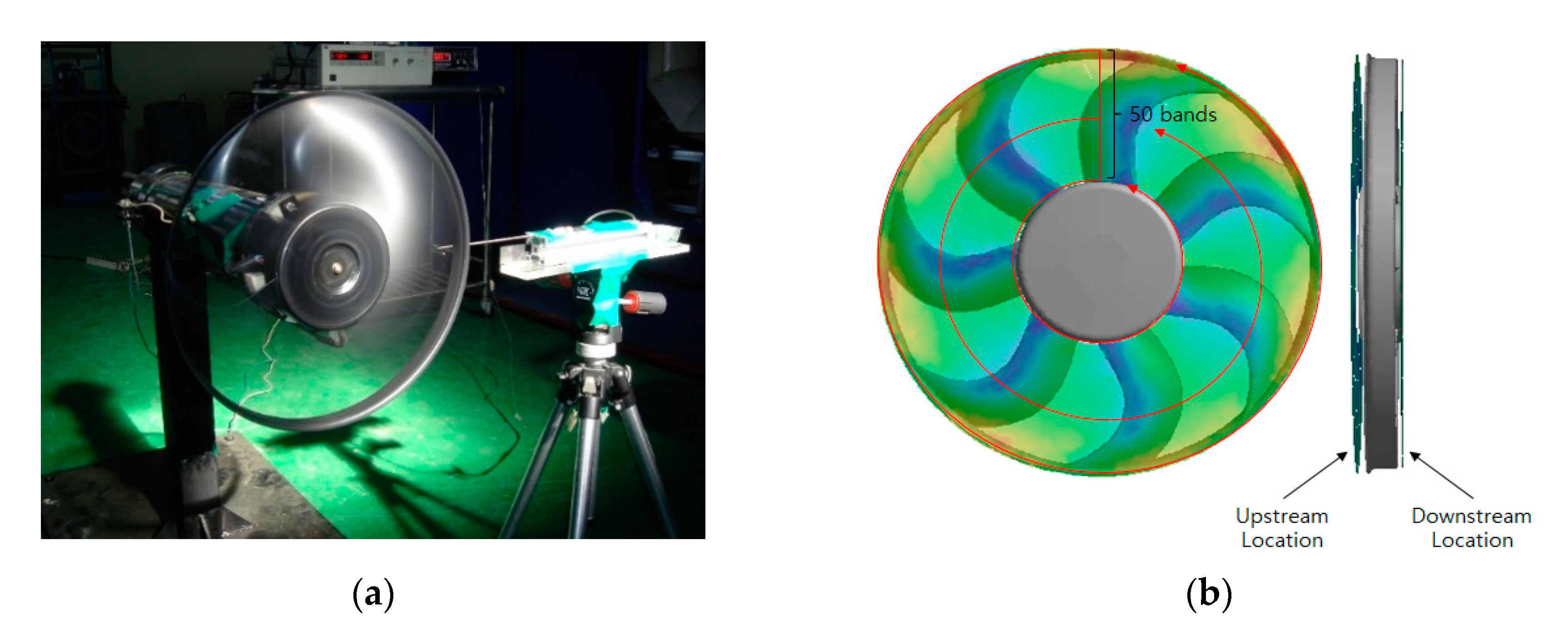
2.4. Experimental Methodologies for Velocity and Aerodynamic Noise Measurements

Figure 5a shows the experimental equipment for the velocity measurements using a single hot-wire probe of type I. The hot-wire anemometry is a technique used for measuring the fluid velocity. The hot-wire anemometer consists of two prongs with a wire stretched between them. For velocity measurements, the resistance measured with the singe hot-wire is converted into a voltage across an anemometer, and it is then saved in a computer as a digital file through a computer DAQ board. Single hot-wire calibration was performed, and its accuracy for several measurement values was within 5%. The hot-wire probe is located 5 mm away in the upstream at the front side of the hub and 3 mm away in the downstream at the back side. The data were measured at 1000 sampling rates per second for 5 s from the radius of r_h to r_t, and then averaged to obtain the velocity. Figure 5b illustrates that the velocity in the simulation was obtained by averaging all the data of a radial band in the circumferential direction, from the hub outside to the rig with radial bands of 50. The aerodynamic noise was measured at an anechoic room in Korea Advanced Institute of Science and Technology (KAIST). The FFT analysis of the measured data was performed on the temporal signals obtained with 5000 samples during approximately 174 revolutions, which induced spectral resolutions of 1 Hz [28].

3. Results and Discussion

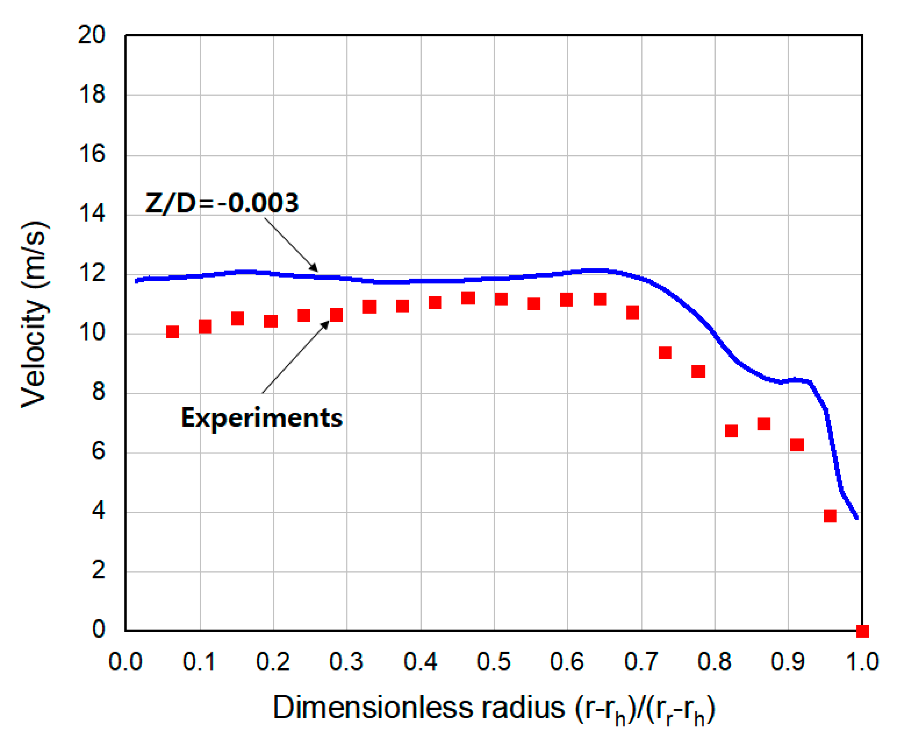
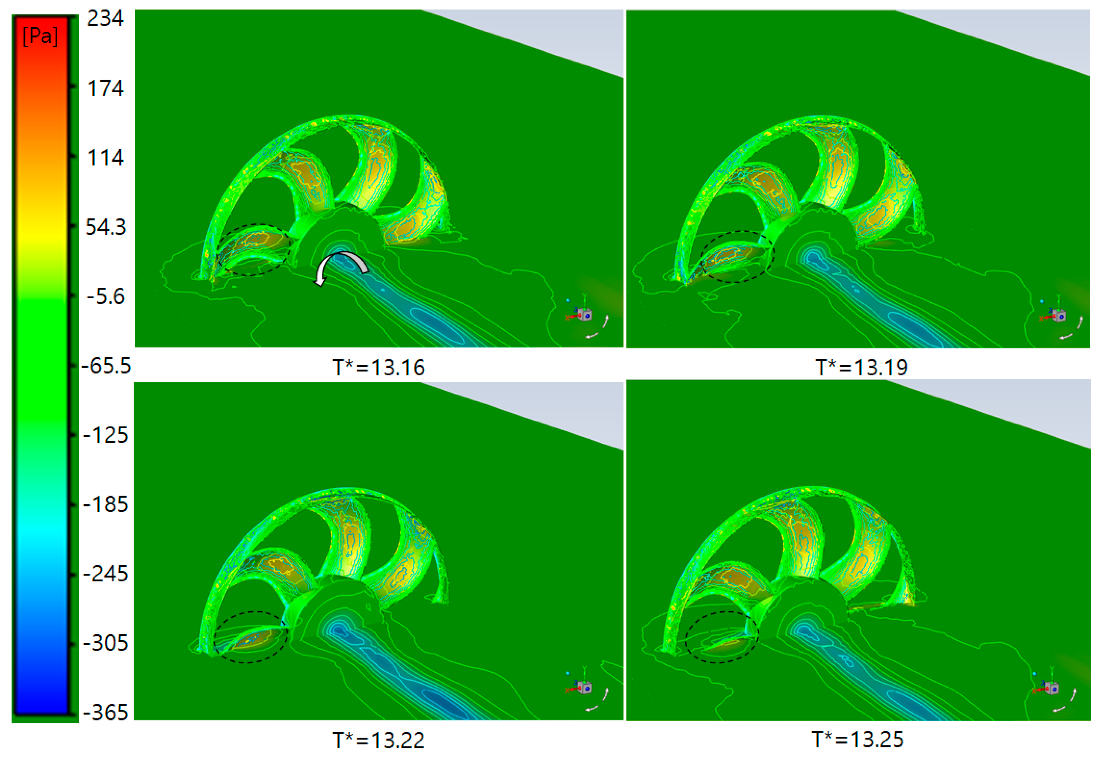
3.1. Flow Characteristics over an Axial Fan

The flow characteristics over the fan must be understood because the aerodynamic noise was generated by an unsteady flow. Figure 6 shows the iso-surface of the instantaneous vorticity magnitude of −2.81 × 10² at T* = 9.2. The fan blades generated a wide range of vorticities over the blades after a laminar separation of the bubbles on the surface of each blade consisting of slender airfoils from the root at tip. The presence of the vortices affected the resulting aerodynamic performance and noise. In general, the existence of the separation bubble on an airfoil is considered undesirable because it can have negative effects on the performance owing to the local alteration of the surface pressure distribution and lead to main flow unsteadiness if the bubble bursts [29,30].

Figure 7 shows the instantaneous pressure contours on the fan’s surface and the streamlines and velocity vectors in the X–Z plane at Z = 0 (T* = 9.2). Here, X, Y, Z, and D represent each direction of the X, Y, Z coordinates and the fan diameter, respectively, as indicated in the right lower end of Figure 7. The axial flow was more dominant at some locations of Z/D = 0.638 and 0.368 far away from the hub’s front side when the fan was rotating. However, at Z/D = 0.114 in the upstream, the radial flow near the ring rapidly flowed into the passages between the blades due to the low pressure of strongly pushing air into the downstream and allowed some dead zones around the ring to be formed, including the wake just after the hub. A comparatively higher pressure on the pressure side of the blade was generated, and the pressure difference caused a flow through the fan.

The simulation results for the velocities in the upstream and downstream were validated with experiments (Figure 8 and Figure 9). The flow increased more from Z/D = 0.638 to Z/D = 0.114 due to the increased pressure difference with the ambient pressure. The velocity at Z/D = 0.638 was approximately 1.2 m/s and increased to approximately 7.5 m/s at Z/D = 0.114. The velocity distribution at Z/D = 0.114 calculated from the LES in the upstream showed a comparatively good agreement with the experiments, except 0.75 and 0.92 of dimensionless radius, where the simulation results were slightly overpredicted due to the misalignment of measurement locations between the simulation and the experiment. As previously stated, the high velocities between 0.75 and 0.92 of dimensionless radius were confirmed due to the increase in the radial velocity (Figure 7). Similarly, the velocity distribution in the simulation in the downstream was overall overpredicted; however, it maintained a similar shape with the experiments. Compared to the upstream, the velocities at the same location between 0.75 and 0.92 of dimensionless radius were decreased due to the influence of the dead zone.

The pressure contours at the y = 0 section at different dimensionless times of T* = 13.16, 13.19, 13.22, and 13.25 based on one cycle of T* = 1 were illustrated by the pressure side of the fan’s blades and the wake region (Figure 10). Here, dimensionless time is defined as the ratio of the simulation time to the period corresponding to rotational speed of 2100 rpm. The pressure variations occurred between −365 Pa and 234 Pa, with a period of approximately 0.004082 s at the first BPF of 245 Hz. The instantaneous pressure contours indicated that a very small pressure pulsation caused by the vortices over the blades was present near the blades when the fan was rotating. A similar phenomenon was observed by Hu et al. [31] in the low-speed region of a rearview, where two rotating vortices were present, and the motion directions of both vortices opposed each other. Therefore, each blade caused the airfoil accelerated airflow and intensified the pressure fluctuation, thereby producing the aerodynamic noise.

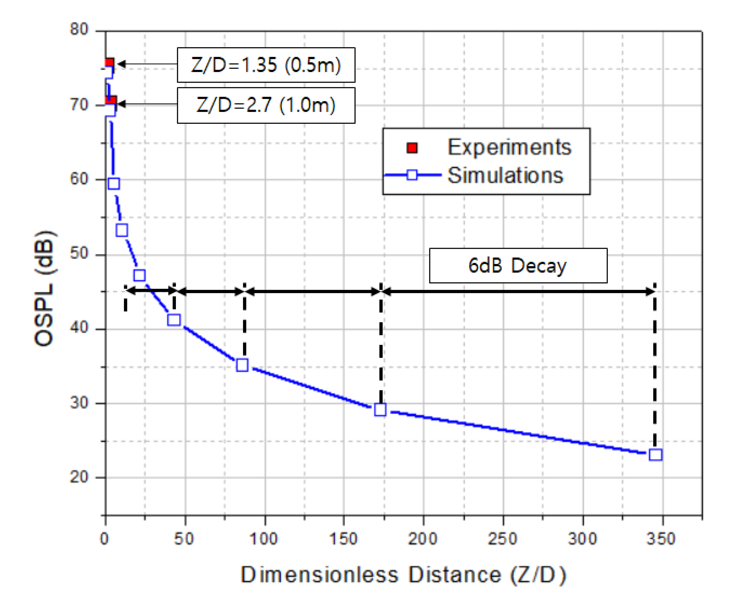
3.2. Aerodynamic Noise Characteristics

The fast Fourier transform (FFT) data were compared between the experiments and the simulations at the locations of 0.5 m and 1.0 m and θ = 90° in the downstream direction from the fan (Figure 11). The expression of 2$\times {\log }_{10}\left(\frac{P_{rms}}{P_{ref}}\right)$ was used to compute the SPL, where $P_{rms}$ and $P_{ref}$ denote the root mean square of the sound pressure and the reference of the sound pressure (20 $\times {10}^5 \mathrm{Pa})$, respectively. The FFT analysis was performed on the temporal signals obtained with 2004 samples during 8.87 revolutions in the simulations, which induced spectral resolutions of 4 Hz, compared with 1 Hz in the experiments. To obtain a frequency resolution in the simulations that is equivalent to that in the experiments requires four times more computational time than the approximately 168 h required for 13 revolutions. Thus, the difference in the resolution can affect the determination of the absolute noise level in each BPF. The experimental result at the location of 0.5 m showed that the highest SPL of 57.8 dB was observed at a 245 Hz frequency corresponding to the first BPF and its first and second harmonics of 53.8 dB and 47.9 dB at doubled and tripled frequencies of 490 Hz and 735 Hz, which corresponded to the 2nd and 3rd BPFs, respectively. Similarly, the location of 1.0 m also showed the highest SPL of 51.1 dB at the same frequency corresponding to the first BPF and its first and second harmonics of 46.9 dB and 40.4 dB at the doubled and tripled frequencies of 490 Hz and 735 Hz corresponding to the 2nd and 3rd BPFs, respectively. The experimental results illustrate that the dipole sources at each BPF had a major contribution to the generation of the fan’s aerodynamic noise. Furthermore, at the location of 1.0 m, SPL decreases of 6.7 dB, 6.9 dB, and 7.5 dB at each BPF were observed per distance doubling. The BPF noise level of the fan can be very intense and can vary with the number of blades (N) and the rotation speed of the fan (RPM):

BPF = N × RPM/60

(14)

The frequency histories of the SPL using the FW-H method based on the LES results were compared with the experimentally measured values and showed an acceptable agreement to 800 Hz. For the location of 0.5 m, the highest SPL of 66.6 dB at the first BPF was overpredicted compared to the experimental value of 57.8 dB. However, the peaks at the 2nd and 3rd BPFs were lower than those in the experiments. Similarly, for the location of 1.0 m, the highest SPL was 60 dB at the first BPF and became lower than that in the experiments at the 2nd and 3rd BPFs. These discrepancies might be due to the shorter data acquisition duration, particularly at high frequencies, and the insufficient mesh resolution close to the fan blades. Therefore, a longer data acquisition duration and sufficient mesh resolution may improve these discrepancies.

During the transient flow simulation, the time histories of the instant surface pressure values were written into the acoustic data files with which an operation was performed for the surface zones of the fan that were selected as acoustic sources. Figure 12 shows the SPL visualization of the fan noise source on the suction and pressure sides for the first BPF dipole sources that were between the 242.7 Hz and 246.6 Hz band range. A strong tonal noise existed near the leading edge of the blades under approximately Re = 9.75 × 10⁵ at the blade tip, which amounted to 111 dB SPL and a pressure side higher than the suction side in the SPL. This is expected to be caused by the separation in the leading edge of the airfoil consisting of the fan with the increasing radial velocity that resulted in the increasing angles of attack. According to Brooks et al. [32], at moderate angles of attack of the low Reynolds numbers, the flow separates from the trailing edge of the airfoil, thereby producing a trailing edge noise owing to shed turbulent vorticity. However, at very high angles of attack of the low Reynolds numbers, the separated flow near the trailing edge of the airfoil, generates a large-scale separation, thereby causing the entire airfoil to emit a low-frequency noise [33]. Therefore, the blade component is more dominant compared to the ring and the hub as dipole sources causing the tonal noise. The separation noise is considered to be of more major importance for the automotive axial fan when an improper fan design is present.

Figure 13 shows the predicted overall sound pressure level (OSPL) history of the dimensionless distance plotted in the blue line according to distance doubling downstream from the fan and the experimental OSPL values plotted in red dots. The OSPL is the equivalent SPL taken by integrating the SPLs across all frequencies. In the present study, frequencies up to 4000 Hz were considered. The results of the FW-H model showed good tendency with those of the wave theory equation in the far-field region after Z/D = 5.4, where the sound pressure produced by a point source decreased to 6 dB each time the distance from the point was doubled. The simulation results confirmed the 6 dB decay characteristic from Z/D = 5.4 to Z/D = 350 with distance doubling. The OSPL values at Z/D = 1.35 and 2.7 were 74.4 dB and 69.3 dB, respectively, and were a little underpredicted compared to the experimental data (i.e., 75.2 dB and 70.2 dB, respectively). The discrepancy came from the low resolution in high frequencies up to 4000 Hz. Unlike the far-field region, the near-field regions around the fan decreased approximately 5 dB to Z/D = 5.4 because the sound fields were complex, and the noise propagation did not develop well due to the reflecting wave by objects, such as equipment installation and walls [34]. Therefore, the sound pressure did not decrease as rapidly as it did in the free field. In other words, it decreased by less than 6 dB in the near-field region each time the distance from the sound source doubled.

Table 2. Predicted OSPL ratio of each component to the total dipole source of the fan at Z/D = 1.35 and 2.7.

Z/D	Fan (Blades + Rig + Hub)	Blades	Rig	Hub
1.35	74.39 (100%)	71.21 (69.3%)	55.92 (10.6%)	60.44 (20.1%)
2.70	69.25 (100%)	66.39 (71.6%)	51.25 (12.5%)	53.28 (15.8%)

shows the predicted OSPL ratio of each component (blades, rig, and hub) to the total dipole source of the fan at Z/D = 1.35 and 2.7 to analyze the contribution of each component. Each OSPL ratio was calculated using the SPL formula. The contribution of the dipole source to the tonal noise in the blades, rig, and hub was 69.3%, 10.6%, and 20.1%, respectively, at Z/D = 1.35. Furthermore, the blade’s contribution to the noise increased to 71.6% at Z/D = 2.7 when the distance doubled. In the present study, the quadruple source due to the unsteady momentum transport in turbulent flow was disregarded because of the subsonic flow caused by the fan blades. According to Mo and Lee [35], the dipole source in the rotating wind turbine blades was more dominant when the incoming velocity was low, but became less predominant for a higher wind speed. In conclusion, the dipole source caused by the fan blades in normal conditions plays an important role in tonal noise and is the main sound source at a low frequency.

4. Conclusions

LES of an automotive axial cooling fan with seven blades in the near-field and noise prediction to the far-field using FW-H method were carried out to provide a better understanding of unsteady flow and aerodynamic noise characteristics. The computational domain had a cylinder type consisting of rotating and stationary parts with a pressure condition with 0.2% turbulence intensity and the analysis was performed under a constant rotational speed of 2100 rpm. The reliability and validity of the simulations were verified with experimentally measured data. Comparatively good agreements were achieved for the velocity distributions in the upstream and downstream and the aerodynamic noise of SPLs at two different receivers. However, for the further reduction of these discrepancies in the unsteady flow and aerodynamic noise, a longer data acquisition duration and sufficient mesh resolution may be required. The quadruple source due to the unsteady momentum transport in turbulent flow was disregarded owing to the subsonic flow caused by the fan blades, and only the dipole source due to the fan surface was considered for efficient and less expensive computation. Important findings arising from this research are as follows:

(1) The radial flow near the fan’s ring was accelerated into the passages between the blades owing to the low pressure of the strongly pushing air from Z/D = 0.638 in the downstream to Z/D = 0.114 in the upstream; this caused an uneven velocity distribution in the upstream and downstream, and enabled the formation of a few dead zones around the ring, including the wake immediately after the hub. The simulation results for the velocity distributions were slightly overpredicted due to the misalignments of the measurement locations. Additionally, the instantaneous pressure pulsation was limited to a significantly small range of −365 Pa and 234 Pa owing to the vortices over the blades.

(2) This study experimentally confirmed that the highest SPL was 57.8 dB at 245 Hz of the first BPF, and its first and second harmonics were 53.8 dB and 47.9 dB at the 2nd and 3rd of 409 Hz and 735 Hz, respectively. At the location of 1.0 m, the SPL decreased by 6.7 dB, 6.9 dB, and 7.5 dB at each BPF per distance doubling. Therefore, the dipole sources emitted from the fan made a major contribution to the aerodynamic noise generation. In contrast, the simulation results demonstrated that the highest SPL was overpredicted by 8.6 dB and the peaks at the 2nd and 3rd BPFs were underpredicted in comparison with the experimental results at the location of 0.5 m due to the shorter data acquisition duration, particularly at high frequencies, and the insufficient mesh resolution close to the fan blades.

(3) A strong tonal noise numerically existed near the leading edge of the blades at the tip and amounted to 111 dB SPL. Furthermore, the pressure side of the blades was higher than the suction side in the SPL. This was a result of the large-scale separation near the leading edge of the airfoils caused by the increasing angles of attack with the increasing radial velocity near the ring, which caused the entire airfoil to emit a low-frequency noise. Therefore, the blade component was more dominant than the ring and the hub as a dipole source causing the tonal noise. The separation noise is considered to be of greater importance for the automotive axial fan when an improper fan design is present.

(4) The numerical observation revealed that a 6 dB decay in the far-field region existed from Z/D = 5.4 to Z/D = 350 with distance doubling, whereas approximately 5 dB in the near-field region decreased less. The sound fields near the fan were complex, and the noise propagation did not develop well owing to the reflecting wave. Therefore, the sound pressure decreased by less than 6 dB in the near-field region compared to that in the far-region each time the distance from the sound source doubled. Additionally, the contribution of the dipole source to the tonal noise in the blades was the most predominant, reaching 69.3% at Z/D = 1.35 and 71.6% at Z/D = 2.7, in comparison with the ring and hub components.

Thus, the results of this study can help designers in designing axial fans and optimizing the blade shape of the fan to achieve low noise and high performance. In the future, further investigations into the effects of the blade and ring shapes will be conducted to improve the aerodynamic noise.

References

1. Available online: https://repairpal.com/radiator-fan-assembly (accessed on 6 June 2020).
2. Allam, S.; Abom, M. Noise reduction for automotive radiator cooling fans. In Proceedings of the FAN 2015—International Conference on Fan Noise, Technology and Numerical Methods, Institution of Mechanical Engineers, Lyon, France, 17 April 2015. [Google Scholar]
3. Abbas, A.; Elwali, W.; Haider, S.; Dsouza, S.; Sanderson, M.; Segan, Y. CAE Cooling Module Noise and vibration Prediction Methodology and Challenges. SAE Tech. Pap. 2020. [Google Scholar] [CrossRef]
4. Chanaud, R.C.; Muster, D. Aerodynamic noise from motor vehicles. J. Acoust. Soc. Am. 1975, 58, 31–38. [Google Scholar] [CrossRef]
5. Neise, W. Review of Fan Noise Generation Mechanisms and Control Methods, Fan Noise Symposium; CETIM: Seulis, France, 1992. [Google Scholar]
6. Blake, W.K. Mechanics of Flow-induced Sound and Vibration. Vol. 2: Complex Flow Structure Interaction; Academic Press Inc.: London, UK, 1986. [Google Scholar]
7. Goldstein, M.E. Aeroacoustics; McGraw-Hill International: New York, NY, USA, 1976. [Google Scholar]
8. Ffowcs-Williams, J.E. Aeroacoustics. Ann. Rev. Fluid Mech. 1977, 9, 447–468. [Google Scholar] [CrossRef]
9. Sharland, I.J. Sources of noise in axial flow fans. J. Sound Vib. 1964, 1, 302–322. [Google Scholar] [CrossRef]
10. Lighthill, M.J. On sound generated aerodynamically: I. general theory. Proc. Roy. Soc. Lond. A 1952, 211, 564–587. [Google Scholar]
11. Lighthill, M.J. On sound generated aerodynamically: II. Turbulence as a source of sound. Proc. R. Soc. Lond. A 1954, 222, 1–32. [Google Scholar]
12. Lighthill, M.J. Jet noise. The Wright Brothers Lecture of 1963. AIAA J. 1963, 1, 1507–1517. [Google Scholar]
13. Lilley, G.M. On the noise from jets, Noise Mechanism, AGARD-CP-131. AGARD Conf. Proc. 1974, 13, 1–12. [Google Scholar]
14. Curle, N. The influence of solid boundaries upon aerodynamical sound. Proc. Roy. Soc. Lond. A 1955, 231, 505–514. [Google Scholar]
15. Brentner, K.S.; Farassat, F. An analytical comparison of the acoustic analogy and kirchhoff formulations for moving surfaces. Aiaa J. 1988, 36, 1379–1386. [Google Scholar] [CrossRef] [Green Version]
16. Ffowcs-Williams, J.E.; Hawkings, D.L. Theory relating to the noise of rotating machinery. J. Sound Vib. 1968, 10, 10–21. [Google Scholar] [CrossRef]
17. Ffowcs-Williams, J.E.; Hawkings, D.L. Sound generation by turbulence and surfaces in arbitrary motion. Proc. Roy. Soc. Lond. 1969, 264, 321–342. [Google Scholar]
18. Fukano, T.; Kodama, Y.; Senoo, Y. Noise generated by low pressure axial flow fan. I.: Modeling of the turbulent noise. J. Sound Vib. 1977, 50, 63–74. [Google Scholar] [CrossRef]
19. Fukano, T.; Kodama, Y.; Takamatsu, Y. Noise generated by low pressure axial flow fan. II.: Effects of number of blades, chord length and camber of blade. J. Sound Vib. 1977, 50, 75–88. [Google Scholar] [CrossRef]
20. Argüelles, D.K.M.; Fernández, O.J.M.; Blanco, M.E.; Santolaria, M.C. Numerical prediction of tonal noise generation in an inlet vaned low-speed axial fan using a hybrid aeroacoustic approach. J. Mech. Eng. Sci. 2009, 223, 203–210. [Google Scholar] [CrossRef]
21. Vondervoort, R.V.D. Prediction of Aerodynamic Performance and Noise Production of Axial Fans. Master’s Thesis, University of Twente, Enschede, The Netherlands, 2015. [Google Scholar]
22. Park, S.M.; Ryu, S.Y.; Cheong, C.; Kim, J.W.; Park, B.I.; Ahn, Y.C.; Oh, S.K. Optimization of the orifice shape of cooling fan units for high flow rate and low-level noise in outdoor air conditioning units. Appl. Sci. 2019, 9, 5207. [Google Scholar] [CrossRef] [Green Version]
23. Moreau, S. Direct noise computation of low-speed ring fans. Acta Acust. United Acust. 2019, 105, 30–42. [Google Scholar] [CrossRef]
24. Franzke, R.; Sebben, S.; Bark, T.; Willeson, E.; Broniewicz, A. Evaluation of the multiple reference frame approach for the modelling of an axial cooling fan. Energies 2019, 12, 2934. [Google Scholar] [CrossRef] [Green Version]
25. Smagorinsky, J. General circulation experiments with the primitive equations 1. The basic experiment. Mon. Weather Rev. 1963, 91, 99–164. [Google Scholar] [CrossRef]
26. Hinze, J. Turbulence, 2nd ed.; McGraw-Hill: New York, NY, USA, 1975. [Google Scholar]
27. Lilly, D. A proposed modification of the Germano subgrid-scale closure method. Phys. Fluids A Fluid Dyn. 1992, 4, 633. [Google Scholar] [CrossRef]
28. Kim, K.Y. A Study on the Prediction Method of Shroud Fan Broadband Noise. Ph.D. Thesis, Korea Advanced Institute of Science and Technology, Daejeon, Korea, 2007. [Google Scholar]
29. Almutairi, J.H.; Jones, L.E.; Sandham, N.D. Intermittent bursting of a laminar separation bubble on an airfoil. Aiaa J. 2010, 48, 414–426. [Google Scholar] [CrossRef]
30. Lou, W.; Hourmouziadis, J. Separation bubbles under steady and periodic-unsteady main flow conditions. J. Turbomach. 2000, 122, 634–643. [Google Scholar] [CrossRef]
31. Hu, X.; Guo, P.; Wang, Z.; Wang, J.; Wang, M.; Zhu, J.; Wu, D. Calculation of external vehicle aerodynamic noise based on les subgrid model. Energies 2020, 13, 1822. [Google Scholar] [CrossRef]
32. Brooks, T.; Pope, D.; Marcolini, M. Airfoil Self-Noise and Prediction. Technical Report; NASA Reference Publication: Hampton, VA, USA, 1989; p. 1218. Available online: https://ntrs.nasa.gov/search.jsp?R=19890016302 (accessed on 6 June 2020).
33. Oerlemans, S. Wind Turbine Noise: Primary Noise Sources. Technical Report; National Aerospace Laboratory NLR(Royal Netherlands Aerospace Centre): Amsterdam, The Netherlands, 2011; Available online: https://reports.nlr.nl/xmlui/bitstream/handle/10921/117/TP-2011-066.pdf (accessed on 6 June 2020).
34. Ray, E.F. Industrial Noise Series Part IV: Modeling Sound Propagation; Stoughton Chamber of Commerce: Stoughton, WI, USA, 2010. [Google Scholar]
35. Mo, J.O.; Lee, Y.H. Numerical simulation for prediction of aerodynamic noise characteristics on a HAWT of NREL phase VI. J. Mech. Sci. Technol. 2011, 25, 1341–1349. [Google Scholar] [CrossRef]
Figure 1. Automotive cooling axial fans.
Applsci 10 05432 g001
Figure 2. The actual product of an axial fan (a) and corresponding geometric cad model (b).
Applsci 10 05432 g002
Figure 3. Simulation domains consisting of stationary and rotating regions and corresponding analysis model with hexahedral and tetrahedral elements.
Applsci 10 05432 g003
Figure 4. y+ value distribution on suction and pressure sides of the axial fan.
Applsci 10 05432 g004
Figure 5. Experimental equipment for velocity measurements (a) and numerical velocity-averaged method with radial bands of 50 (b).
Applsci 10 05432 g005
Figure 6. Iso-Surface of instantaneous vorticity magnitude at T* = 9.2.
Applsci 10 05432 g006
Figure 7. Instantaneous pressure contours on the fan’s surface, and streamlines and velocity vectors in X–Z plane at Z = 0 m (T* = 9.2).
Applsci 10 05432 g007
Figure 8. Velocity distributions at each section at y = 0 section in the upstream and comparison with experiments.
Applsci 10 05432 g008
Figure 9. Comparison of a velocity distribution with experiments at y = 0 section in the downstream.
Applsci 10 05432 g009
Figure 10. Pressure contours on the pressure side of the fan’s blades an in the wake region at y = 0 section at different dimensionless times of T* = 13.16, 13.19, 13.22, and 13.25.
Applsci 10 05432 g010
Figure 11. Frequency histories of SPL at 0.5 m (left) and 1m (right), θ = 90° in the downstream.
Applsci 10 05432 g011
Figure 12. SPL visualization of the fan noise source on the suction (left) and pressure (right) sides between 242.7 Hz and 246.6 Hz band range.
Applsci 10 05432 g012
Figure 13. Overall sound pressure level (OPSL) history of the dimensionless distance by the Ffowcs-Williams and Hawkinbygs (FW-H) model at the various receivers with doubling of distance in the downstream region and the comparison with experiments at Z/D = 1.35 and 2.7 corresponding to each location of 0.5 and 1.0 m, respectively.
Applsci 10 05432 g013