Thermometry in a Multipole Ion Trap

Featured Application

In this work, we present a versatile method to determine the translational temperature of ions trapped in a multipole ion trap. The temperature of the trapped ions is mapped onto their time of flight to the detector. Unlike other ion-thermometry techniques, e.g., Doppler spectroscopy, this method is time-efficient and can be applied to any ionic species, without relying on the availability of suitable optical transitions.

Abstract

We present a characterization of the ions’ translational energy distribution in a multipole ion trap. A linear mapping between the energy distribution of the trapped ions onto the ions’ time-of-flight (TOF) to a detector is demonstrated. For low ion temperatures, a deviation from linearity is observed and can be attributed to the emergence of multiple potential minima. The potential landscape of the trapped ions is modeled via the finite element method, also accounting for subtleties such as surface-charge accumulation. We demonstrate the validity of our thermometry method by simulating the energy distribution of the ion ensemble thermalized with buffer gas using a Molecular Dynamics (MD) simulation. A comparison between the energy distribution of trapped ions in different multipole trap configurations—i.e., with hyperbolic rods, cylindrical rods, and cylindrical wires—is provided. With these findings, one can map the temperature of the trapped ions down to the Kelvin regime using their TOF distributions. This enables future studies on sympathetic cooling and chemical reactions involving ions in multipole traps.

1. Introduction

Developments in the field of trapped particles have enabled the exploration of dynamical processes under the action of diverse short-range and long-range interactions. A detailed characterization of the spatial distribution and energy distribution of these trapped particles is imperative to investigate phenomena in ultracold chemistry [1,2,3,4,5,6,7,8], astrophysics [9], as well as astrochemistry [10], including the formation and evolution of the interstellar medium (ISM) [11,12,13,14,15]. For charged particles trapped in multipole ion traps, the measurement of temperature-dependent ion mobility and rate coefficients is one of the key methods to characterize the temperature of the ions [16]. With advances in the application of electrostatic lenses, another method called velocity map imaging became feasible such that ions with same initial velocity in the trap could be mapped onto the same point on the detector [17]. Similar to atoms, the phase space distribution of the trapped ions with closed optical transitions can also be characterized via Doppler-spectroscopy [18,19,20,21,22,23]. However, this is limited to only a number of atomic cations. In case of molecular anions, a detailed characterization for the internal thermometry via photodetachment techniques exists [24]. However, due to the rethermalization of the ions with the black-body radiation, the temperature of ions in the external and internal degrees of freedom are not necessarily the same. Recent work [25] measured the translational temperature of hydroxyl (OH${}^{-}$) anions via the Doppler width of an overtone transition, but this method is time-intensive and requires an exact knowledge of the overtone transition frequency.

In this work, we put forward a versatile tool to characterize the translational temperature of ions trapped in a multipole ion trap by mapping the ions’ time-of-flight (TOF) to the detector. Here, we describe an octupole radio frequency (rf) wire trap in a Hybrid Atom–Ion trap (HAI-trap) setup. We start by detailing the experimental setup and the ion trap assembly in Section 2 and Section 3, respectively. The current setup is an improved version of the earlier design described in [26]. Following the description of the trap, we investigate the potential landscape created by a multipole wire trap and traps with ideal cylindrical or hyperbolic rods in Section 4. We further compare the influence of different trap geometries on the final energy distribution of the trapped ions after interaction with a buffer gas. Then, in Section 5, we extend our investigations to the HAI-trap setup, where the 3-dimensional (3D) model of the system is used to simulate potential landscape in the trap, including surface charges that accumulate on the plastic components of the trap. The ion distributions obtained via the simulated potentials are compared with the measured ion distributions obtained via photodetachment tomography [27,28]. It is shown that the spatial energy distribution of ions in the trap can be mapped onto the ions’ time-of-flight to the detector, including the effect of multiple regions of potential minima that arise in multipole ion traps (with the pole order $>2$). Independent of the trapped ionic species, this technique is time-efficient and can be applied to any system without relying on the existence of suitable transitions for determining the ions’ motional temperature.

2. Overview of the Experimental Setting

A schematic representation of our experimental setup is shown in Figure 1. The ion source consists of a pulsed piezo valve, which injects a gas pulse into the vacuum system. In the current setup, a modified version of the design introduced by [29] is used. By actively controlling the discharge voltage and the gas flow into the vacuum chamber, a variety of ionic species can be created depending on the gas mixture used. Our benchmark system is the hydroxyl anion, which serves as our system of interest for the rest of this work. For the creation of hydroxyl anions, argon gas mixed with water vapor is used in the reservoir before the nozzle of the gas inlet. As the ions exit the source, they are guided via ion optics towards a Wiley–McLaren-based time-of-flight mass spectrometer, which is operated in a pulsed mode. Here, the ions are accelerated orthogonally with respect to their initial trajectory and are then separated in the time domain based on their mass-to-charge ratio. The ions are then focused through a pinhole into the next chamber where they are loaded into an octupole wire trap.

The trap assembly is explained in detail in Section 3. A 3-dimensional (3D) model of the wire trap is illustrated in Figure 2a, and a qualitative representation of the potential during loading, trapping, and extraction of the ions is shown in Figure 2b. The mass selection of the ions is done by switching the entrance endcap of the trap between a high and low potential in order to load the desired species. As the ions approach the trap, the entrance endcap electrode is set to a lower potential. Once the ions enter the trap, the entrance endcap electrode is switched to a higher potential, thus confining the ions in the trap axially.

In order to increase the trapping efficiency of the ions, a pulse of helium buffer gas is injected into the trap. This not only greatly enhances the number of ions trapped, but also ensures that the hot ions produced from the plasma discharge source are properly thermalized and lie in their vibrational ground state. This serves as the starting condition for the ion ensemble which can then be overlapped with a cloud of laser-cooled rubidium atoms. The implementation and characterization of the atom trapping setup is detailed in [30]. Additionally, a far-threshold laser beam can be shone onto the ions in order to characterize their spatial density distribution via photodetachment tomography [27].

Depending on the nature of the experiment, the ions can be confined in the trap for varying amounts of time. The interaction with laser-cooled atoms and/or a laser beam results in the change of the ions’ energy distribution which is recorded by extracting the ions from the trap and measuring the spread in the TOF distribution. The ions are extracted by lowering the potential on the exit endcap electrode and exit shielding plate close to the detector. Furthermore, the entrance shielding plate is switched to a higher potential to facilitate an additional acceleration of the ions towards the ion detector. In our case, a microchannel plate (MCP) is used to detect the arrival time of the individual ions. It is imperative to note that the ion detector counts single ion events, and does not integrate the signal. This is critical for comparing the measured ion distributions to those obtained from the simulations. (An integrator would introduce an additional broadening of the detected distribution). The width of this TOF distribution recorded on the detector can provide a direct mapping to characterize and quantify ions’ energy distributions.

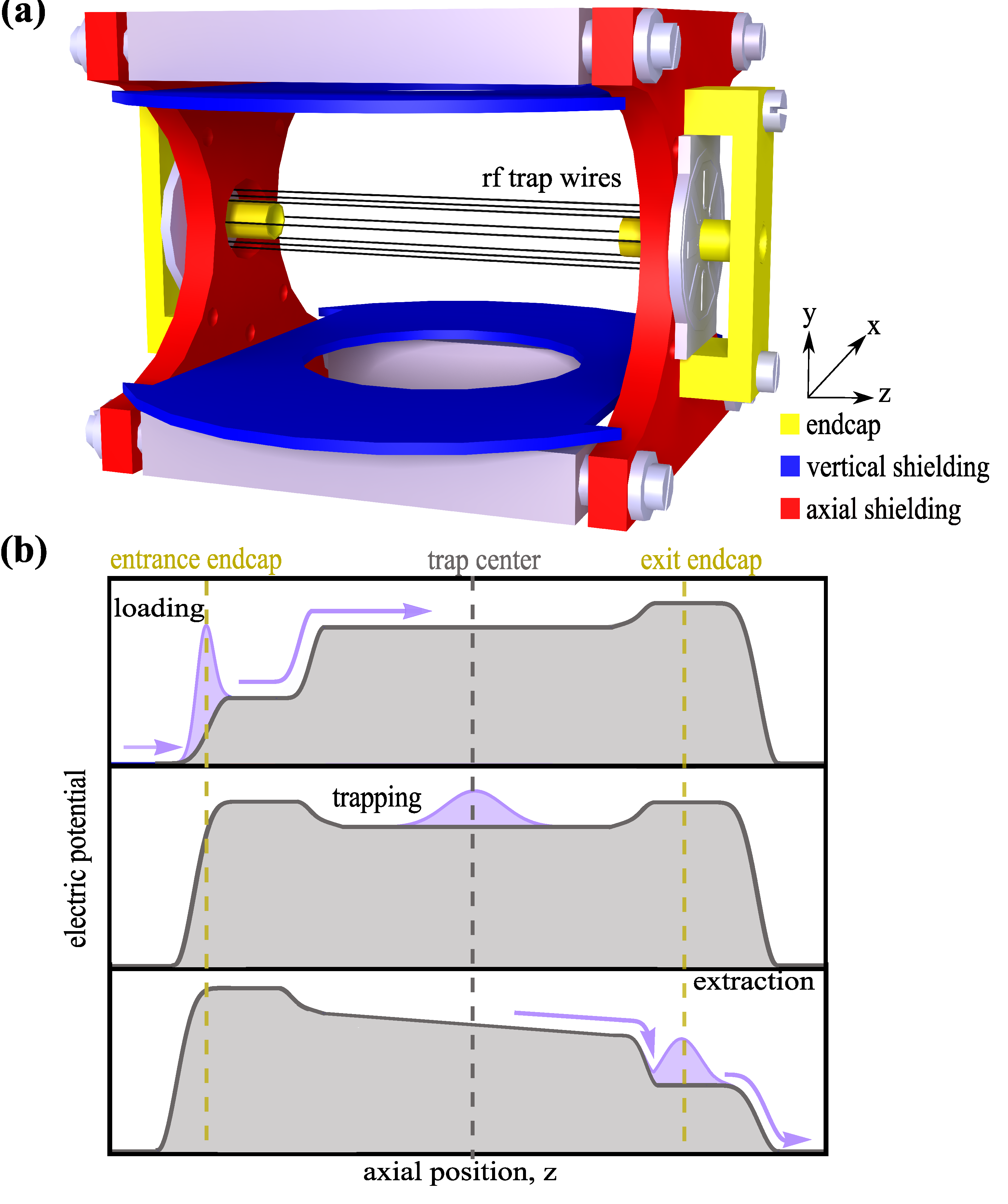
3. Description of the Ion Trap

The 3D model of the trap assembly is shown in Figure 2a. The octupole trap consists of eight gold-coated molybdenum wires with a diameter of 100 $\mathsf{\mu }\mathrm{m}$. They are symmetrically placed around the trap axis on a circle with radius of 3 $\mathrm{m}\mathrm{m}$. The wires are soldered onto a printed circuit board (PCB). A radio-frequency field is applied to the trap wires, along with an additional static voltage as an offset. The offset chosen corresponds to the voltages used in the Wiley–McLaren acceleration stage, which lowers the kinetic energy of the incoming ions such that the trapping potential can confine them. While the static voltage applied to the endcap electrodes provides axial confinement to the ions, the radio-frequency field applied to the wires confines the ions radially, such that the ions experience a position-dependent field proportional to $r^{2n-2}$, where n is the pole order of the ion trap, with $n=4$ for an octupole trap. The potential that the ions experience governs their spatial density distribution. Thus, while they are Gaussian-distributed in the axial direction due to the harmonic potential in this direction, they are described by a super-Gaussian distribution of order six in the radial direction [31].

The total potential exhibits a local maximum at the center of the trap along with off-center minima [32]. While the endcaps create a necessary confining potential in the axial direction, they also create a deconfining potential in the radial direction, which exhibits $r^2$ dependency close to the center [33]. This is a feature common to all multipole traps with $n>2$, and not only to octupole wire traps, thus creating multiple regions of local minima called “pockets”.

In addition to the rf wires and endcap electrodes, the trap consists of a set of vertical and axial shielding plates. The vertical shielding plates prevent the grounded MOT coils (not shown) from pulling down the potential in the trap center. The hole in the plates provide optical access for laser beams to create an MOT. The axial shielding plates provide the flexibility to shift the ion cloud during trapping or giving them additional acceleration during extraction, thus increasing the detection efficiency. The axial shieldings are important for controlling the slope of the potential during extraction, as seen in Figure 2b. The voltages applied to the endcap electrodes and shielding plates are optimized such that the trapped ion cloud is initially exposed to a linear acceleration region during extraction. This is necessary for obtaining a symmetric TOF spread. Additionally, the axial shieldings can also be used to modify the potential topology for the extraction process to enhance the mass resolution of the system. This is particularly useful for exploring systems with higher masses, where multiple ionic species are simultaneously trapped.

A wire trap offers the advantage of providing optical access for laser beams for hybrid atom–ion experiments, and an octupole trap provides a large central field-free region where the influence of radio-frequency heating is reduced. However, one feature of wire traps that needs to be noted while designing a trap assembly is that all nearby electrodes and grounded plates will influence the potential, in the region enclosed by the wires, drastically. This effect is diminished for a trap using thicker rods, as the penetration of outer electrodes is greatly reduced.

As opposed to the traps with wires, the ones using ideal cylindrical rods and hyperbolic rods are mechanically more robust. The large size difference between wire and rod traps raises the question of how the potential landscape deviates in these different types of trap. To understand the differences in the potential between a wire trap and the more commonly used multipole trap consisting of thicker cylindrical rods, a detailed comparison between traps with wires and cylindrical or hyperbolic rods is subsequently described in Section 4.

4. Comparison between Wire and Rod Traps

In order to describe the confining potential created by an rf field and the physics governing the dynamics in an ion trap, the adiabatic approximation is used. Here, the ion motion is split into a fast oscillatory motion, also called micromotion; and a slow drift motion in the confining ponderomotive potential, called macromotion. Henceforth, the potential created by rf traps can be expressed as an effective conservative potential (averaged over one oscillation period), given by [34]

$$V_{\mathrm{eff}}(\overrightarrow{R}\left(t\right))=\frac{e^2}{2m{\omega }^2}\langle \overrightarrow{E}{(\overrightarrow{R}\left(t\right),t)}^2\rangle .$$

(1)

Here, $\overrightarrow{R}\left(t\right)$ describes the trajectory of the macromotion, $\overrightarrow{E}$ is the time-dependent electric field, e is the electronic charge, and m is the mass of the ion. This results in a pseudo-static effective potential, which can approximately describe the ion trajectories in different multipole traps. This approximation allows the comparison between different trap types via a static potential. The three trap types under consideration are the ideal hyperbolic trap, a trap consisting of cylindrical rods, and a trap using wires. A geometric comparison between the trap types is given in Figure 3a.

In order to replicate the curvature of the ideal multipole potential to first and second order, the radius of the cylindrical rods used must fulfill the following relation [34,35]:

$$\rho =\frac{r_0}{n-1}.$$

(2)

For our wire trap with 100 $\mathsf{\mu }\mathrm{m}$ diameter wires and a distance from the trap center of 3 mm, the ideal rod diameter is 1.5 mm, which is more than an order of magnitude larger than the wire size, and thus, Equation (2) is far from being fulfilled.

Due to the vast geometric differences between the three mentioned rod shapes, it is not trivial to predict if and how the potential landscape differs in the different trap types. In an attempt to investigate these differences, we used COMSOL Multiphysics to simulate infinitely long traps without endcaps. For details on the COMSOL simulations, see Appendix A. The geometries are chosen as seen in Figure 3a, with the hyperbolic and cylindrical rod trap having the same inscribed radius of 2.25 mm, and the wire trap lying concentrically inside the rod. The simulated electric fields are used to calculate an effective potential via Equation (1) assuming OH${}^{-}$ ions and a trap frequency f of 5 MHz. The resultant potential was then averaged over the azimuthal angle and the voltage was varied until the difference in the average effective potential between the hyperbolic trap and the rod/wire trap was minimized.

As a result, it was observed that in order to match the potential created by hyperbolic rods, the ideal rod trap needs a factor of 1.01, or about a 1% increase in the voltage; while the wire trap needs a voltage 5.4 times higher for the same. Thus, with a suitably higher voltage, it is possible to match the averaged potential. However, the ideal rod trap and wire traps exhibit maxima and minima over the azimuthal angle corresponding to the position of the rods/wires and the space in between them. These results are depicted in Figure 3b. The effective potential for the different trap configurations as a function of the azimuthal angle at three different radii (from the center of the trap) is shown. These radii are also marked in Figure 3a. At each of these radii, it can be seen that the amplitude of modulations in the wire trap exceeds those in the rod traps. Furthermore, these distortions become more prominent as one goes radially outwards in the case of a cylindrical rod/wire trap. As a consequence of these deviations, the minimum voltage for stable trapping of ions increases for a cylindrical rod trap, and is even further increased for a wire trap.

In order to estimate the influence of the deviations from the ideal hyperbolic potential on the temperature of ions in the trap when they encounter a neutral collision partner, a Monte-Carlo buffer gas simulation for all three trap configurations was performed. The voltages used are the same as the ones previously used to match the potential landscape of a hyperbolic trap with 50 $\mathrm{V}$ rf amplitude. These simulated, matched voltages are used to calculate the electric field vectors, which are then loaded into a home-built script. Subsequently, the ion trajectories are calculated, and a classical, hard-sphere-based collision model is used to simulate the collisions with a buffer gas. For details on the Molecular Dynamics simulations, see Appendix B. In our case, we investigate the thermalization of OH${}^{-}$ ions with a room-temperature helium buffer gas. The mean speed of the ions is obtained via the Molecular Dynamics (MD) simulations. The resultant energy distribution is demonstrated in Figure 4. The temperature of the ion ensemble T is calculated from the ions’ mean speed ($\overline{v}$) as

$$T=\frac{\pi m{\overline{v}}^2}{8k_{\mathrm{B}}},$$

(3)

where $k_{\mathrm{B}}$ is the Boltzmann constant (We hereby use Equation (3) to define the notion of temperature, as well as in case of the emerging nonthermal distributions.). In all three cases, a temperature of 366 $\mathrm{K}$ was obtained, with the deviations between the traps being $<1$$\mathrm{K}$. The insignificant deviation in the temperature between the different types of traps can be explained via the mean radial extension of ions in the trap which, in the simulations, is 0.24$·r_0$ (also depicted in Figure 3a). This means that the ions primarily explore the innermost region of the trap, and spend only a little time in the outer region of the trap, where the modulations in the effective potential are relatively higher. In Figure 4, the dashed black line represents an analytical Maxwell–Boltzmann distribution at 366 $\mathrm{K}$ [36]. Furthermore, it can be inferred that the ions energy distribution is not perfectly described by a Maxwell–Boltzmann distribution and exhibits a nonthermal behavior. The simulated temperature is significantly higher than the temperature of the buffer gas at 293 $\mathrm{K}$. This effect is dependent on the multipole order and is well-investigated in previous works [37], amounting it to the collision of ions in the micromotion-dominated region of the rf trap.

In view of the above results, it can be assumed that the main heating mechanism is the micromotion-dominated rf heating which causes the ions to gain additional energy when colliding in the rf field. In the case of thermalization of ions with a neutral buffer gas at room temperature, the deviations prevalent in the rod or wire trap from the ideal hyperbolic potential can be neglected.

5. Translational Temperature Determination in HAI-Trap

The mapping of the ion ensemble’s energy distribution in the trap onto the TOF spread of the extracted ions demands a more sophisticated model of the setup. Thus, the 3D trap assembly of the HAI-trap experiment with all the electrodes including the endcaps and shieldings, as described in Section 3, are accounted for in the COMSOL simulation. In this section, firstly, the translational temperature of the ions is simulated via an MD simulation. The energy distribution thus obtained is then characterized via a photodetachment tomography of the ions’ spatial distribution. The energy and spatial distribution is then used to determine the influence of surface charges that can accumulate on the printed circuit boards (PCBs) in the trap assembly. Subsequently, the mapping of the ions’ TOF distribution onto the detector and the obtained correlation between the spread of TOF distribution and the ions’ translational temperature is discussed. For details on the COMSOL simulations, see Appendix A; and for details on the Molecular Dynamics simulations, see Appendix B.

5.1. Energy Distribution of Trapped Ions

A 3D model of the trap is imported into the COMSOL environment to obtain the potential landscape created by the static voltages of the various electrodes. Subsequently, in the Monte-Carlo simulation, this static potential is then combined with the potential created by the rf field to simulate the energy distribution, as shown in Figure 5. In case of OH${}^{-}$ thermalizing with helium buffer gas, the temperature obtained from the distribution is 373 $\mathrm{K}$, and is a few Kelvin higher than that of the infinitely long wires (no endcaps). This stems from the fact that the static voltages push the ions into the rf field near the endcaps. While this relative effect is minimal at room temperatures, it is shown to become more pronounced and critical for cryogenic traps, where collisions occur in Kelvin regime [37]. While the dynamics of the ions in the low-to-mid energy range are well-represented by a Maxwell distribution, the high-energy tail of the distribution can be described with a Tsallis distribution [38].

5.2. Spatial Distribution from Photodetachment Tomography

The difference between the two distributions, shown in Section 5.1, can be further characterized by mapping out the spatial ion distribution along the cylindrical axis of the ion trap via a far-threshold photodetachment tomography. This technique determines the density distribution without relying on a closed cycling transition and precise imaging systems. If the photon energy of the laser is above the electron affinity of the anion, then the process of laser-induced photodetachment, OH${}^{-}$ + h$\nu \to$ OH + e${}^{-}$, causes neutralization of the anion—as a result, it is lost from the trap.

For a narrow laser beam, this photodetachment loss rate is proportional to the photon flux and the ions’ single particle column density at the position of the laser beam. The single particle column density $n_{\mathrm{col}}$ can then be extracted by measuring the exponential decay rate $\kappa$ (extracted from the ions’ loss behavior following $N\left(t\right)=N_{0}exp\left[-\kappa t\right]$) and the background loss rate $\Gamma$ in the trap as

$$\begin{array}{c}\hfill n_{\mathrm{col}}(x_L,y_L)=\frac{\kappa (x_L,y_L)+\Gamma }{{\sigma }_{pd}{P}_L/h\nu },\end{array}$$

(4)

where ${\sigma }_{pd}$ is the absolute photodetachment cross section and $P_L$ the laser power. For OH${}^{-}$, a free-running laser diode at a wavelength of 660 $\mathrm{n}\mathrm{m}$, far above the detachment threshold of 678 $\mathrm{n}\mathrm{m}$, was used. The laser light is focused to a beam diameter of 180 $\mathsf{\mu }\mathrm{m}$ and can be moved parallel to the trap’s axis. A measurement along the trap axis is shown in Figure 6. The axial confinement created by the endcaps and the axial shielding plates can be well described by a harmonic potential. That implies a direct proportionality between the variance in position along that axis and the translational temperature of the ions.

Note that for more accurate modeling of our trap, surface charges were introduced on both PCBs to account for the shift in mean position and width of the ion cloud. More details on this procedure can be found in Section 5.3. In Figure 6, the spatial distribution of the ions’ corresponding to the energy distribution described previously (in Figure 5) is shown. The simulated ion distribution $n_{\mathrm{ion}}$ is related to the potential as

$$n_{\mathrm{ion}}\sim \exp (-\frac{V_{\mathrm{tot}}}{k_{\mathrm{B}}T})$$

(5)

for a Maxwell distribution and as

$$n_{\mathrm{ion}}\sim \left(1-(1-q){\left(\frac{V_{\mathrm{tot}}}{k_{\mathrm{B}}T}\right)}^{\frac{1}{1-q}}\right)$$

(6)

for a Tsallis distribution [38,39], where q is the shaping parameter and $V_{\mathrm{tot}}$ is the sum of the static potentials as well as the effective potential calculated via Equation (1). A significant difference between the Tsallis and the Maxwell distribution can be seen near the peak of the distribution, with the Tsallis model exhibiting a narrower ion distribution. Although higher energy tails are predicted by the Tsallis distribution, the wings show little to no deviations.

In conclusion, it can be said that in the case of collisions of ions with a buffer gas at room temperature, the deviations from the Maxwell distribution in an octupole trap can be neglected. However, changes in the ions’ phase space density arising due to sympathetic cooling methods with different neutral-ion mass ratio might result in distributions with a higher q-parameter [40,41,42]. In this case, it becomes imperative to include a detailed characterization of the Tsallis energy distribution.

5.3. Effect of Surface Charges on the Ion Distribution

Tomography of an ion ensemble also serves as a tool to account for the charging up of PCBs used in the setup. The exposed PCBs can accumulate charges, thus prompting the modification of the potentials used in the model. Hence, we add surface charges to both PCBs until the mean position and the width of ions’ distribution matches the one obtained via a photodetachment tomography. To motivate the modeling of trap discrepancies via surface charges, an example is demonstrated in Figure 7. The charge build-up on the PCBs in this instance is more severe than the one seen in Figure 6 (where a symmetric charge distribution on the PCBs is observed). In order to characterize the charges, two tomography measurements were performed at different static voltages applied to the endcap electrodes. Change in the static voltage results in the change of both mean position and width of the ion cloud. The charges are calculated such that they match the ion distribution observed at an endcap voltage of 80 $\mathrm{V}$ and at a temperature of 373 $\mathrm{K}$. Once the distributions match, the charges are fixed and, using the same charge distribution, the modified potential successfully reproduces the ion density distribution measured for an endcap voltage of 40 $\mathrm{V}$.

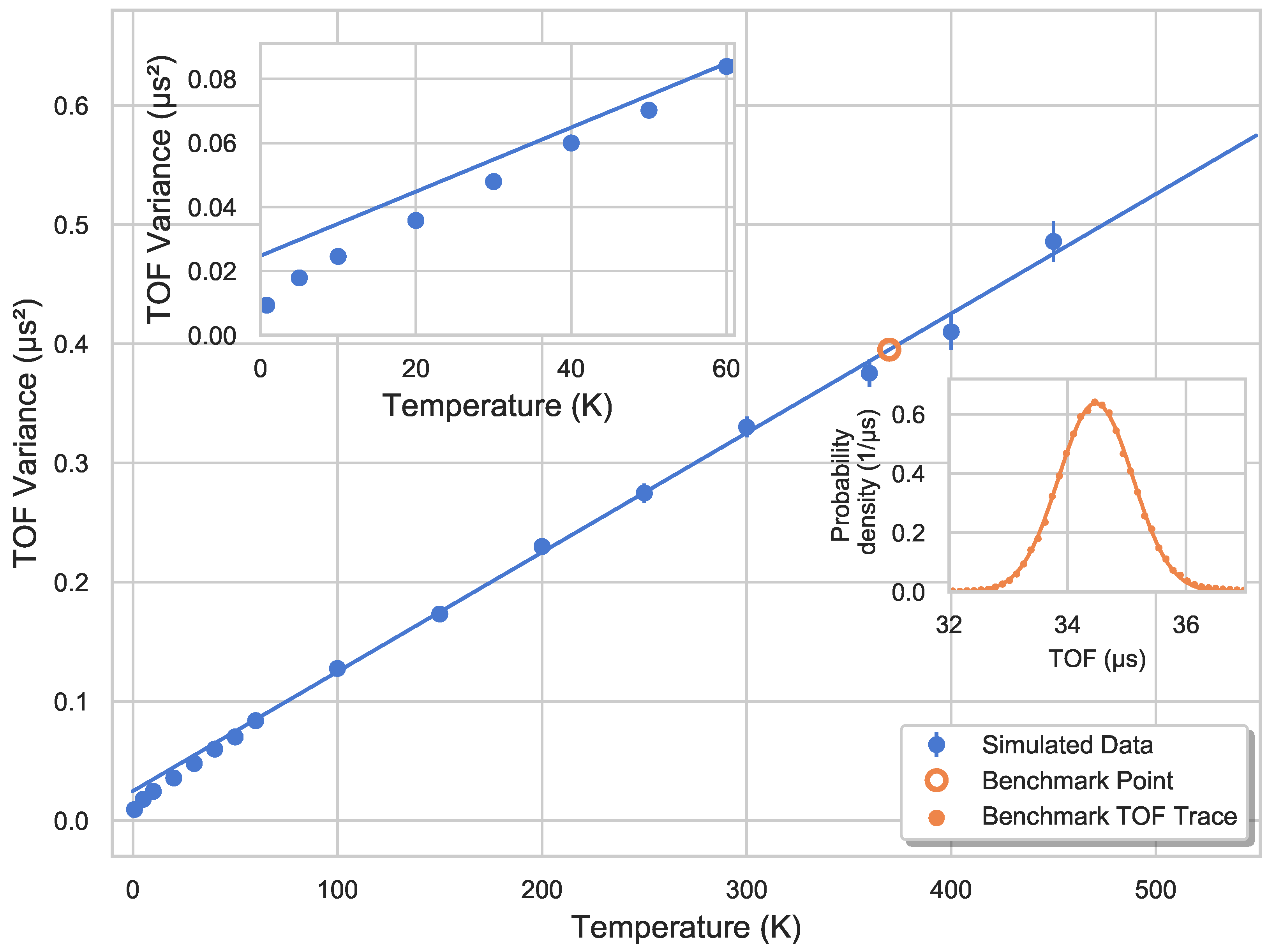
5.4. Correlation between Ions’ TOF Distribution and Their Translational Temperature

To model the extraction of the ions from the trap onto the detector, the ions are initially placed in the extraction potential of the trap at randomized initial positions and velocities. The velocity vectors are randomly sampled from a Maxwell–Boltzmann distribution at a given temperature. The ion’s position, though randomly sampled, is weighted with the simulated trapping potential, and expected ion distribution is calculated as ${\rho }_{\mathrm{ion}}\sim \exp (-\frac{V_{\mathrm{tot}}}{k_{\mathrm{B}}T})$. It is imperative to account for the simulated potential so as to accurately describe the appearance of pockets, i.e., regions of global maxima in the ion density distribution. Figure 8a shows a cut of the radial ion distribution at the axial local potential minimum (trap center) at 373 $\mathrm{K}$, while Figure 8b shows the same at 30 $\mathrm{K}$. At higher temperatures, the ion distribution is very homogeneous, but the effect of local potential minima becomes particularly pronounced at lower temperatures. The origin of these pockets lies in the symmetry-breaking of the potential, as reported in [32]. Here, the axial and vertical shielding electrodes have a strong influence in the trap center, thus leading to symmetry-breaking in the trap. This results in the two pockets, as the potential landscape is strongly dominated by the two pairs of shielding electrodes. The depth of the pockets is calculated from the energy of ions E via the relation $T=\frac{2E}{k_{\mathrm{B}}}$ to ∼60 $\mathrm{K}$. As previously mentioned, the initial positions and velocities of the ions are randomly sampled, prior to the extraction from the trap. The arrival time of the ions is then binned and subsequently represented by a Gaussian fit.

The expectation for the relationship between the variance of the ions’ TOF distribution and their temperature is a linear function. This assumption is based on the following considerations: Firstly, the TOF spread is primarily dominated by the velocity vectors along the main axis, pointing towards or opposite to the detector. The TOF spectrometer was adjusted to create a symmetric ion distribution via the axial shielding plates, as described in Section 3. The axial velocity spread is described by a Gaussian distribution with ${\sigma }_v^2\propto k_{\mathrm{B}}T$. Secondly, the axial spatial distribution is governed by the harmonic potential defined via a Gaussian distribution, where ${\sigma }_s^2\propto k_{\mathrm{B}}T$ holds valid again. Lastly, the extraction potential is well-approximated via sequential regions of linear acceleration. Thus, the axial velocity distribution of the ions can be linearly mapped onto the ions’ time of flight to the detector. In agreement with this expected behavior, a linear relationship between the variance, i.e., ${\sigma }^2$, of ions’ TOF distribution and their translational temperature is seen in Figure 9.

It is important to note that for temperatures lower than 60 $\mathrm{K}$, a deviation from the initial linear slope is seen. This can be attributed to the aforementioned occurrence of pockets in this temperature regime. The ions get trapped locally in these pockets which exhibit a more quadrupole-like character. During the extraction, this causes the radial velocity component of the ions pointing radially outwards to rapidly turn around, thus decreasing the time spent in the trap and hence, the TOF spread.

Using the time-of-flight (TOF) trace corresponding to the tomography from Figure 6, and the linear fit for temperatures above 60 $\mathrm{K}$ in Figure 9, one can calculate the temperature of the “benchmark measurement” as 370(12) $\mathrm{K}$. This is in line with the predicted value by the Monte-Carlo simulations. Since the tomography measurements are time-consuming, the calibration between the TOF variance and temperature of the ion ensemble provides a fast and reliable thermometry method to determine external or translational temperature of the ions trapped in a rf trap.

6. Conclusions

In this work, we presented a thermometry technique that uses the linear relationship between the motional temperature of an ensemble of ions trapped in a multipole trap and the variance of the time-of-flight distribution of the extracted ions. This technique provides a fast and reliable method to determine the energy distribution of, in principle, any ionic species confined in an ion trap, and can be used to measure the external temperature ranging from hundreds of Kelvin down to a few Kelvin. In our study, a deviation of the linear behavior was observed for lower temperatures. This is attributed to the existence of multiple potential minima in the trapping potential. These minima become more prominent at lower temperatures and were included in our model to obtain an accurate temperature calibration curve in the Kelvin range for our thermometry method. Additionally, the simulation of the trapping potential was modified to account for surface charge accumulation, thus increasing the accuracy of our model and allowing us to simulate the spatial distribution of the ion ensemble in the trap. This altered potential was determined by using an axial tomography measurement from our trap as well as a Monte-Carlo simulation, which predicted the energy distribution of ions colliding with room-temperature helium buffer gas. We showed that our octupole radio-frequency wire trap can create, with sufficiently higher voltage, nearly the same effective potential as the corresponding ideal hyperbolic or cylindrical rod trap. Further, a Monte-Carlo simulation shows that, after interaction with a room temperature helium buffer gas, the ions thermalize to the same final energy distribution in all the three trap types. A temperature higher than that of the buffer gas is obtained for all simulated traps attributed to the rf micromotion heating. These findings support that a wire trap with its superior optical access, in comparison to a trap utilizing thicker rods, is an ideal instrument for a hybrid trap and comes at little to no disadvantages. The optical access facilitates the laser cooling of rubidium atoms present in the chamber in order to create a dense atomic cloud and overlap it with the trapped ensemble of hydroxyl anions. With the flexibility to trap and characterize any ionic species in the setup, this system provides an excellent platform to study diverse atom–ion interactions.

References

1. Schuessler, H.A.; Holder, C.H.; Chun-Sing, O. Orbiting charge-transfer cross sections between He+ ions and cesium atoms at near-thermal ion-atom energies. Phys. Rev. A 1983, 28, 1817–1820. [Google Scholar] [CrossRef]
2. Côté, R. From Classical Mobility to Hopping Conductivity: Charge Hopping in an Ultracold Gas. Phys. Rev. Lett. 2000, 85, 5316–5319. [Google Scholar] [CrossRef] [PubMed]
3. Balakrishnan, N.; Dalgarno, A. Chemistry at Ultracold Temperatures. Chem. Phys. Lett. 2001, 341, 652–656. [Google Scholar] [CrossRef]
4. Rellergert, W.G.; Sullivan, S.T.; Kotochigova, S.; Petrov, A.; Chen, K.; Schowalter, S.J.; Hudson, E.R. Measurement of a Large Chemical Reaction Rate between Ultracold Closed-Shell 40Ca Atoms and Open-Shell 174Yb+ Ions Held in a Hybrid Atom-Ion Trap. Phys. Rev. Lett. 2011, 107, 243201. [Google Scholar] [CrossRef] [PubMed] [Green Version]
5. Willitsch, S. Coulomb-crystallised molecular ions in traps: Methods, applications, prospects. Int. Rev. Phys. Chem. 2012, 31, 175–199. [Google Scholar] [CrossRef]
6. Ravi, K.; Lee, S.; Sharma, A.; Werth, G.; Rangwala, S.A. Cooling and stabilization by collisions in a mixed ion-atom system. Nat. Commun. 2012, 3, 1126. [Google Scholar] [CrossRef] [Green Version]
7. Ratschbacher, L.; Zipkes, C.; Sias, C.; Köhl, M. Controlling chemical reactions of a single particle. Nat. Phys. 2012, 8, 649–652. [Google Scholar] [CrossRef]
8. Puri, P.; Mills, M.; Simbotin, I.; Montgomery, J.A.; Côté, R.; Schneider, C.; Suits, A.G.; Hudson, E.R. Reaction blockading in a reaction between an excited atom and a charged molecule at low collision energy. Nat. Chem. 2019, 11, 615–621. [Google Scholar] [CrossRef] [Green Version]
9. Dalgarno, A.; Rudge, M.R.H. Cooling of Interstellar Gas. Astrophys. J. 1964, 140, 800. [Google Scholar] [CrossRef]
10. Stancil, P.C.; Lepp, S.; Dalgarno, A. The lithium chemistry of the early Universe. Astrophys. J. 1996, 458, 401. [Google Scholar] [CrossRef]
11. Steigman, G. Charge transfer reactions in multiply charged ion-atom collisions. Astrophys. J. 1975, 199, 642–646. [Google Scholar] [CrossRef]
12. Vuitton, V.; Yelle, R.; McEwan, M. Ion chemistry and N-containing molecules in Titan’s upper atmosphere. Icarus 2007, 191, 722–742. [Google Scholar] [CrossRef]
13. Snow, T.P.; Bierbaum, V.M. Ion Chemistry in the Interstellar Medium. Ann. Rev. Anal. Chem. 2008, 1, 229–259. [Google Scholar] [CrossRef] [PubMed]
14. Vuitton, V.; Lavvas, P.; Yelle, R.; Galand, M.; Wellbrock, A.; Lewis, G.; Coates, A.; Wahlund, J.E. Negative ion chemistry in Titan’s upper atmosphere. Planet. Space Sci. 2009, 57, 1558–1572. [Google Scholar] [CrossRef]
15. Reddy, V.S.; Ghanta, S.; Mahapatra, S. First Principles Quantum Dynamical Investigation Provides Evidence for the Role of Polycyclic Aromatic Hydrocarbon Radical Cations in Interstellar Physics. Phys. Rev. Lett. 2010, 104, 111102. [Google Scholar] [CrossRef]
16. Bohringer, H.; Glebe, W.; Arnold, F. Temperature dependence of the mobility and association rate coefficient of He+ions in He from 30–350K. J. Phys. B At. Mol. Phys. 1983, 16, 2619–2626. [Google Scholar] [CrossRef]
17. Eppink, A.T.J.B.; Parker, D.H. Velocity map imaging of ions and electrons using electrostatic lenses: Application in photoelectron and photofragment ion imaging of molecular oxygen. Rev. Sci. Instrum. 1997, 68, 3477–3484. [Google Scholar] [CrossRef]
18. Neuhauser, W.; Hohenstatt, M.; Toschek, P.E.; Dehmelt, H. Localized visible Ba+ mono-ion oscillator. Phys. Rev. A 1980, 22, 1137–1140. [Google Scholar] [CrossRef]
19. Bergquist, J.C.; Wineland, D.J.; Itano, W.M.; Hemmati, H.; Daniel, H.U.; Leuchs, G. Energy and Radiative Lifetime of the 5d96s22 D 5 2 State in Hg II by Doppler-Free Two-Photon Laser Spectroscopy. Phys. Rev. Lett. 1985, 55, 1567–1570. [Google Scholar] [CrossRef]
20. Segall, J.; Lavi, R.; Wen, Y.; Wittig, C. Acetylene carbon-hydrogen bond dissociation energy using 193.3-nm photolysis and sub-Doppler resolution hydrogen-atom spectroscopy: 127 .+-. 1.5 kcal mol−1. J. Phys. Chem. 1989, 93, 7287–7289. [Google Scholar] [CrossRef]
21. Kinugawa, T.; Arikawa, T. Three-dimensional velocity analysis combining ion imaging with Doppler spectroscopy: Application to photodissociation of HBr at 243 nm. J. Chem. Phys. 1992, 96, 4801–4804. [Google Scholar] [CrossRef] [Green Version]
22. Schlemmer, S.; Kuhn, T.; Lescop, E.; Gerlich, D. Laser excited N2+ in a 22-pole ion trap:: Experimental studies of rotational relaxation processes. Int. J. Mass Spectrom. 1999, 185–187, 589–602. [Google Scholar] [CrossRef]
23. Glosík, J.; Hlavenka, P.; Plašil, R.; Windisch, F.; Gerlich, D.; Wolf, A.; Kreckel, H. Action spectroscopy of and D2H+ using overtone excitation. Philos. Trans. R. Soc. A Math. Phys. Eng. Sci. 2006, 364, 2931–2942. [Google Scholar] [CrossRef] [PubMed]
24. Otto, R.; von Zastrow, A.; Best, T.; Wester, R. Internal state thermometry of cold trapped molecular anions. Phys. Chem. Chem. Phys. 2013, 15, 612–618. [Google Scholar] [CrossRef] [PubMed] [Green Version]
25. Lakhmanskaya, O.; Simpson, M.; Wester, R. Vibrational overtone spectroscopy of cold trapped hydroxyl anions. Phys. Rev. A 2020, in press. [Google Scholar] [CrossRef]
26. Deiglmayr, J.; Göritz, A.; Best, T.; Weidemüller, M.; Wester, R. Reactive collisions of trapped anions with ultracold atoms. Phys. Rev. A 2012, 86, 043438. [Google Scholar] [CrossRef] [Green Version]
27. Trippel, S.; Mikosch, J.; Berhane, R.; Otto, R.; Weidemüller, M.; Wester, R. Photodetachment of cold OH in a multipole ion trap. Phys. Rev. Lett. 2006, 97, 193003. [Google Scholar] [CrossRef] [Green Version]
28. Hlavenka, P.; Otto, R.; Trippel, S.; Mikosch, J.; Weidemüller, M.; Wester, R. Absolute photodetachment cross section measurements of the O and OH anion. J. Chem. Phys. 2009, 130, 061105. [Google Scholar] [CrossRef] [Green Version]
29. Osborn, D.L.; Leahy, D.J.; Cyr, D.R.; Neumark, D.M. Photodissociation spectroscopy and dynamics of the N2O2 anion. J. Chem. Phys. 1996, 104, 5026–5039. [Google Scholar] [CrossRef]
30. Höltkemeier, B.; Glässel, J.; López-Carrera, H.; Weidemüller, M. A dense gas of laser-cooled atoms for hybrid atom-ion trapping. Appl. Phys. B Lasers Opt. 2017, 123, 51. [Google Scholar] [CrossRef]
31. Nadarajah, S. A generalized normal distribution. J. Appl. Stat. 2005, 32, 685–694. [Google Scholar] [CrossRef]
32. Otto, R.; Hlavenka, P.; Trippel, S.; Mikosch, J.; Singer, K.; Weidemüller, M.; Wester, R. How can a 22-pole ion trap exhibit ten local minima in the effective potential? J. Phys. B At. Mol. Opt. Phys. 2009, 42, 154007. [Google Scholar] [CrossRef]
33. Okada, K.; Yasuda, K.; Takayanagi, T.; Wada, M.; Schuessler, H.A.; Ohtani, S. Crystallization of Ca+ ions in a linear rf octupole ion trap. Phys. Rev. A 2007, 75, 033409. [Google Scholar] [CrossRef] [Green Version]
34. Wester, R. Radiofrequency multipole traps: Tools for spectroscopy and dynamics of cold molecular ions. J. Phys. B At. Mol. Opt. Phys. 2009, 42, 154001. [Google Scholar] [CrossRef]
35. Gerlich, D. Inhomogeneous RF Fields: A Versatile Tool for the Study of Processes with Slow Ions. In Advances in Chemical Physics; John Wiley & Sons, Ltd.: Hoboken, NJ, USA, 2007; pp. 1–176. [Google Scholar] [CrossRef]
36. Ter Haar, D. (Ed.) The Maxwell—Boltzmann Distribution. In Elements of Statistical Mechanics, 3rd ed.; Butterworth-Heinemann: Oxford, UK, 1995; Chapter 2; pp. 36–58. [Google Scholar] [CrossRef]
37. Asvany, O.; Schlemmer, S. Numerical simulations of kinetic ion temperature in a cryogenic linear multipole trap. Int. J. Mass Spectrom. 2009, 279, 147–155. [Google Scholar] [CrossRef]
38. Tsallis, C. Possible generalization of Boltzmann-Gibbs statistics. J. Stat. Phys. 1988, 52, 479–487. [Google Scholar] [CrossRef]
39. Tsallis, C.; Mendes, R.; Plastino, A. The role of constraints within generalized nonextensive statistics. Phys. A Stat. Mech. Appl. 1998, 261, 534–554. [Google Scholar] [CrossRef]
40. Höltkemeier, B.; Weckesser, P.; López-Carrera, H.; Weidemüller, M. Dynamics of a single trapped ion immersed in a buffer gas. Phys. Rev. A 2016, 94, 062703. [Google Scholar] [CrossRef] [Green Version]
41. Höltkemeier, B.; Weckesser, P.; López-Carrera, H.; Weidemüller, M. Buffer-Gas Cooling of a Single Ion in a Multipole Radio Frequency Trap Beyond the Critical Mass Ratio. Phys. Rev. Lett. 2016, 116, 233003. [Google Scholar] [CrossRef] [Green Version]
42. Rouse, I.; Willitsch, S. Superstatistical Energy Distributions of an Ion in an Ultracold Buffer Gas. Phys. Rev. Lett. 2017, 118, 143401. [Google Scholar] [CrossRef] [Green Version]
43. COMSOL Multiphysics, Version 5.4. Available online: https://www.comsol.com/ (accessed on 16 June 2020).
44. Friedman, M.H.; Yergey, A.L.; Campana, J.E. Fundamentals of ion motion in electric radio-frequency multipole fields. J. Phys. E Sci. Instrum. 1982, 15, 53–56. [Google Scholar] [CrossRef]
Figure 1. Schematic representation of the Hybrid Atom–Ion Trap (HAI-trap). The ions are produced via a plasma discharge in a pulsed molecular beam and are then guided towards a Wiley–McLaren time-of-flight spectrometer, where the ions are separated according to their mass-to-charge ratio. The ion beam is then guided into the trap, and the entrance endcap is switched to mass-select the desired species. Subsequently, the ions can be overlapped with a cloud of laser-cooled atoms to study atom–ion interactions, or a detachment laser beam can be shone onto the ion cloud for photodetachment tomography. Finally, the ions are extracted via the hollow endcap onto a detector that records the ions’ arrival time.
Applsci 10 05264 g001
Figure 2. Description of the ion trap. (a) A 3D model of the ion trap is shown with an illustration of the radio frequency (rf) trap wires, endcap electrodes, and shielding plates used in the setup. (b) A qualitative description of the electric potential as a function of the position along the trap’s main axis during three different stages. Firstly, the loading of ions from the source into the trap. Secondly, the axial confinement of ions. Finally, the unloading of ions from the trap to be further extracted onto the detector.
Applsci 10 05264 g002
Figure 3. Comparison between different multipole traps. (a) True size relations between hyperbolic rods, ideal cylindrical rods, and cylindrical wires are represented. The distance of a hyperbolic rod from the trap center is r 0 = 2.25 mm, the diameter of an ideal cylindrical rod is 2 ρ = 1.5 mm and the wire diameter is d = 100   μ m . The wires are placed concentrically with the ideal cylindrical rods and are located 3 mm from the trap center. (b) The effective potential created by hyperbolic rods is shown along with that obtained from a rod and a wire trap with their voltages matched to the same average potential as in the hyperbolic case. It can be seen that the hyperbolic trap potential exhibits true azimuthal angle independence, while distinct maxima/minima in the potential for traps with cylindrical rods or wires can be observed. Additionally, the modulations in a wire trap have a higher amplitude than those in a rod trap. For instance, the amplitude of fluctuations in a rod trap at 0.87 · r 0 is already attained by a wire trap at 0.81 · r 0 .
Applsci 10 05264 g003
Figure 4. Simulated energy distribution of ions after collisions with helium buffer gas at 293 K for different trap configurations are shown. For traps with hyperbolic rods, cylindrical rods, and wires, the temperature obtained from the distributions are all 366 K , using Equation (3). On comparison with an analytical Maxwell–Boltzmann distribution at 366 K (black dashed line), it can be seen that the distribution is not perfectly thermal.
Applsci 10 05264 g004
Figure 5. Simulated energy distribution of ions thermalized with a 293 K helium buffer gas in the HAI-trap potential landscape. The energy of the ions is characterized via a Tsallis with T = 313 ( 2 )   K and q = 1.070 ( 2 ) as well as a Maxwell distribution with T = 359 ( 3 )   K . It can be seen that the Maxwell fit overestimates the relative amount of low-energy to mid-energy and underestimates the high-energy tails which are then better represented via a Tsallis distribution (as shown in graph inset).
Applsci 10 05264 g005
Figure 6. Column density profile as a function of the axial laser position along the cylindrical axis of the trap. Each point was derived by fitting a first-order exponential decay to the ion signal for multiple interaction times with a far-threshold laser beam. The standard deviation of the fits are presented by the error bars. The measured density distribution is compared with the simulated potential which accounts for surface charges. Equations (5) and (6) are used to derive a density distribution from this potential using the simulated energy distribution from Figure 5. The probability density curves shown here are normalized to 1.
Applsci 10 05264 g006
Figure 7. Characterization of surface charge accumulation on PCBs. The surface charge distribution is defined such that the tomography measurements for 80 V endcap voltage matches the simulated ion distribution at a temperature of 373 K . Once the charges are fixed, the modified potential is used to obtain the ion distribution for a configuration with 40 V endcap voltage, which matches the measured ion density distribution for the chosen endcap voltage.
Applsci 10 05264 g007
Figure 8. Heatmap representation for the density distribution of ions in the trap. (a) Homogenoues ion density distribution at 373 K . (b) Ion density distribution at 30 K exhibiting regions of global maxima called “pockets”. The depth of the pockets is calculated from the energy of ions E via the relation T = 2 E k B to ∼60 K . The axes used are corresponding to the coordinates shown in Figure 2.
Applsci 10 05264 g008
Figure 9. The variance of the TOF distribution, i.e., σ 2 , plotted as a function of the initial temperature of the ions in the trap before extraction onto the detector. The change in the linear slope can be seen in the left inset. It is interpreted as a consequence of the pockets arising at a temperature regime of about 60 K . Furthermore, the temperature from the corresponding TOF trace of the tomography measurements is derived to be 370 K , which is consistent with the Monte-Carlo simulations’ prediction. This TOF trace is shown in the right inset along with the Gaussian fit representing the distribution.
Applsci 10 05264 g009