A Workspace Visualization Method for a Multijoint Industrial Robot Based on the 3D-Printing Layering Concept

Abstract

The workspace of a robot provides the necessary constraint information for path planning and reliable control of the robot. In this paper, a workspace visualization method for a multijoint industrial robot is proposed to obtain a detailed workspace by introducing the 3D-printing layering concept. Firstly, all possible joint-angle groups of one pose in the joints’ ranges are calculated in detail according to the POE (product of exponential) theory-based forward-kinematics expressions of the multijoint industrial robot. Secondly, a multisolution selection method based on the key degree of the joint is proposed to select the appropriate joint-angle groups. The key degrees of all joints and their key order are obtained according to the sensitivity expressions of all joint angles, calculated from the Jacobian matrix of the robot. One principle based on the smallest differences of the nominal angle is established to select the possible solutions for one joint from the possible solutions for the joint with the smaller key order. The possible solutions for the joint with the highest key order are the appropriate joint-angle group. Thirdly, a workspace visualization method based on the layering concept of 3D printing is presented to obtain a detailed workspace for a multijoint industrial robot. The boundary formula of each layer is derived by forward kinematics, which is expressed as a circle or a ring. The maximum and minimum values of the radius are obtained according to the travel range of the joint angles. The height limitations of all layers are obtained with forward kinematics. A workspace boundary-extraction method is presented to obtain the array of path points of the boundary at each layer. The proposed postprocessing method is used to generate the joint-angle code of each layer for direct 3D printing. Finally, the effectiveness of the multisolution selection method and the workspace visualization method were verified by simulation and experiment.

1. Introduction

Industrial robots play an important role in manufacturing as manufacturing automation and intelligence continuously improve. The industrial robot industry is an important indicator of a country′s manufacturing level and technology level. Industrial robots are widely used in different fields, such as automobile manufacturing, electrical and electronics, and aerospace. In addition, industrial robots are core pieces of equipment for the industrial intelligent manufacturing. The workspace of a robot is an important index of the flexibility of the robot. It provides the necessary constraint information for the path planning and control of the robot. It has important significance in the structural design and path planning.

Kinematics represent the relationship between the position and the pose of the end-effector and the joint variables. This lays the basis for the workspace of the multijoint industrial robots. The Denavit–Hartenberg (D-H) parametric method is a standard method of modeling [1,2,3]. Cumulative errors may be increased with the increased degrees of freedom when using this method. POE (product of exponential) theory is another option for kinematics modeling [4,5,6,7]. An et al. gave a generalized solution of a kinematics problem based on POE in order to analyze the kinematics problems of serial robots [8]. Ayiz et al. used POE theory to solve kinematics problems of industrial robots [9]. POE theory allows global description of rigid body motion and greatly simplifies the analysis of mechanisms. For inverse kinematics, the common methods are the algebraic method, geometric method, and numerical method. Yahya et al. proposed a geometric method to find the optimal solution of the inverse kinematics of redundant or hyperredundant robots from infinite solutions [10]. Ananthanarayanan et al. obtained the inverse kinematics solution by using iteration methods with the initial value of the analytical solution [11]. Modern intelligent algorithms are also widely used to solve the inverse kinematics of robots with complex structures. Baheshti et al. used the adaptive fuzzy logic method to determine the inverse kinematics solution of a 3-DOF (degree of freedom) planar robot [12]. Ayyıldız et al. obtained the solution of an inverse kinematics equation by using four different optimization algorithms [13]. These methods can produce accurate inverse kinematics solutions, but they need a lot of training. The inverse kinematics solution of robots is a multisolution problem. The criterion of shortest travel is generally adopted to select the appropriate solution. Wang et al. proposed a criterion of weighted shortest travel, and selected the appropriate solution by finding the minimum value of weighted Euclidean distance [14]. Liu et al. divided the result of inverse solution with the geometric attitude of the robot to facilitate selection [15].

The determination of the workspace boundary is generally an intermediate but critical step in analyzing multijoint industrial robots [16]. Traditionally, the workspace boundaries of multijoint industrial robots are usually expressed as numerical curves on the boundaries or analytical formulas of a certain kind of robot. Abdel-malek et al. used differential geometry and topology methods to obtain general formulas for the workspace recognition and visualization using the manifold layering method [17]. Wang et al. used the surface envelope overlay (SEO) method to identify and visualize the robot workspace [16]. Graphic methods are another way to find workspace boundaries [18]. Gan et al. took advantage of the arm length of a robot and the angle ranges of its joints to obtain section screenshots of the robot’s workspace on the xz plane via the geometric drawing method [19]. Liu et al. discussed the geometric description of a robot’s workspace and presented the design results of a delta robot for a given workspace [20]. This method is more intuitive, but it is not suitable for robots with more than 3 degrees of freedom. Most of the analysis methods try to extract boundary information from singular points of robots by analyzing the characteristics of the singular points. Based on this theorem, several analytical criteria for determining the workspaces boundaries were derived [21]. Kohli et al. analyzed a workspace and subspace by polynomial criterion and Jacobian matrix, respectively [22,23]. Yang et al. described singular behavior with the row rank defect of the Jacobian matrix and presented the boundary subsurface of the envelope of a workspace using the perturbation method by dividing the singular surface into several subsurfaces [24].

Most numerical methods of singularities or bounds are mapped by grids. All grid-based methods produce an approximate boundary, and the accuracy depends on the size of the grid. The Monte Carlo method is commonly used to generate sample points in a grid in order to identify the grid points near the workspace boundary via the statistical method, which bypasses the necessity of tightness. Cao et al. generated random values of the joint vector data by increasing the probability of the joint vector at the workspace boundary with the upper limit and lower limit of the joint angles [25]. Peidro et al. used the classical Monte Carlo method to generate an inaccurate workspace and used a Gaussian distribution to encrypt and extend the workspace until the boundary of the workspace was reached [26]. Liu et al. added random points locally at the boundary points of each layer in order to generate a clear workspace boundary [27]. However, this method cannot exclude the identification of false holes in the workspace. The layering concept in 3D printing can be introduced to obtain expressions of workspace boundaries, which makes the visualization of the workspace feasible.

In addition, interval-analysis-based methods have been used to analyze workspaces. Interval analysis can be used to evaluate the constraints, and branch-and-prune techniques used to characterize the constraint workspace. This is the basis of prescribed bounded velocity and force transmission factors. Merlet et al. proposed an interval-analysis-based approach to determine almost all the geometries of a simplified Gough platform for which the workspace included an arbitrary set of poses [28]. Chablat et al. used interval analysis to compute a dextrous workspace as well as the largest cube enclosed in this workspace [29]. Kaloorazi et al. proposed a systematic algorithm based on the interval-analysis concept in order to find the maximal singularity-free circle or sphere within the workspace of parallel mechanisms [30]. Viegas et al. used interval analysis to evaluate several performance indexes of parallel kinematic machine design [31]. However, interval-analysis-based methods are mostly used to analyze the workspace of parallel mechanisms.

This paper proposes a new workspace visualization method based on a 3D-printing layering concept in order to obtain and visualize the workspace accurately. At first, all possible solutions of joint angles are obtained in detail based on the forward kinematics and inverse kinematics of a multijoint industrial robot. Next, one multisolution selection method is proposed according to the sensitivity-based key degree of the joints to select the appropriate solutions. Next, a 3D-printing layering concept is introduced to establish one workspace visualization method. The forward kinematics can help to establish the boundary formula of each layer and obtain the limitation of the height of the workspace. The multisolution selection method can help to obtain the joint angles of each layer, which also can be used to print the workspace.

The remains of the paper are organized as follows: In Section 2, the kinematics model of a multijoint industrial robot based on POE theory is established, and all possible joint-angle groups of one pose in the joint range are presented in detail. In Section 3, a multisolution selection method based on the key degree of joints is proposed. Section 4 presents a workspace visualization method based on a 3D-printing layering concept. Section 5 describes the validation of the simulation and experiments that were carried out.

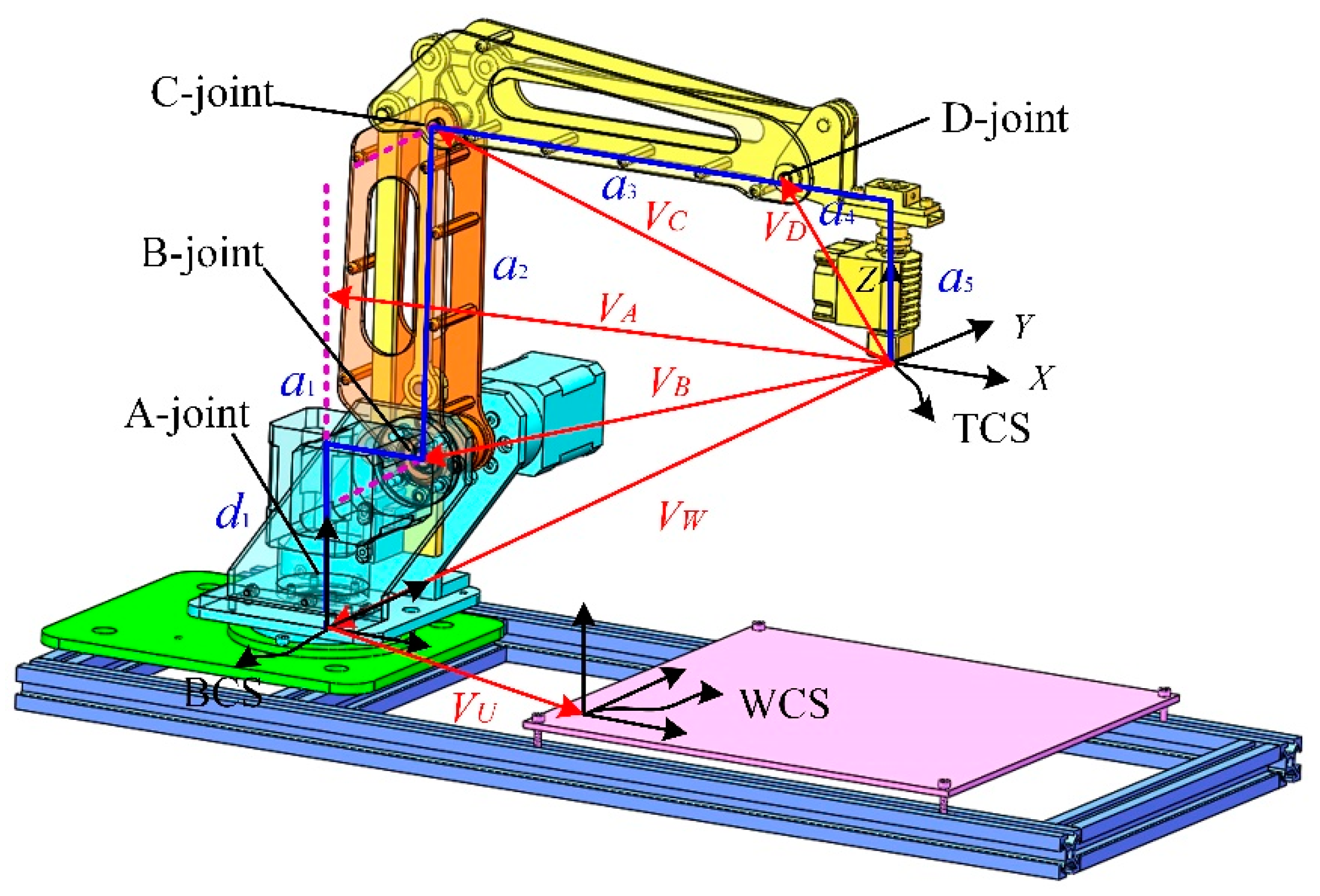
2. Kinematic Model of a Multijoint Industrial Robot

2.1. Forward Kinematics Based on POE Theory

Figure 1 shows the structure and structural parameters of a multijoint industrial robot, and Figure 2 shows the kinematic chain. BCS is the base coordinate system, TCS is the tool coordinate system, and WCS is the workpiece coordinate system. The structural parameters V_A, V_B, V_C, V_D, and V_W represent the positions of the A-joint, B-joint, C-joint, D-joint, and the base relative to the end-effector, respectively. V_U represents the position of the workpiece relative to the base. They were represented as

$$\{\begin{array}{l}{\mathrm{V}}_{\mathrm{A}}={\left[{\mathrm{A}}_{\mathrm{x}},{\mathrm{A}}_{\mathrm{y}},0\right]}^{\mathrm{T}}={\left[-\left({\mathrm{a}}_1+{\mathrm{a}}_3+{\mathrm{a}}_4\right),0,0\right]}^{\mathrm{T}}\\ {\mathrm{V}}_{\mathrm{B}}={\left[{\mathrm{B}}_{\mathrm{x}},0,{\mathrm{B}}_{\mathrm{z}}\right]}^{\mathrm{T}}={\left[-\left({\mathrm{a}}_3+{\mathrm{a}}_4\right),0,{\mathrm{a}}_5-{\mathrm{a}}_2\right]}^{\mathrm{T}}\\ {\mathrm{V}}_{\mathrm{C}}={\left[{\mathrm{C}}_{\mathrm{x}},0,{\mathrm{C}}_{\mathrm{z}}\right]}^{\mathrm{T}}={\left[-\left({\mathrm{a}}_3+{\mathrm{a}}_4\right),0,{\mathrm{a}}_5\right]}^{\mathrm{T}}\\ {\mathrm{V}}_{\mathrm{D}}={\left[{\mathrm{D}}_{\mathrm{x}},0,{\mathrm{D}}_{\mathrm{z}}\right]}^{\mathrm{T}}={\left[-{\mathrm{a}}_4,0,{\mathrm{a}}_5\right]}^{\mathrm{T}}\\ {\mathrm{V}}_{\mathrm{W}}={\left[{\mathrm{W}}_{\mathrm{x}},{\mathrm{W}}_{\mathrm{y}},{\mathrm{W}}_{\mathrm{z}}\right]}^{\mathrm{T}}={\left[-\left({\mathrm{a}}_1+{\mathrm{a}}_3+{\mathrm{a}}_4\right),0,{\mathrm{a}}_5-{\mathrm{a}}_2-{\mathrm{d}}_1\right]}^{\mathrm{T}}\\ {\mathrm{V}}_{\mathrm{U}}={\left[{\mathrm{U}}_{\mathrm{x}},{\mathrm{U}}_{\mathrm{y}},{\mathrm{U}}_{\mathrm{z}}\right]}^{\mathrm{T}}\end{array}$$

(1)

The clear geometric meaning of POE theory makes it an effective tool for kinematic modeling. One twist can represent the motion of one rigid body. The twist coordinates can be written as

$$\mathsf{\xi }={\left[{\mathsf{\omega }}^{\mathrm{T}},{\mathsf{\nu }}^{\mathrm{T}}\right]}^{\mathrm{T}}$$

(2)

where ω is the unit vector of the rotational axis; ν is the linear velocity of the rotational motion; vector ν can be obtained as ν = p × ω; p is the position vector in the base for a point fixed on the axis; and the exponential matrix of the twist is represented as

$$\mathrm{g}={\mathrm{e}}^{\mathsf{\xi }\mathsf{\theta }}=\{\begin{array}{ll}\left[\begin{array}{cc}{\mathrm{e}}^{\mathsf{\omega }\mathsf{\theta }}& \left(\mathrm{I}-{\mathrm{e}}^{\mathsf{\omega }\mathsf{\theta }}\right)\left(\mathsf{\omega }\times \mathsf{\nu }\right)+\mathsf{\omega }{\mathsf{\omega }}^{\mathrm{T}}\mathsf{\nu }\mathsf{\theta }\\ 0& 1\end{array}\right]& \mathrm{i}\mathrm{f} \mathsf{\omega }\ne 0\\ \left[\begin{array}{cc}\mathrm{I}& \mathsf{\nu }\mathsf{\theta }\\ 0& 1\end{array}\right]& \mathrm{i}\mathrm{f} \mathsf{\omega }=0\end{array}$$

(3)

where e^ωθ can be calculated by following the formula

$${\mathrm{e}}^{\mathsf{\omega }\mathsf{\theta }}=\mathrm{I}+\mathsf{\omega }\sin \mathsf{\theta }+{\mathsf{\omega }}^2\left(1-\cos \mathsf{\theta }\right)$$

(4)

Using the POE formula, the forward kinematics of a multijoint industrial robot with n joints can be expressed as

$${\mathrm{g}}_{\mathrm{s}\mathrm{t}}\left(\mathsf{\theta }\right)={\mathrm{e}}^{{\mathsf{\xi }}_1{\mathsf{\theta }}_1}{\mathrm{e}}^{{\mathsf{\xi }}_2{\mathsf{\theta }}_2}\cdot \cdot \cdot {\mathrm{e}}^{{\mathsf{\xi }}_{\mathrm{n}}{\mathsf{\theta }}_{\mathrm{n}}}$$

(5)

In order to obtain the position of the print nozzle (the end-effector) relative to the workpiece, and solve the inverse kinematics conveniently, the base coordinate system was set as the global coordinate system. The obtained kinematic POE formula was translated to the workpiece coordinate system in order to obtain the position of the print nozzle relative to the workpiece. A multijoint industrial robot can be seen as one open chain from the base to the printing nozzle. As shown in Figure 2, the order of the open chain is base→A-joint→B-joint→C-joint→D-joint→printing nozzle. Point R_A is the intersection point of the rotation axis of the A-joint. The coordinates of R_A in BCS are R_A = −V_W + V_A. Point R_B is the intersection point of the rotation axis of the B-joint. The coordinates relative to BCS are R_B = −V_W + V_B. Point R_C is the intersection point of the rotation axis of the C-joint. The coordinates relative to BCS are R_C = −V_W + V_C. Point R_D is the intersection point of the rotation axis of the D-joint. The coordinates relative to BCS are R_D = −V_W + V_D. First, motion twists and exponential matrices of all axes were established according to the kinematic chain and POE theory. Unit twists of the A-joint, B-joint, C-joint, and D-joint were expressed as

$$\{\begin{array}{l}{\mathsf{\xi }}_1={\left[{\mathsf{\omega }}_1^{\mathrm{T}},{\left({\mathrm{p}}_1\times {\mathsf{\omega }}_1\right)}^{\mathrm{T}}\right]}^{\mathrm{T}}={\left[0,0,1,-{\mathrm{W}}_{\mathrm{y}},-\left({\mathrm{A}}_{\mathrm{x}}-{\mathrm{W}}_{\mathrm{x}}\right),0\right]}^{\mathrm{T}}\\ {\mathsf{\xi }}_2={\left[{\mathsf{\omega }}_2^{\mathrm{T}},{\left({\mathrm{p}}_2\times {\mathsf{\omega }}_2\right)}^{\mathrm{T}}\right]}^{\mathrm{T}}={\left[0,1,0,-\left({\mathrm{B}}_{\mathrm{z}}-{\mathrm{W}}_{\mathrm{z}}\right),0,{\mathrm{B}}_{\mathrm{x}}-{\mathrm{W}}_{\mathrm{x}}\right]}^{\mathrm{T}}\\ {\mathsf{\xi }}_3={\left[{\mathsf{\omega }}_3^{\mathrm{T}},{\left({\mathrm{p}}_3\times {\mathsf{\omega }}_3\right)}^{\mathrm{T}}\right]}^{\mathrm{T}}={\left[0,1,0,-\left({\mathrm{C}}_{\mathrm{z}}-{\mathrm{W}}_{\mathrm{z}}\right),0,{\mathrm{C}}_{\mathrm{x}}-{\mathrm{W}}_{\mathrm{x}}\right]}^{\mathrm{T}}\\ {\mathsf{\xi }}_4={\left[{\mathsf{\omega }}_4^{\mathrm{T}},{\left({\mathrm{p}}_4\times {\mathsf{\omega }}_4\right)}^{\mathrm{T}}\right]}^{\mathrm{T}}={\left[0,1,0,-\left({\mathrm{C}}_{\mathrm{z}}-{\mathrm{W}}_{\mathrm{z}}\right),0,{\mathrm{D}}_{\mathrm{x}}-{\mathrm{W}}_{\mathrm{x}}\right]}^{\mathrm{T}}\end{array}$$

(6)

According to the order of the open chain, the transformation matrix of a multijoint industrial robot can be obtained with the exponential matrix of each joint. The movements of all joints relative to their local zero positions are positive relative to the global coordinate system (BCS). The POE formula of the tool relative to the base of the multijoint industrial robot was then expressed as

$${}_{\mathrm{t}}{}^{\mathrm{b}}\mathrm{T}={\mathrm{e}}^{{\mathsf{\xi }}_{\mathrm{b}}}\cdot {\mathrm{e}}^{{\mathsf{\xi }}_1\mathrm{\alpha }}\cdot {\mathrm{e}}^{{\mathsf{\xi }}_2\mathsf{\beta }}\cdot {\mathrm{e}}^{{\mathsf{\xi }}_3\mathsf{\gamma }}\cdot {\mathrm{e}}^{{\mathsf{\xi }}_4\mathrm{\delta }}\cdot {\mathrm{e}}^{{\mathsf{\xi }}_{\mathrm{t}}}=\left[\begin{array}{cccc}{\mathrm{n}}_{\mathrm{x}}& {\mathrm{o}}_{\mathrm{x}}& {\mathrm{a}}_{\mathrm{x}}& {\mathrm{P}}_{\mathrm{x}}^{\prime }\\ {\mathrm{n}}_{\mathrm{y}}& {\mathrm{o}}_{\mathrm{y}}& {\mathrm{a}}_{\mathrm{y}}& {\mathrm{P}}_{\mathrm{y}}^{\prime }\\ {\mathrm{n}}_{\mathrm{z}}& {\mathrm{o}}_{\mathrm{z}}& {\mathrm{a}}_{\mathrm{z}}& {\mathrm{P}}_{\mathrm{z}}^{\prime }\\ 0& 0& 0& 1\end{array}\right],$$

(7)

where ξ_b = ξ_t = [0,0,0,0,0,0] represents the twist of the base and the printing nozzle, respectively. The pose matrix is R = [n,o,a] and the position matrix is P = [P_x’,P_y’,P_z’]^T. However, it can be seen from Figure 1 that the fourth joint of the multijoint industrial robot modeled in this paper is a false joint. Due to this limitation of the mechanical structure, the end-effector is always parallel to the printing platform, meaning that δ = −β − γ can be obtained from the geometry, namely

$$\left[\begin{array}{c}{\mathrm{P}}_{\mathrm{x}}{}^{\prime }\\ {\mathrm{P}}_{\mathrm{y}}{}^{\prime }\\ {\mathrm{P}}_{\mathrm{z}}{}^{\prime }\end{array}\right]=\left[\begin{array}{c}\cos \mathrm{\alpha }\left[{\mathrm{a}}_3\cos \left(\mathsf{\beta }+\mathsf{\gamma }\right)+{\mathrm{a}}_2\cos \mathsf{\beta }+{\mathrm{a}}_1+{\mathrm{a}}_4\right]\\ \sin \mathrm{\alpha }\left[{\mathrm{a}}_3\cos \left(\mathsf{\beta }+\mathsf{\gamma }\right)+{\mathrm{a}}_2\cos \mathsf{\beta }+{\mathrm{a}}_1+{\mathrm{a}}_4\right]\\ {\mathrm{a}}_3\sin \left(\mathsf{\beta }+\mathsf{\gamma }\right)+{\mathrm{a}}_2\sin \mathsf{\beta }+{\mathrm{d}}_1-{\mathrm{a}}_5\end{array}\right]$$

(8)

According to Equation (3), the position and pose of the multijoint industrial robot can be obtained. The last three joints of the common six-joint industrial robots are concentrated on the wrist to indicate pose and the first three joints indicate the position. Due to the limitation of the mechanical structure of the robot modeled in this paper and the existing 3D-printing methods, only three joints were considered. Thus, the forward kinematics equations of the printing nozzle relative to the workpiece were expressed as

$$\{\begin{array}{l}{\mathrm{P}}_{\mathrm{x}}=\cos \alpha \left[{\mathrm{a}}_3\cos \left(\beta +\gamma \right)+{\mathrm{a}}_2\cos \beta +{\mathrm{a}}_1+{\mathrm{a}}_4\right]-{\mathrm{U}}_{\mathrm{x}}\\ {\mathrm{P}}_{\mathrm{y}}=\sin \alpha \left[{\mathrm{a}}_3\cos \left(\beta +\gamma \right)+{\mathrm{a}}_2\cos \beta +{\mathrm{a}}_1+{\mathrm{a}}_4\right]-{\mathrm{U}}_{\mathrm{y}}\\ {\mathrm{P}}_{\mathrm{z}}={\mathrm{a}}_3\sin \left(\beta +\gamma \right)+{\mathrm{a}}_2\sin \beta +{\mathrm{d}}_1-{\mathrm{a}}_5-{\mathrm{U}}_{\mathrm{z}}\end{array}$$

(9)

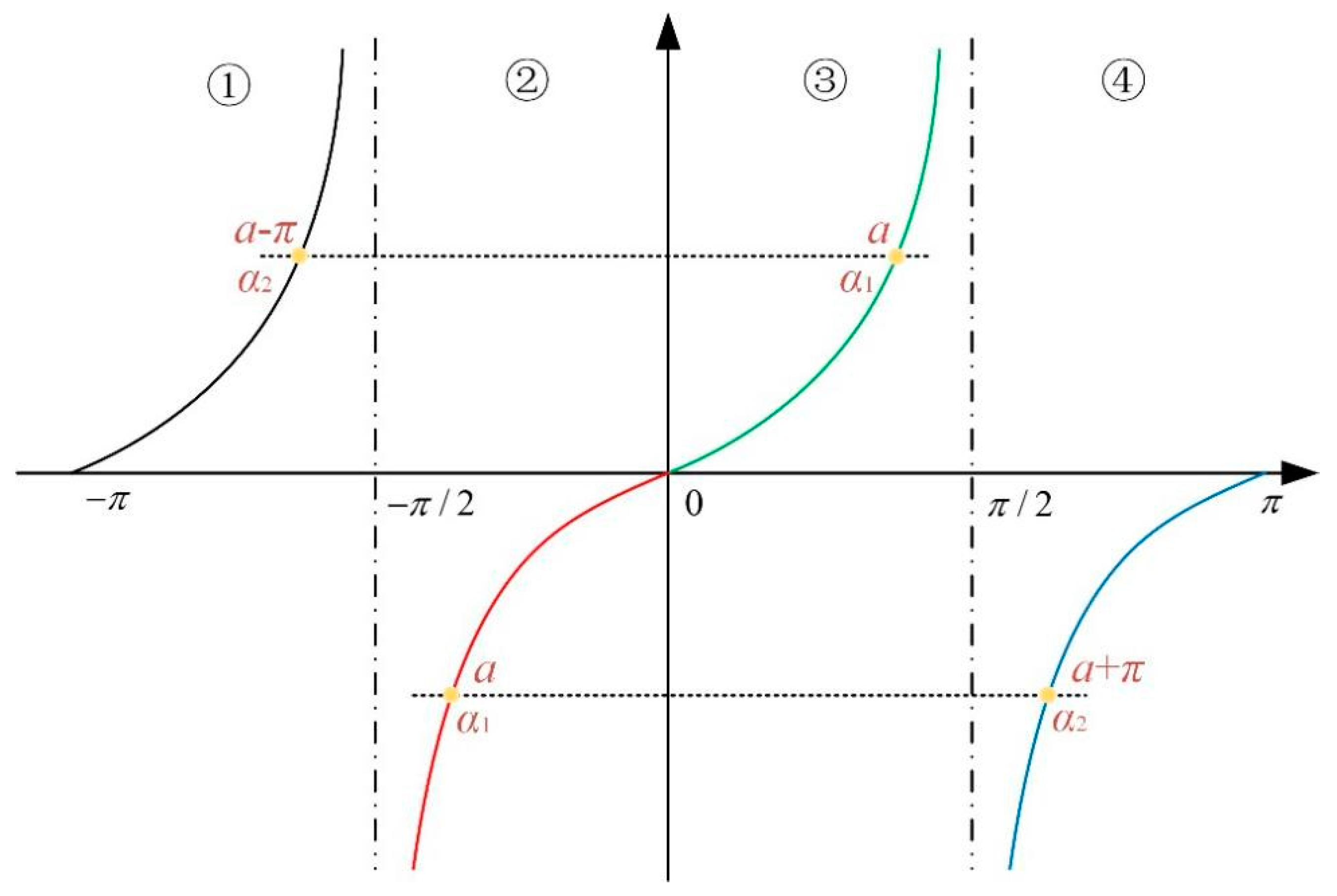
2.2. All Possible Solutions of Joint Angle in Inverse Kinematics

For the kinematic modeling of robots established by POE theory, the Paden–Kahan subproblem is needed to solve the inverse kinematics. It requires the tool coordinate system relative to the base coordinate system. As shown in Figure 2, [P_x,P_y,P_z]^T was converted to the base coordinate system and expressed as [P_x’,P_y’,P_z’]^T in the base coordinate system, where P_x’ = P_x + U_x, P_y’ = P_y + U_y, P_z’ = P_z + U_z.

Firstly, ignoring the periodicity of trigonometric functions and the stroke range of the rotation axis, one rotation angle a, b, and c of the A-joint, B-joint, and C-joint was calculated as

$$\{\begin{array}{l}\mathrm{a}=\arctan \frac{{\mathrm{P}}_{\mathrm{y}}^{\prime }}{{\mathrm{P}}_{\mathrm{x}}^{\prime }}\\ \mathrm{b}=\arctan \frac{{\mathrm{P}}_{\mathrm{z}}^{\prime }-{\mathrm{d}}_1+{\mathrm{a}}_5}{\mathrm{r}\pm {\mathrm{a}}_1-{\mathrm{a}}_4}\pm \arccos \frac{{\mathrm{a}}_2{}^2+{\left(\mathrm{r}\pm {\mathrm{a}}_1-{\mathrm{a}}_4\right)}^2+{\left({\mathrm{P}}_{\mathrm{z}}^{\prime }-{\mathrm{d}}_1+{\mathrm{a}}_5\right)}^2-{\mathrm{a}}_3{}^2}{2{\mathrm{a}}_2\sqrt{{\left(\mathrm{r}\pm {\mathrm{a}}_1-{\mathrm{a}}_4\right)}^2+{\left({\mathrm{P}}_{\mathrm{z}}^{\prime }-{\mathrm{d}}_1+{\mathrm{a}}_5\right)}^2}}\\ \mathrm{c}=\pm \arccos \frac{{\mathrm{a}}_2{}^2+{\mathrm{a}}_3{}^2-{\left(\mathrm{r}\pm {\mathrm{a}}_1-{\mathrm{a}}_4\right)}^2-{\left({\mathrm{P}}_{\mathrm{z}}^{\prime }-{\mathrm{d}}_1+{\mathrm{a}}_5\right)}^2}{2{\mathrm{a}}_2{\mathrm{a}}_3}\end{array},$$

(10)

where $\mathrm{r}=\sqrt{{\mathrm{P}}_{\mathrm{x}}^{\prime }{}^2+{\mathrm{P}}_{\mathrm{y}}^{\prime }{}^2}$.

Secondly, considering the periodicity of trigonometric function and the travel range of rotation axis, according to the structure of the multijoint industrial robot, the stroke range of α was [−π, π], the stroke range of β was [−π/2, 3π/2], and the stroke range of γ was [−π, π]. The range of the inverse trigonometric function and the stroke range of the A-joint, B-joint, and C-joint are shown in

Table 1. The range of inverse trigonometric functions and the stroke of rotation axes.

Solution of Rotation Angles	Range of Inverse Trigonometric Functions	Stroke of A-Joint, B-Joint, or C-Joint
$\mathrm{a}=\arctan ({\mathrm{P}}_{\mathrm{y}}^{\prime }/{\mathrm{P}}_{\mathrm{x}}^{\prime })$	$\left[-\mathrm{\pi }/2,\mathrm{\pi }/2\right]$	$\left[-\mathrm{\pi },\mathrm{\pi }\right]$
$\mathrm{b}=\arctan \frac{{\mathrm{P}}_{\mathrm{z}}^{\prime }-{\mathrm{d}}_1+{\mathrm{a}}_5}{\mathrm{r}\pm {\mathrm{a}}_1-{\mathrm{a}}_4}\pm \arccos \frac{{\mathrm{a}}_2{}^2+{\left(\mathrm{r}\pm {\mathrm{a}}_1-{\mathrm{a}}_4\right)}^2+{\left({\mathrm{P}}_{\mathrm{z}}^{\prime }-{\mathrm{d}}_1+{\mathrm{a}}_5\right)}^2-{\mathrm{a}}_3{}^2}{2{\mathrm{a}}_2\sqrt{{\left(\mathrm{r}\pm {\mathrm{a}}_1-{\mathrm{a}}_4\right)}^2+{\left({\mathrm{P}}_{\mathrm{z}}^{\prime }-{\mathrm{d}}_1+{\mathrm{a}}_5\right)}^2}}$	$\left[-3\mathrm{\pi }/2,3\mathrm{\pi }/2\right]$	$\left[-\mathrm{\pi }/2,3\mathrm{\pi }/2\right]$
$\mathrm{c}=\pm \arccos \frac{{\mathrm{a}}_2{}^2+{\mathrm{a}}_3{}^2-{\left(\mathrm{r}\pm {\mathrm{a}}_1-{\mathrm{a}}_4\right)}^2-{\left({\mathrm{P}}_{\mathrm{z}}^{\prime }-{\mathrm{d}}_1+{\mathrm{a}}_5\right)}^2}{2{\mathrm{a}}_2{\mathrm{a}}_3}$	$\left[-\mathrm{\pi },\mathrm{\pi }\right]$	$\left[-\mathrm{\pi },\mathrm{\pi }\right]$

. For the A-joint, when the range of α was [−π, π], the tangent function was as shown in Figure 3. Thus, the stroke range of equations were divided into four regions, and the dual solution of equations is shown in

Table 2. The solutions of the joint angle of the A-joint.

$\mathrm{a}=\arctan ({\mathrm{P}}_{\mathrm{y}}^{\prime }/{\mathrm{P}}_{\mathrm{x}}^{\prime })$	Double Solutions of α	Region Belonged to
a > 0	${\mathrm{\alpha }}_1=\mathrm{a}$ ${\mathrm{\alpha }}_2=\mathrm{a}-\mathrm{\pi }$	③ ①
a < 0	${\mathrm{\alpha }}_1=\mathrm{a}$ ${\mathrm{\alpha }}_2=\mathrm{a}+\mathrm{\pi }$	② ④
a = 0	${\mathrm{\alpha }}_1=0$ ${\mathrm{\alpha }}_2=\mathrm{\pi }$	- -

.

Combining the solutions of joint angles of the A-joint, B-joint, and C-joint, the four solutions of (α, β, γ) were represented as follows. When P_x = 0, $\mathrm{r}=\sqrt{{\left({\mathrm{P}}_{\mathrm{x}}+{\mathrm{U}}_{\mathrm{x}}\right)}^2+{\left({\mathrm{P}}_{\mathrm{y}}+{\mathrm{U}}_{\mathrm{y}}\right)}^2}$, the solutions were represented as

$$\{\begin{array}{l}\mathrm{a}=\pm \frac{\mathrm{\pi }}{2}\\ \mathrm{b}=\arctan \frac{{\mathrm{P}}_{\mathrm{z}}+{\mathrm{U}}_{\mathrm{z}}-{\mathrm{d}}_1+{\mathrm{a}}_5}{\mathrm{r}\pm {\mathrm{a}}_1-{\mathrm{a}}_4}\pm \arccos \frac{{\mathrm{a}}_2{}^2+{\left(\mathrm{r}\pm {\mathrm{a}}_1-{\mathrm{a}}_4\right)}^2+{\left({\mathrm{P}}_{\mathrm{z}}+{\mathrm{U}}_{\mathrm{z}}-{\mathrm{d}}_1+{\mathrm{a}}_5\right)}^2-{\mathrm{a}}_3{}^2}{2{\mathrm{a}}_2\sqrt{{\left(\mathrm{r}\pm {\mathrm{a}}_1-{\mathrm{a}}_4\right)}^2+{\left({\mathrm{P}}_{\mathrm{z}}+{\mathrm{U}}_{\mathrm{z}}-{\mathrm{d}}_1+{\mathrm{a}}_5\right)}^2}}\\ \mathrm{c}=\pm \arccos \frac{{\mathrm{a}}_2{}^2+{\mathrm{a}}_3{}^2-{\left(\mathrm{r}\pm {\mathrm{a}}_1-{\mathrm{a}}_4\right)}^2-{\left({\mathrm{P}}_{\mathrm{z}}+{\mathrm{U}}_{\mathrm{z}}-{\mathrm{d}}_1+{\mathrm{a}}_5\right)}^2}{2{\mathrm{a}}_2{\mathrm{a}}_3}\end{array}$$

(11)

when Px ≠ 0, $\mathrm{a}=\arctan \left[\left({\mathrm{P}}_{\mathrm{y}}+{\mathrm{U}}_{\mathrm{y}}\right)/\left({\mathrm{P}}_{\mathrm{x}}+{\mathrm{U}}_{\mathrm{x}}\right)\right]$, $\mathrm{r}=\sqrt{{\left({\mathrm{P}}_{\mathrm{x}}+{\mathrm{U}}_{\mathrm{x}}\right)}^2+{\left({\mathrm{P}}_{\mathrm{y}}+{\mathrm{U}}_{\mathrm{y}}\right)}^2}$. When α, β, and γ are all within the feasible domain, there were four groups of solutions. As an example, when a > 0, the four groups of solutions were as follows.

$$\{\begin{array}{l}{\mathrm{\alpha }}_1=\mathrm{a}\\ {\mathsf{\beta }}_1=\arctan \frac{{\mathrm{P}}_{\mathrm{z}}+{\mathrm{U}}_{\mathrm{z}}-{\mathrm{d}}_1+{\mathrm{a}}_5}{\mathrm{r}-{\mathrm{a}}_1-{\mathrm{a}}_4}+\arccos \frac{{\mathrm{a}}_2{}^2+{\left(\mathrm{r}-{\mathrm{a}}_1-{\mathrm{a}}_4\right)}^2+{\left({\mathrm{P}}_{\mathrm{z}}+{\mathrm{U}}_{\mathrm{z}}-{\mathrm{d}}_1+{\mathrm{a}}_5\right)}^2-{\mathrm{a}}_3{}^2}{2{\mathrm{a}}_2\sqrt{{\left(\mathrm{r}-{\mathrm{a}}_1-{\mathrm{a}}_4\right)}^2+{\left({\mathrm{P}}_{\mathrm{z}}+{\mathrm{U}}_{\mathrm{z}}-{\mathrm{d}}_1+{\mathrm{a}}_5\right)}^2}}\\ {\mathsf{\gamma }}_1=\arccos \frac{{\mathrm{a}}_2{}^2+{\mathrm{a}}_3{}^2-{\left(\mathrm{r}-{\mathrm{a}}_1-{\mathrm{a}}_4\right)}^2-{\left({\mathrm{P}}_{\mathrm{z}}+{\mathrm{U}}_{\mathrm{z}}-{\mathrm{d}}_1+{\mathrm{a}}_5\right)}^2}{2{\mathrm{a}}_2{\mathrm{a}}_3}\end{array}$$

(12)

$$\{\begin{array}{l}{\mathrm{\alpha }}_1=\mathrm{a}\\ {\mathsf{\beta }}_2=\arctan \frac{{\mathrm{P}}_{\mathrm{z}}+{\mathrm{U}}_{\mathrm{z}}-{\mathrm{d}}_1+{\mathrm{a}}_5}{\mathrm{r}-{\mathrm{a}}_1-{\mathrm{a}}_4}-\arccos \frac{{\mathrm{a}}_2{}^2+{\left(\mathrm{r}-{\mathrm{a}}_1-{\mathrm{a}}_4\right)}^2+{\left({\mathrm{P}}_{\mathrm{z}}+{\mathrm{U}}_{\mathrm{z}}-{\mathrm{d}}_1+{\mathrm{a}}_5\right)}^2-{\mathrm{a}}_3{}^2}{2{\mathrm{a}}_2\sqrt{{\left(\mathrm{r}-{\mathrm{a}}_1-{\mathrm{a}}_4\right)}^2+{\left({\mathrm{P}}_{\mathrm{z}}+{\mathrm{U}}_{\mathrm{z}}-{\mathrm{d}}_1+{\mathrm{a}}_5\right)}^2}}\\ {\mathsf{\gamma }}_2=-\arccos \frac{{\mathrm{a}}_2{}^2+{\mathrm{a}}_3{}^2-{\left(\mathrm{r}-{\mathrm{a}}_1-{\mathrm{a}}_4\right)}^2-{\left({\mathrm{P}}_{\mathrm{z}}+{\mathrm{U}}_{\mathrm{z}}-{\mathrm{d}}_1+{\mathrm{a}}_5\right)}^2}{2{\mathrm{a}}_2{\mathrm{a}}_3}\end{array}$$

(13)

$$\{\begin{array}{l}{\mathrm{\alpha }}_2=\mathrm{a}-\mathrm{\pi }\\ {\mathsf{\beta }}_1=\arctan \frac{{\mathrm{P}}_{\mathrm{z}}+{\mathrm{U}}_{\mathrm{z}}-{\mathrm{d}}_1+{\mathrm{a}}_5}{\mathrm{r}-{\mathrm{a}}_1-{\mathrm{a}}_4}+\arccos \frac{{\mathrm{a}}_2{}^2+{\left(\mathrm{r}+{\mathrm{a}}_1-{\mathrm{a}}_4\right)}^2+{\left({\mathrm{P}}_{\mathrm{z}}+{\mathrm{U}}_{\mathrm{z}}-{\mathrm{d}}_1+{\mathrm{a}}_5\right)}^2-{\mathrm{a}}_3{}^2}{2{\mathrm{a}}_2\sqrt{{\left(\mathrm{r}-{\mathrm{a}}_1-{\mathrm{a}}_4\right)}^2+{\left({\mathrm{P}}_{\mathrm{z}}+{\mathrm{U}}_{\mathrm{z}}-{\mathrm{d}}_1+{\mathrm{a}}_5\right)}^2}}\\ {\mathsf{\gamma }}_1=\arccos \frac{{\mathrm{a}}_2{}^2+{\mathrm{a}}_3{}^2-{\left(\mathrm{r}+{\mathrm{a}}_1-{\mathrm{a}}_4\right)}^2-{\left({\mathrm{P}}_{\mathrm{z}}+{\mathrm{U}}_{\mathrm{z}}-{\mathrm{d}}_1+{\mathrm{a}}_5\right)}^2}{2{\mathrm{a}}_2{\mathrm{a}}_3}\end{array}$$

(14)

$$\{\begin{array}{l}{\mathrm{\alpha }}_2=\mathrm{a}-\mathrm{\pi }\\ {\mathsf{\beta }}_2=\arctan \frac{{\mathrm{P}}_{\mathrm{z}}+{\mathrm{U}}_{\mathrm{z}}-{\mathrm{d}}_1+{\mathrm{a}}_5}{\mathrm{r}+{\mathrm{a}}_1-{\mathrm{a}}_4}-\arccos \frac{{\mathrm{a}}_2{}^2+{\left(\mathrm{r}+{\mathrm{a}}_1-{\mathrm{a}}_4\right)}^2+{\left({\mathrm{P}}_{\mathrm{z}}+{\mathrm{U}}_{\mathrm{z}}-{\mathrm{d}}_1+{\mathrm{a}}_5\right)}^2-{\mathrm{a}}_3{}^2}{2{\mathrm{a}}_2\sqrt{{\left(\mathrm{r}+{\mathrm{a}}_1-{\mathrm{a}}_4\right)}^2+{\left({\mathrm{P}}_{\mathrm{z}}+{\mathrm{U}}_{\mathrm{z}}-{\mathrm{d}}_1+{\mathrm{a}}_5\right)}^2}}\\ {\mathsf{\gamma }}_2=-\arccos \frac{{\mathrm{a}}_2{}^2+{\mathrm{a}}_3{}^2-{\left(\mathrm{r}+{\mathrm{a}}_1-{\mathrm{a}}_4\right)}^2-{\left({\mathrm{P}}_{\mathrm{z}}+{\mathrm{U}}_{\mathrm{z}}-{\mathrm{d}}_1+{\mathrm{a}}_5\right)}^2}{2{\mathrm{a}}_2{\mathrm{a}}_3}\end{array}$$

(15)

For the multijoint robot shown in Figure 1, the A-joint is the first joint, B-joint is the second joint, and C-joint is the third joint. All possible groups of joint angles of one pose for this robot can be represented as follows.

$$\{\begin{array}{l}{{}_1\mathrm{Q}}_{\mathrm{i}}={[{{}_1\mathsf{\theta }}_{1,\mathrm{i}},{{}_1\mathsf{\theta }}_{2,\mathrm{i}},{{}_1\mathsf{\theta }}_{3,\mathrm{i}}]}^{\mathrm{T}}={[{\mathrm{\alpha }}_1,{\mathsf{\beta }}_1,{\mathsf{\gamma }}_1]}^{\mathrm{T}}\\ {{}_2\mathrm{Q}}_{\mathrm{i}}={[{{}_2\mathsf{\theta }}_{1,\mathrm{i}},{{}_2\mathsf{\theta }}_{2,\mathrm{i}},{{}_2\mathsf{\theta }}_{3,\mathrm{i}}]}^{\mathrm{T}}={[{\mathrm{\alpha }}_1,{\mathsf{\beta }}_2,{\mathsf{\gamma }}_2]}^{\mathrm{T}}\\ {{}_3\mathrm{Q}}_{\mathrm{i}}={[{{}_3\mathsf{\theta }}_{1,\mathrm{i}},{{}_3\mathsf{\theta }}_{2,\mathrm{i}},{{}_3\mathsf{\theta }}_{3,\mathrm{i}}]}^{\mathrm{T}}={[{\mathrm{\alpha }}_2,{\mathsf{\beta }}_1,{\mathsf{\gamma }}_1]}^{\mathrm{T}}\\ {{}_4\mathrm{Q}}_{\mathrm{i}}={[{{}_4\mathsf{\theta }}_{1,\mathrm{i}},{{}_4\mathsf{\theta }}_{2,\mathrm{i}},{{}_4\mathsf{\theta }}_{3,\mathrm{i}}]}^{\mathrm{T}}={[{\mathrm{\alpha }}_2,{\mathsf{\beta }}_2,{\mathsf{\gamma }}_2]}^{\mathrm{T}}\end{array}$$

where _qQ_i represents the qth possible group of solutions of the point P_i.; _qθ_h,i represents the joint angle of the hth joint in the qth possible group of solutions.

3. Multisolution Selection of Joint Angle Based on the Key Order of the Joint

Four groups of possible solutions can be obtained for one path point. The solutions should be compared and analyzed to obtain the appropriate solution for the actual control and the motion of the robot. This section proposes one multisolution selection method to obtain the appropriate group of joint angles from the four groups of possible solutions. The key order of the joints is determined by comparing the sensitivity of all joint angles. The possible solutions are selected by comparing the increment of joint angles one by one, according to the key degree of all joints.

3.1. Key Order of the Joint

When the multijoint industrial robot is running according to the specified path, the rotation or movement of different joints may have different effects on the end position, which may affect the positioning accuracy of the robot. The appropriate solutions can be selected based on the influences of the joints on the robot, which can evaluate the key degree of the joints.

Sensitivity is introduced to evaluate the influence of each joint on the end position. Generally, sensitivity refers to the ratio of independent variable change to dependent variable change in a system. For sensitivity analysis of the joint in this paper, the angles of each joint of the multijoint industrial robot were regarded as independent variables of the system, and the dependent variable was the displacement of the end of the robot in a single direction. The sensitivity component of the hth joint in one direction can be obtained by calculating the partial derivative of the angle of the hth joint with respect to the positon of the robot end-effector in this direction, that is,

$${\mathrm{S}}_{\mathrm{k}}=\frac{\partial {\mathrm{P}}_{\mathrm{k}}}{\partial {\mathsf{\theta }}_{\mathrm{h}}}\begin{array}{cc},& \mathrm{h}\in \left[1,\mathrm{m}\right],\mathrm{k}=\mathrm{x},\mathrm{y},\mathrm{z}\end{array}$$

where P_k is the position of the robot end-effector in the k direction; θ_h is the joint angle of the hth joint, and m is the number of joints of the robot.

Further, in order to understand the effect of rotation or movement of a single joint on the end position of the robot, the sensitivity of a joint to the end position can be expressed by S_θh, that is,

$${\mathrm{S}}_{{\mathsf{\theta }}_{\mathrm{h}}}=\sqrt{{\mathrm{S}}_{\mathrm{x}}^2+{\mathrm{S}}_{\mathrm{y}}^2+{\mathrm{S}}_{\mathrm{z}}^2}=\sqrt{{\left(\frac{\partial {\mathrm{P}}_{\mathrm{x}}}{\partial {\mathsf{\theta }}_{\mathrm{h}}}\right)}^2+{\left(\frac{\partial {\mathrm{P}}_{\mathrm{y}}}{\partial {\mathsf{\theta }}_{\mathrm{h}}}\right)}^2+{\left(\frac{\partial {\mathrm{P}}_{\mathrm{z}}}{\partial {\mathsf{\theta }}_{\mathrm{h}}}\right)}^2}$$

where P = (P_x, P_y, P_z) is the path point of the robot. The sensitivity of each joint can be solved by Jacobian matrix. The Jacobian matrix J can be obtained from Equation (15).

$$\mathrm{J}=\left[\begin{array}{c}\begin{array}{cccc}\frac{\partial {\mathrm{P}}_{\mathrm{x}}}{\partial {\mathsf{\theta }}_1}& \frac{\partial {\mathrm{P}}_{\mathrm{x}}}{\partial {\mathsf{\theta }}_2}& \cdots & \frac{\partial {\mathrm{P}}_{\mathrm{x}}}{\partial {\mathsf{\theta }}_{\mathrm{m}}}\end{array}\\ \begin{array}{cccc}\frac{\partial {\mathrm{P}}_{\mathrm{y}}}{\partial {\mathsf{\theta }}_1}& \frac{\partial {\mathrm{P}}_{\mathrm{y}}}{\partial {\mathsf{\theta }}_2}& \cdots & \frac{\partial {\mathrm{P}}_{\mathrm{y}}}{\partial {\mathsf{\theta }}_{\mathrm{m}}}\end{array}\\ \begin{array}{cccc}\frac{\partial {\mathrm{P}}_{\mathrm{z}}}{\partial {\mathsf{\theta }}_1}& \frac{\partial {\mathrm{P}}_{\mathrm{z}}}{\partial {\mathsf{\theta }}_2}& \cdots & \frac{\partial {\mathrm{P}}_{\mathrm{z}}}{\partial {\mathsf{\theta }}_{\mathrm{m}}}\end{array}\end{array}\right]$$

The sensitivity can be used to evaluate the degrees of influence of the joints on the precision of the robot, so the sensitivity can be used to present the key degree of a joint. According to the sensitivity of all joints, joints are sorted from high key degree to low key degree. The sequence of each joint after sorting is the key order of the joint, which is from one to the number of the joints in the robot. For example, if the sequence of the hth joint after sorting is j, then the key order of the hth joint d_h is j, and the hth joint also is jth key joint.

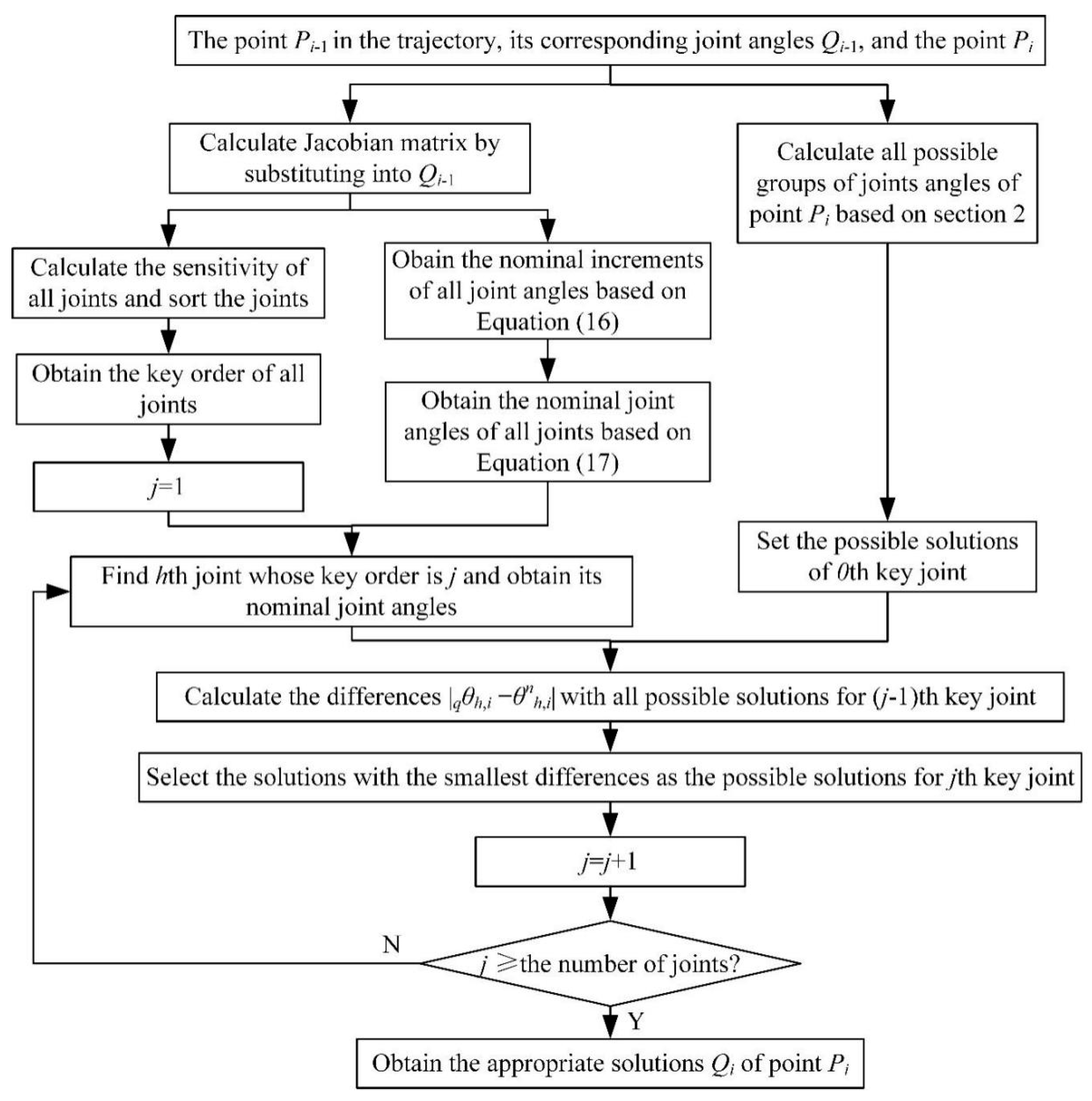
3.2. Multisolution Selection

Even though each solution is available for the kinematics in theory, it is necessary to select one appropriate solution of joint angles from the view of a whole tool path and precise machining. The magnitude of joint motion is directly related to the energy consumption and running time of the entire robot system, and it is also important to ensure that continuous changes in joint angles do not mutate. The incremental changes of each joint angle should be small enough that the relative motion amplitude of the joint between the two path points can be considered in path planning. The key joints and joint increments are used to select a suitable solution from all possible solutions in the inverse kinematics of a multijoint industrial robot.

For one point P_i = [x_i, y_i, z_i]^T in the trajectory of the end-effector of the robot, all possible groups of joint angles can be obtained based on Section 2. The previous point P_i−1 in the trajectory and its corresponding joint angles of the robot Q_i−1 = [θ_{1, i−1}, θ_{2, i−1}, ∙∙∙, θ_{m, i−1}]T are used to select the appropriate solutions Q_i of the point P_i. The nominal increments of all joint angles from P_i-1 to P_i can be calculated with the Jacobian matrix by substituting in the joint angles Q_i−1 of P_i−1 as

$$\mathrm{\Delta }{\mathrm{Q}}_{\mathrm{i}}={[\mathrm{\Delta }{\mathsf{\theta }}_{1,\mathrm{i}},\mathrm{\Delta }{\mathsf{\theta }}_{2,\mathrm{i}},\dots ,\mathrm{\Delta }{\mathsf{\theta }}_{\mathrm{m},\mathrm{i}}]}^{\mathrm{T}}={\left({\mathrm{J}}_{\mathrm{i}-1}^{\mathrm{T}}\cdot {\mathrm{J}}_{\mathrm{i}-1}\right)}^{-1}\cdot {\mathrm{J}}_{\mathrm{i}-1}^{\mathrm{T}}\cdot ({\mathrm{P}}_{\mathrm{i}}-{\mathrm{P}}_{\mathrm{i}-1})$$

(16)

The nominal joint angles of point P_i can be obtained with the joint angles Q_i-1 as

$${\mathrm{Q}}_{\mathrm{i}}^{\mathrm{n}}={\mathrm{Q}}_{\mathrm{i}-1}+\mathrm{\Delta }{\mathrm{Q}}_{\mathrm{i}}={[{\mathsf{\theta }}_{1,\mathrm{i}}^{\mathrm{n}},{\mathsf{\theta }}_{2,\mathrm{i}}^{\mathrm{n}},\dots ,{\mathsf{\theta }}_{\mathrm{m},\mathrm{i}}^{\mathrm{n}}]}^{\mathrm{T}}$$

(17)

where ΔQ_i represents the nominal increments of all joint angles of P_i; Δθ_k,i represents the nominal increments of the kth joint; J_i−1 represents the Jacobian matrix by substituting into joint angles Q_i−1; ${\mathrm{Q}}_{\mathrm{i}}^{\mathrm{n}}$ represents the nominal joint angles of point P_i; and ${\mathsf{\theta }}_{\mathrm{k},\mathrm{i}}^{\mathrm{n}}$ represents the nominal joint angles of kth joint.

All joints are sorted based on their key degree, and the key order of all joints can be obtained. For example, if the key order of the hth joint d_h = j, it means that the hth joint is the jth key joint. The nominal joint angles of the jth key joint for point P_i can then be obtained as

$${\mathsf{\theta }}_{\mathrm{j},\mathrm{i}}^{\mathrm{d}}={\mathsf{\theta }}_{\mathrm{h},\mathrm{i}}^{\mathrm{n}}$$

(18)

where ${\mathsf{\theta }}_{\mathrm{j},\mathrm{i}}^{\mathrm{d}}$ represents the nominal joint angles of the jth key joint.

One principle based on the smallest differences of the nominal angle for one joint is proposed to select the possible solutions for this joint. The possible joint angles of one joint _qθ_h,i in the possible groups of solutions obtained by the inverse kinematics can be compared with the nominal joint angles ${\mathsf{\theta }}_{\mathrm{h},\mathrm{i}}^{\mathrm{n}}$ of this joint obtained by Equations (16) and (17). The differences can be expressed as $\left|{}_{\mathrm{q}}{\mathsf{\theta }}_{\mathrm{h},\mathrm{i}}-{\mathsf{\theta }}_{\mathrm{h},\mathrm{i}}^{\mathrm{n}}\right|$. The selection principle for one joint is to obtain the smallest differences of joint angles. In this way, the possible solutions for one joint are selected from all possible groups of solutions. The key order of one joint reflects the key degree of the influences of this joint. The possible solutions for the joints with low key order should be selected before selecting the solutions for the joints with high key order. Namely, the possible solutions for the jth key joint can be selected from the possible solutions for the (j−1)th key joint, and all possible groups of solutions obtained in Section 2 can be seen as the possible solutions for the 0th key joint.

The flow chart of the multisolution selection method based on the key order of joints for the appropriate solution of joint angles at one point in the trajectory of the robot is presented in Figure 4. First, all possible groups of joint angles of point P_i are obtained based on Section 2 to serve as the possible solutions of the 0th key joint. Secondly, the Jacobian matrix is obtained by substituting in joint angles of point P_i-1. The sensitivities of all joints are calculated with the Jacobian matrix to sort the joints and obtain the key order of all joints. The nominal increments and the nominal joint angles of all joints are calculated based on Equations (16) and (17), with the Jacobian matrix. Thirdly, the possible solutions of all joints are selected according to the key order of all joints, applying the principle based on smallest differences of the nominal angles. When key order is j, the joint with the key order j is found by comparing the key orders of all joints with j in order to obtain its nominal joint angles. The differences between this nominal joint angle and the corresponding joint angles of all possible solutions for the (j−1)th key joint are calculated. The possible solutions for the jth key joint are the solutions with the smallest differences of the joint angles of this joint. When j is larger than the number of joints of the robot, the possible solutions for all joints are obtained. The possible solutions for the joint with largest key order are the appropriate solutions for point P_i of the robot.

4. A Workspace Visualization Method Based on a 3D-Printing Layering Concept

4.1. Existing Boundary Extraction Method

A numerical Monte-Carlo-based method is adopted to obtain the shape and size of the workspace [32], as shown in the point cloud in Figure 5. This is a simple method to describe a workspace boundary from an engineering perspective. The principle of workspace generation is the mapping relationship between joint variables and workspace. The three joint variables are assigned the same number of random values in their respective motion ranges, and then mapped to the workspace through kinematics equations; thus, a three-dimensional workspace point cloud is formed.

Assuming that the point cloud in the XY plane is extracted when Z = 200 mm, as shown in Figure 6, it may be found that the workspace shape described by the point cloud is not accurate enough. Figure 7 shows the boundary curve formed by extracting the boundary contour of the workspace in Figure 6. The boundary curve presents an irregular curve, which is quite different from the actual regular curve. This deviation has a negative impact not only on the shape, but also on the area and volume estimation of the workspace. This section presents a new method to obtain more accurate boundary.

4.2. Extraction of the Workspace Boundary Based on 3D-Layering Concept

In order to simplify the problem, the concept of 3D-printing layering was used to divide the workspace into many slices along the Z direction, so that the three-dimensional space problem can be converted to a two-dimensional plane. The set of point P is defined as the workspace of the robot, and the generalized joint variables are written as parametric equations, namely

$$\mathrm{W}=\{\begin{array}{c}{\mathrm{P}}_{\mathrm{x}}\left({\mathsf{\theta }}_{\mathrm{i}}\right)\\ {\mathrm{P}}_{\mathrm{y}}\left({\mathsf{\theta }}_{\mathrm{i}}\right)\\ {\mathrm{P}}_{\mathrm{z}}\left({\mathsf{\theta }}_{\mathrm{i}}\right)\end{array}\begin{array}{cc}& \end{array}{\mathsf{\theta }}_{\mathrm{i}\min }\le {\mathsf{\theta }}_{\mathrm{i}}\le {\mathsf{\theta }}_{\mathrm{i}\max }$$

(19)

where θ_i = (α_i, β_i, γ_i). From the kinematics Equation (5), the contour boundary equation can be derived as

$${\left({\mathrm{P}}_{\mathrm{x}}+{\mathrm{U}}_{\mathrm{x}}\right)}^2+{\left({\mathrm{P}}_{\mathrm{y}}+{\mathrm{U}}_{\mathrm{y}}\right)}^2={\left[{\mathrm{a}}_3\cos \left(\mathsf{\beta }+\mathsf{\gamma }\right)+{\mathrm{a}}_2\cos \mathsf{\beta }+{\mathrm{a}}_1+{\mathrm{a}}_4\right]}^2$$

(20)

From the boundary equation, it can be seen that the boundary of the contour should be a circle or annulus in the XY plane, of which the center is

$$\{\begin{array}{l}{\mathrm{r}}_{\mathrm{x}}=-{\mathrm{U}}_{\mathrm{x}}\\ {\mathrm{r}}_{\mathrm{y}}=-{\mathrm{U}}_{\mathrm{y}}\end{array}$$

(21)

and the radius is

$$\mathrm{r}={\mathrm{a}}_3\cos \left(\mathsf{\beta }+\mathsf{\gamma }\right)+{\mathrm{a}}_2\cos \mathsf{\beta }+{\mathrm{a}}_1+{\mathrm{a}}_4$$

(22)

In order to solve the minimum and maximum problems of r, γ is expressed as β by the kinematics Equation (8), namely

$$\cos \left(\mathsf{\beta }+\mathsf{\gamma }\right)=\pm \sqrt{1-{\left(\frac{{\mathrm{P}}_{\mathrm{z}}-{\mathrm{a}}_2\sin \mathsf{\beta }-{\mathrm{d}}_1+{\mathrm{a}}_5+{\mathrm{U}}_{\mathrm{z}}}{{\mathrm{a}}_3}\right)}^2}$$

(23)

The above expression is substituted into Equation (22), giving

$$\mathrm{r}=\pm \sqrt{{\mathrm{a}}_3^2-{\left({\mathrm{P}}_{\mathrm{z}}-{\mathrm{a}}_2\sin \mathsf{\beta }-{\mathrm{d}}_1+{\mathrm{a}}_5+{\mathrm{U}}_{\mathrm{z}}\right)}^2}+{\mathrm{a}}_2\cos \mathsf{\beta }+{\mathrm{a}}_1+{\mathrm{a}}_4$$

(24)

As can be seen from the expression of radius r, the radius is only related to the variable β at a given height. According to the kinematics Formula (5) of the multijoint industrial robot, the relationship between β and γ can be obtained as

$$\mathsf{\beta }=\arcsin \frac{{\mathrm{a}}_3\left({\mathrm{P}}_{\mathrm{z}}-{\mathrm{d}}_1+{\mathrm{a}}_5+{\mathrm{U}}_{\mathrm{z}}\right)}{\sqrt{{\mathrm{a}}_2^2+2{\mathrm{a}}_2{\mathrm{a}}_3\cos \mathsf{\gamma }+{\mathrm{a}}_3^2}}-\arctan \frac{{\mathrm{a}}_3\sin \mathsf{\gamma }}{{\mathrm{a}}_2+{\mathrm{a}}_3\cos \mathsf{\gamma }}$$

(25)

Figure 8 is a contour of the workspace in the XZ plane. The contour is divided into four parts: FG, GM, ME, and EF. The maximum radius of the boundary of each layer of the workspace in the XY plane is on the contour segment EF, and the minimum radius is on the contour segments FG, GM, and ME. According to the structural parameters and the joint-angle stroke range of the multijoint industrial robot, the condition for forming the contour segment EF (i.e., the outer contour of the workspace) is that when the joint angle γ of the robot takes the maximum, that is, γ = γ_max.

$$\mathsf{\beta }=\arcsin \frac{{\mathrm{a}}_3\left({\mathrm{P}}_{\mathrm{z}}-{\mathrm{d}}_1+{\mathrm{a}}_5+{\mathrm{U}}_{\mathrm{z}}\right)}{\sqrt{{\mathrm{a}}_2^2+2{\mathrm{a}}_2{\mathrm{a}}_3\cos {\mathsf{\gamma }}_{\max }+{\mathrm{a}}_3^2}}-\arctan \frac{{\mathrm{a}}_3\sin {\mathsf{\gamma }}_{\max }}{{\mathrm{a}}_2+{\mathrm{a}}_3\cos {\mathsf{\gamma }}_{\max }}$$

(26)

Similarly, the condition for forming the contour segment GM is that when the joint angle γ of the robot takes the minimum, that is, γ = γ_min.

$$\mathsf{\beta }=\arcsin \frac{{\mathrm{a}}_3\left({\mathrm{P}}_{\mathrm{z}}-{\mathrm{d}}_1+{\mathrm{a}}_5+{\mathrm{U}}_{\mathrm{z}}\right)}{\sqrt{{\mathrm{a}}_2^2+2{\mathrm{a}}_2{\mathrm{a}}_3\cos {\mathsf{\gamma }}_{\min }+{\mathrm{a}}_3^2}}-\arctan \frac{{\mathrm{a}}_3\sin {\mathsf{\gamma }}_{\min }}{{\mathrm{a}}_2+{\mathrm{a}}_3\cos {\mathsf{\gamma }}_{\min }}$$

(27)

The condition for forming the contour segment FG is that when the joint angle β of the robot takes the maximum, that is, β = β_max. Similarly, the condition for forming the contour segment ME is that when the joint angle γ of the robot takes the minimum, that is, β = β_min. Thus, the minimum and maximum of r in the XY plane can be obtained at a given height Z, as shown in

Table 3. The value of β when r takes the minimum and maximum at a given height Z.

The Scope of the Pz	The Value of β when rmin	The Value of β when rmax
$\begin{array}{c}{\mathrm{P}}_{\mathrm{z}}<{\mathrm{P}}_{\mathrm{z}}\left(0,{\mathsf{\gamma }}_{\min }\right)\\ ({\mathrm{L}}_1~{\mathrm{L}}_2)\end{array}$	${\mathsf{\beta }}_{\min }$	$\arcsin \frac{{\mathrm{a}}_3\left({\mathrm{P}}_{\mathrm{z}}-{\mathrm{d}}_1+{\mathrm{a}}_5+{\mathrm{U}}_{\mathrm{z}}\right)}{\sqrt{{\mathrm{a}}_2^2+2{\mathrm{a}}_2{\mathrm{a}}_3\cos {\mathsf{\gamma }}_{\max }+{\mathrm{a}}_3^2}}-\arctan \frac{{\mathrm{a}}_3\sin {\mathsf{\gamma }}_{\max }}{{\mathrm{a}}_2+{\mathrm{a}}_3\cos {\mathsf{\gamma }}_{\max }}$
$\begin{array}{c}{\mathrm{P}}_{\mathrm{z}}\left(0,{\mathsf{\gamma }}_{\min }\right)\le {\mathrm{P}}_{\mathrm{z}}<{\mathrm{P}}_{\mathrm{z}}\left({\mathsf{\beta }}_{\min },{\mathsf{\gamma }}_{\min }\right)\\ ({\mathrm{L}}_2~{\mathrm{L}}_3)\end{array}$	${\mathsf{\beta }}_{\min }$ $\arcsin \frac{{\mathrm{a}}_3\left({\mathrm{P}}_{\mathrm{z}}-{\mathrm{d}}_1+{\mathrm{a}}_5+{\mathrm{U}}_{\mathrm{z}}\right)}{\sqrt{{\mathrm{a}}_2^2+2{\mathrm{a}}_2{\mathrm{a}}_3\cos {\mathsf{\gamma }}_{\min }+{\mathrm{a}}_3^2}}-\arctan \frac{{\mathrm{a}}_3\sin {\mathsf{\gamma }}_{\min }}{{\mathrm{a}}_2+{\mathrm{a}}_3\cos {\mathsf{\gamma }}_{\min }}$	$\arcsin \frac{{\mathrm{a}}_3\left({\mathrm{P}}_{\mathrm{z}}-{\mathrm{d}}_1+{\mathrm{a}}_5+{\mathrm{U}}_{\mathrm{z}}\right)}{\sqrt{{\mathrm{a}}_2^2+2{\mathrm{a}}_2{\mathrm{a}}_3\cos {\mathsf{\gamma }}_{\min }+{\mathrm{a}}_3^2}}-\arctan \frac{{\mathrm{a}}_3\sin {\mathsf{\gamma }}_{\min }}{{\mathrm{a}}_2+{\mathrm{a}}_3\cos {\mathsf{\gamma }}_{\min }}$ $\arcsin \frac{{\mathrm{a}}_3\left({\mathrm{P}}_{\mathrm{z}}-{\mathrm{d}}_1+{\mathrm{a}}_5+{\mathrm{U}}_{\mathrm{z}}\right)}{\sqrt{{\mathrm{a}}_2^2+2{\mathrm{a}}_2{\mathrm{a}}_3\cos {\mathsf{\gamma }}_{\max }+{\mathrm{a}}_3^2}}-\arctan \frac{{\mathrm{a}}_3\sin {\mathsf{\gamma }}_{\max }}{{\mathrm{a}}_2+{\mathrm{a}}_3\cos {\mathsf{\gamma }}_{\max }}$
$\begin{array}{c}{\mathrm{P}}_{\mathrm{z}}\left({\mathsf{\beta }}_{\min },{\mathsf{\gamma }}_{\min }\right)\le {\mathrm{P}}_{\mathrm{z}}<{\mathrm{P}}_{\mathrm{z}}\left({\mathsf{\beta }}_{\max },{\mathsf{\gamma }}_{\min }\right)\\ ({\mathrm{L}}_3~{\mathrm{L}}_4)\end{array}$	$\arcsin \frac{{\mathrm{a}}_3\left({\mathrm{P}}_{\mathrm{z}}-{\mathrm{d}}_1+{\mathrm{a}}_5+{\mathrm{U}}_{\mathrm{z}}\right)}{\sqrt{{\mathrm{a}}_2^2+2{\mathrm{a}}_2{\mathrm{a}}_3\cos {\mathsf{\gamma }}_{\min }+{\mathrm{a}}_3^2}}-\arctan \frac{{\mathrm{a}}_3\sin {\mathsf{\gamma }}_{\min }}{{\mathrm{a}}_2+{\mathrm{a}}_3\cos {\mathsf{\gamma }}_{\min }}$	$\arcsin \frac{{\mathrm{a}}_3\left({\mathrm{P}}_{\mathrm{z}}-{\mathrm{d}}_1+{\mathrm{a}}_5+{\mathrm{U}}_{\mathrm{z}}\right)}{\sqrt{{\mathrm{a}}_2^2+2{\mathrm{a}}_2{\mathrm{a}}_3\cos {\mathsf{\gamma }}_{\max }+{\mathrm{a}}_3^2}}-\arctan \frac{{\mathrm{a}}_3\sin {\mathsf{\gamma }}_{\max }}{{\mathrm{a}}_2+{\mathrm{a}}_3\cos {\mathsf{\gamma }}_{\max }}$
$\begin{array}{c}{\mathrm{P}}_{\mathrm{z}}\ge {\mathrm{P}}_{\mathrm{z}}\left({\mathsf{\beta }}_{\max },{\mathsf{\gamma }}_{\min }\right)\\ ({\mathrm{L}}_4~{\mathrm{L}}_5)\end{array}$	${\mathsf{\beta }}_{\max }$	$\arcsin \frac{{\mathrm{a}}_3\left({\mathrm{P}}_{\mathrm{z}}-{\mathrm{d}}_1+{\mathrm{a}}_5+{\mathrm{U}}_{\mathrm{z}}\right)}{\sqrt{{\mathrm{a}}_2^2+2{\mathrm{a}}_2{\mathrm{a}}_3\cos {\mathsf{\gamma }}_{\max }+{\mathrm{a}}_3^2}}-\arctan \frac{{\mathrm{a}}_3\sin {\mathsf{\gamma }}_{\max }}{{\mathrm{a}}_2+{\mathrm{a}}_3\cos {\mathsf{\gamma }}_{\max }}$

.

The maximum and minimum of the height Z can be solved as the maximum and minimum problems of a function of several variables in a bounded closed domain D. From Equation (5), a multivariate function of β and γ can be obtained, where β ϵ [β_min, β_max] and γ ϵ [γ_min, γ_max]:

$$\mathrm{f}(\mathsf{\beta },\mathsf{\gamma })={\mathrm{a}}_3\sin \left(\mathsf{\beta }+\mathsf{\gamma }\right)+{\mathrm{a}}_2\sin \mathsf{\beta }+{\mathrm{d}}_1-{\mathrm{U}}_{\mathrm{z}}$$

(28)

The partial derivative is calculated:

$$\{\begin{array}{l}{\mathrm{f}}_{\mathsf{\beta }}=\frac{\partial \mathrm{f}}{\partial \mathsf{\beta }}={\mathrm{a}}_3\cos \left(\mathsf{\beta }+\mathsf{\gamma }\right)+{\mathrm{a}}_2\cos \mathsf{\beta }\\ {\mathrm{f}}_{\mathsf{\gamma }}=\frac{\partial \mathrm{f}}{\partial \mathsf{\gamma }}={\mathrm{a}}_3\cos \left(\mathsf{\beta }+\mathsf{\gamma }\right)\end{array}$$

(29)

Through calculation, it is found that the critical point cannot be found, that is, (β, γ) cannot be found to make the above two equations simultaneously true. So the maximum and minimum of f(β, γ) has to be on the boundary of D, as follows:

$$\{\begin{array}{c}{\mathrm{z}}_{\max }=\max \left\{\mathrm{f}({\mathsf{\beta }}_{\min },{\mathsf{\gamma }}_{\min }),\mathrm{f}({\mathsf{\beta }}_{\max },{\mathsf{\gamma }}_{\min }),\mathrm{f}({\mathsf{\beta }}_{\min },{\mathsf{\gamma }}_{\max }),\mathrm{f}({\mathsf{\beta }}_{\max },{\mathsf{\gamma }}_{\max })\right\}\\ {\mathrm{z}}_{\min }=\min \left\{\mathrm{f}({\mathsf{\beta }}_{\min },{\mathsf{\gamma }}_{\min }),\mathrm{f}({\mathsf{\beta }}_{\max },{\mathsf{\gamma }}_{\min }),\mathrm{f}({\mathsf{\beta }}_{\min },{\mathsf{\gamma }}_{\max }),\mathrm{f}({\mathsf{\beta }}_{\max },{\mathsf{\gamma }}_{\max })\right\}\end{array}$$

(30)

In conclusion, if the height Z of each layer is constant, then the motion of the robot is constrained to a plane, and accordingly, the kinematic expression of the robot degenerates to

$$\{\begin{array}{l}{\mathrm{P}}_{\mathrm{x}}=\cos \mathrm{\alpha }\left[\pm \sqrt{{\mathrm{a}}_3{}^2-{\left({\mathrm{P}}_{\mathrm{z}}-{\mathrm{a}}_2\sin \mathsf{\beta }-{\mathrm{d}}_1+{\mathrm{a}}_5+{\mathrm{U}}_{\mathrm{z}}\right)}^2}+{\mathrm{a}}_2\cos \mathsf{\beta }+{\mathrm{a}}_1+{\mathrm{a}}_4\right]-{\mathrm{U}}_{\mathrm{x}}\\ {\mathrm{P}}_{\mathrm{y}}=\sin \mathrm{\alpha }\left[\pm \sqrt{{\mathrm{a}}_3{}^2-{\left({\mathrm{P}}_{\mathrm{z}}-{\mathrm{a}}_2\sin \mathsf{\beta }-{\mathrm{d}}_1+{\mathrm{a}}_5+{\mathrm{U}}_{\mathrm{z}}\right)}^2}+{\mathrm{a}}_2\cos \mathsf{\beta }+{\mathrm{a}}_1+{\mathrm{a}}_4\right]-{\mathrm{U}}_{\mathrm{y}}\end{array}$$

(31)

where P_z ϵ [Z_min, Z_max].

In fact, the method proposed in this paper is not only applicable to the robot used in this paper, but also applicable to other joint robots. Most of these joint robots have one common feature, that is, the first joint (some robots have other joints) is the joint with the rotation axis vertically upward. This causes the boundary of each layer of workspace to be a circle or arc. When the height Z is fixed, according to the kinematic formula, the maximum and minimum radius of the workspace at this time can be solved, so that the boundary of each layer of the workspace can be obtained.

5. Example and Verification Experiment

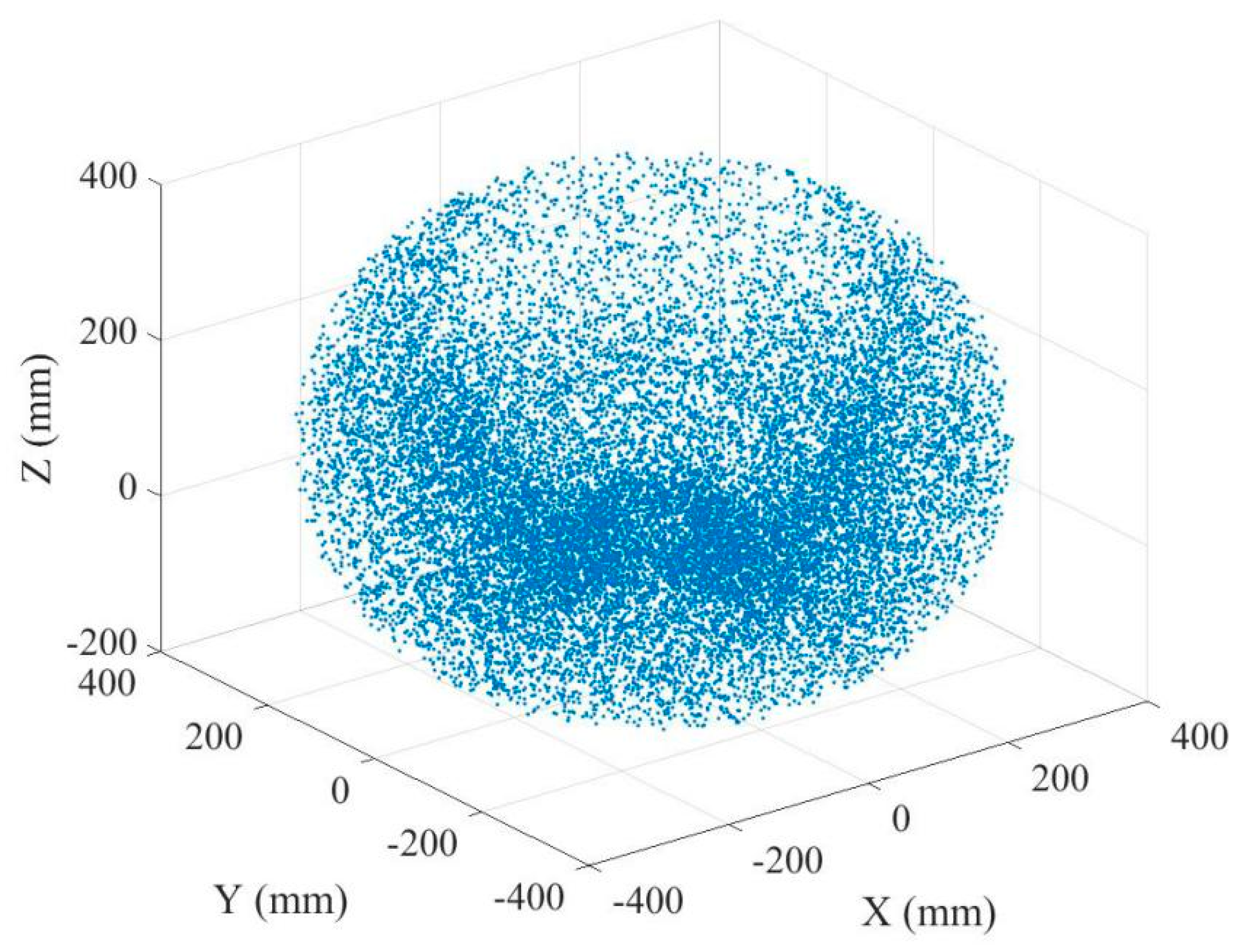
5.1. Verification of the Extraction of Workspace Boundary Based on 3D-Layering Concept

Figure 1 is a structural diagram of the modeled multijoint industrial robot for 3D printing. This position is its initial position. At this position, V_A = [–292.0, 0] mm, V_B = [−230.0, −76] mm, V_C = [−230.0, 79] mm, and V_W = [−292.0, −179] mm. In the experiment, V_U = [225, −70,12] mm. The range of joint angles is α ϵ [−180°, 180°], β ϵ [−40°, 100°], and γ ϵ [−150°, −55°]. According to Equation (30), f(−40°, −150°) = −34.6246 mm, f(−40°, −55°) = −175.9471 mm, f(100°, −150°) = 117.7572 mm, and f(100°, −55°) = 382.9244 mm. Thus, the maximum of Z is 382.9244 mm, and the minimum is −175.9471 mm. The contour boundary in Equation (31) was imported into the modeling software to generate a 3D printing layering model of the entire workspace, as shown in Figure 9. The layer height was then set to 0.2mm and the 3D-printing codes for the entire workspace were exported for physical printing of the workspace. From the 3D-printing layering model, the boundary curves of each layer were obtained in the entire workspace, as shown in Figure 10 and Figure 11.

As in Section 4.1, in order to compare with other methods, especially the Monte Carlo method, the boundary curve of the workspace when P_z = 200 mm was extracted using the method in this paper, as shown in Figure 12. By comparing Figure 12 with Figure 7, it was observed that the boundary curve of the workspace extracted by Monte Carlo method was irregular, which affected the accuracy and efficiency of the solution of the workspace. The boundary curve extracted by the method proposed in this paper was closer to the real boundary and had a better fitting degree and smoothness compared to the actual workspace.

5.2. Verification of Multisolution Selection Method Based on the Key Degrees of the Joints

In order to verify the correctness of the multisolution selection method based on the key degrees of the joints, the workspace stratification model generated in Section 5.1 was used to select a layer boundary for analysis. As shown in Figure 12, two path points P₀ = (258.238, 12.483,200) and P₁ = (255.829, 37.333, 200) were taken from the printing path, and Q₀ = (2.7675, 99.0989, −117.2417) was known. Verification of the multisolution selection method was performed according to the following steps.

(1)

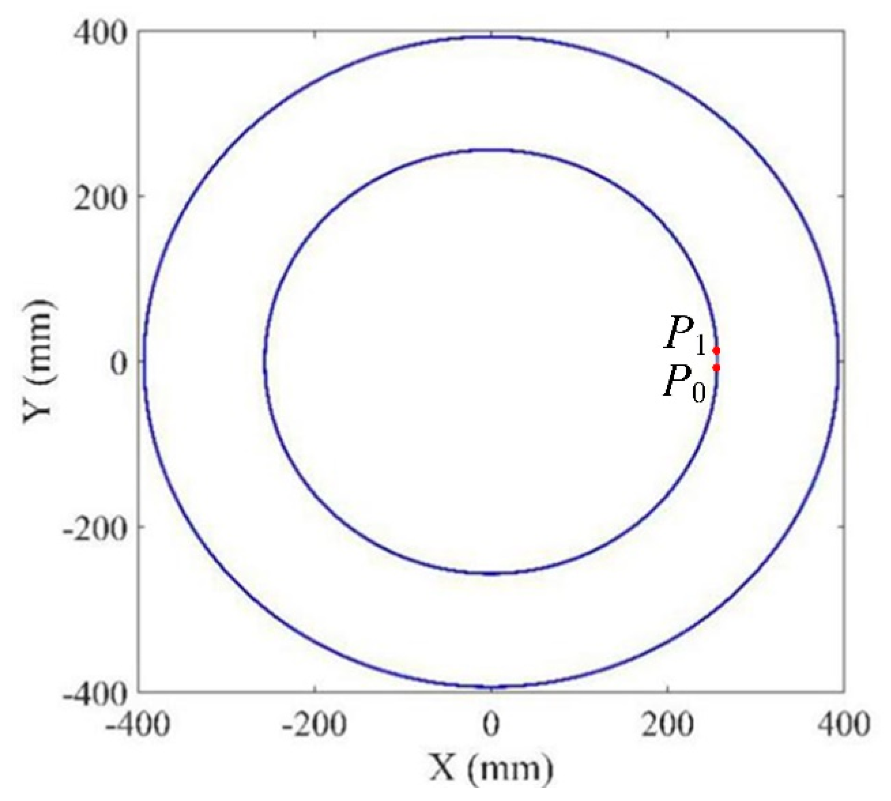
According to the inverse kinematic formula in Section 2.2, four groups of solutions of joint angles at path point P₁ were solved, and then all possible groups of joint angles were obtained according to Equation (12), as shown in

Table 4. Four groups of solutions at P₁ (unit: degree).

Num.	α (qθ1,1) (°)	β (qθ2,1) (°)	γ (qθ2,1) (°)
1Q1	8.3025	99.0992	−117.2420
2Q1	8.3025	−32.0948	117.2420
3Q1	−171.6975	99.0992	−117.2420
4Q1	−171.6975	−32.0948	117.2420

. They were seen as the possible solutions for the 0th key joint.

(2)

According to Section 3.1, the Jacobian matrix J₀ was obtainedat the path point P₀. The sensitivity S_q of each joint was calculated by the Jacobian matrix J₀.

$${\mathrm{J}}_0=\left[\begin{array}{ccc}98.7823& -34.0912& 108.8027\\ -251.6241& -13.3835& 42.7137\\ 0& 158.3195& 136.8850\end{array}\right]$$

$$\{\begin{array}{l}{\mathrm{S}}_{\mathrm{\alpha }}=270.3195\\ {\mathrm{S}}_{\mathsf{\beta }}=162.5004\\ {\mathrm{S}}_{\mathsf{\gamma }}=180.0000\end{array}$$

The key degrees of all joints were obtained and all joints were sorted according to their sensitivity. For S_α > S_γ > S_β, the A-joint was the first key joint and its key order was one; the C-joint was the second key joint and its key order was two; the B-joint was the third key joint and its key order was three.

The nominal increments and the nominal joint angles of all joints were calculated based on Equations (16) and (17) with the Jacobian matrix. The displacement components of the end position from the path point P₀ to P₁ were calculated as ΔP_x = −2.409 mm, ΔP_y = 24.850 mm, and ΔP_z = 0 mm. According to the Jacobian matrix J₀ and Equation (16), the nominal increments of all joint angles from P₀ to P₁ were calculated as

$$\mathrm{\Delta }{\mathrm{Q}}_1={\left[\mathrm{\Delta }{\mathrm{\alpha }}_1,\mathrm{\Delta }{\mathsf{\beta }}_1,\mathrm{\Delta }{\mathsf{\gamma }}_1\right]}^{\mathrm{T}}={\left({\mathrm{J}}_0{}^{\mathrm{T}}\cdot {\mathrm{J}}_0\right)}^{-1}\cdot {\mathrm{J}}_0{}^{\mathrm{T}}\cdot \left({\mathrm{P}}_1-{\mathrm{P}}_0\right)={\left[0.0965,0.0083,-0.0071\right]}^{\mathrm{T}}\mathrm{r}\mathrm{a}\mathrm{d}={\left[5.5264°,0.4766°,-0.4083°\right]}^{\mathrm{T}}$$

Based on Equation (17), the nominal joint angles ${\mathrm{Q}}_1^{\mathrm{n}}$ of point P₁ were obtained.

$${\mathrm{Q}}_1{}^{\mathrm{n}}={\mathrm{Q}}_0+\mathrm{\Delta }{\mathrm{Q}}_1={\left[\mathrm{\Delta }{\mathrm{\alpha }}_1{}^{\mathrm{n}},\mathrm{\Delta }{\mathsf{\beta }}_1{}^{\mathrm{n}},\mathrm{\Delta }{\mathsf{\gamma }}_1{}^{\mathrm{n}}\right]}^{\mathrm{T}}={\left[8.2939°,99.5755°,-117.6500°\right]}^{\mathrm{T}}$$

• For j = 1, the joint with the key order of 1 was found to be the A-joint. Its nominal joint angles ${\mathsf{\theta }}_{1,1}^{\mathrm{n}}$ were obtained as 8.2939° based on ${\mathrm{Q}}_1^{\mathrm{n}}$. The differences $\left|{}_{\mathrm{q}}{\mathsf{\theta }}_{1,1}-{\mathsf{\theta }}_{1,1}^{\mathrm{n}}\right|$ between ${\mathsf{\theta }}_{1,1}^{\mathrm{n}}$ and _qθ_1,1 in Table 4 were calculated. The smallest difference of α-joint angles was 8.3025°−8.2939°=0.0086°. The possible solutions for the first key order were ₁Q₁ and ₂Q₁, and then, j = j + 1 = 2. The second key order was the C-joint, and its nominal joint angles ${\mathsf{\theta }}_{3,1}^{\mathrm{n}}$ were obtained as −117.65°. The differences of ${\mathsf{\theta }}_{3,1}^{\mathrm{n}}$ were calculated with the joint angles of the C-joint in ₁Q₁ and ₂Q₁. The possible solutions for the second key order were ₁Q₁, which had the smallest difference of ${\mathsf{\theta }}_{3,1}^{\mathrm{n}}$. For the third key order, the nominal joint angles were ${\mathsf{\theta }}_{2,1}^{\mathrm{n}}$ = 99.5755 and the possible solution was also ₁Q₁. As a result, the appropriate solution of point P₁ was Q₁ = ₁Q₁ = [8.3025, 99.0992, −117.2420]^T.

5.3. Experiments

The printing code of the workspace was generated with the proposed kinematics model and the multisolution method by setting V_U = [0,0,0]T. The multijoint-industrial-robot-based 3D-printing system then printed its own workspace. The simulation are proposed with the printing code by setting the layer height as 10mm and 5mm, respectively as shown in Figure 13. It was found here that it was difficult to print the actual size of the workspace, because the end-effector approached singularities near the boundaries of its workspace, where it lost rigidity and precision. In addition, the layer height setting may make printing time be too long, which will waste time and printing materials.

The entire workspace was scaled by 10 times in equal proportion, so the robot could print its workspace. The origin of the base of the robot was chosen as the origin of the scaling, as shown in Figure 14. After scaling, the height dimensions became Z_max = 38.2924 mm and Z_min = −17.5947 mm. The total height was 55.8871 mm. For printing, the scaled workspace model was translated to the print platform, as shown in Figure 14. First, the model was translated from the origin of the base to the origin of the WCS with vector V_a = [225, −70,12]^T mm. At this time, the height of a part of the model was negative. The model was then translated with vector V_p = [70, 70, 5.5947]^T mm to make the model on the print platform. The printing code with joint angles of the robot was generated based on the model and the proposed multisolution method. Vector V_U = V_a + V_p was used for the calculation of the all possible joint-angle groups. With the printing code, the scaled workspace was printed with this multijoint robot. The printing material was PLA. The layer height was set to 0.2 mm, and feed velocity was 50 mm/min. The printed model of the scaled workspace is shown in Figure 15. The results showed that the workspace visualization method produced the real workspace, and the proposed kinematics and multisolution method can be used for 3D printing with such a robot.

The proposed method can be used to obtain and visualize a detailed workspace of a multijoint industrial robot by using a 3D-printing layering concept. There are some possible industrial applications. For example, multijoint industrial robots play a great role in automatic production lines, such as in automation welding, automatic material delivery, and automatic assembly. Detailed workspace models of such robots can be a great help for the arrangement of the robots. The trajectory of the welding or the material delivery should be in the workspace of the robot. The workspace also provides a restricted area for path planning and reliable control of the robot in an automatic production line. In addition, multijoint industrial robots can be used for 3D printing to manufacture complex freeform surfaces. The visual workspace can help to determine and optimize the locations of the printed parts. The printing trajectories are also limited by the workspace of the robot.

6. Conclusions

In this paper, a workspace visualization method of multijoint industrial robot based on 3D layering concept is proposed. First, a kinematic model of a multijoint industrial robot is established based on POE theory. According to the periodicity of trigonometric function and the stroke range of joint angles, all possible joint-angle groups of one pose are presented in detail.

Secondly, a multisolution selection method based on the key order of the joint is proposed. According to the Jacobian matrix of the multijoint industrial robot, the sensitivity of each joint is calculated to determine the key degree of each joint. The key order of a joint with a higher key degree is lower. A principle based on the smallest nominal joint-angle difference is then established. The nominal increments and the nominal joint angles of all joints are calculated with the Jacobian matrix. The possible solutions for the joints with high key order are selected from the joints with low key order. The possible solutions for the joint with the highest key order are the appropriate joint-angle groups of the point.

Thirdly, a workspace visualization method based on a 3D-printing layering concept is proposed. The formula of each layer’s contours are derived from the forward kinematics of the robot. It was proven that each layer of the workspace is a circle or ring. According to the structural parameters and the stroke range of joint angle, the minimum and maximum of the radius are obtained. The height limitations of the workspace are obtained based on the forward kinematics. According to the method of boundary extraction, the array of the boundary path points is obtained. Based on the postprocessing method proposed in this paper, the array is coded to obtain the joint-angle code of the workspace, which can be used for direct 3D printing. Finally, in order to verify the effectiveness of the proposed visualization method, an experimental multijoint-industrial-robot 3D-printing platform was used to print the whole workspace.

References

1. Xu, D.; Calderon, C.A.A.; Gan, J.Q.; Hu, H. An analysis of the inverse kinematics for a 5-dof manipulator. Int. J. Autom. Comput. 2005, 2, 114–124. [Google Scholar] [CrossRef] [Green Version]
2. Iliukhin, V.N.; Mitkovskii, K.B.; Bizyanova, D.A.; Akopyan, A.A. The modeling of inverse kinematics for 5 dof manipulator. Procedia Eng. 2017, 176, 498–505. [Google Scholar] [CrossRef]
3. Lee, C.S.G.; Ziegler, M. Geometric approach in solving inverse kinematics of puma robots. IEEE Trans. Aerosp. Electron. Syst. 1984, 20, 695–706. [Google Scholar] [CrossRef]
4. Fu, G.; Fu, J.; Shen, H.; Xu, Y.; Jin, Y.A. Product-of-exponential formulas for precision enhancement of five-axis machine tools via geometric error modeling and compensation. Int. J. Adv. Manuf. Technol. 2015, 81, 289–305. [Google Scholar] [CrossRef]
5. Chen, Q.; Zhu, S.; Zhang, X. Improved inverse kinematics algorithm using screw theory for a six-dof robot manipulator. Int. J. Adv. Robot. Syst. 2015, 12, 140–148. [Google Scholar] [CrossRef]
6. Fu, G.; Gao, H.; Gu, T. A universal postprocessor of general table-tilting type of five-axis machine tools without rotational tool center point function for actual nc code generation. In Proceedings of the ASME 2018 13th International Manufacturing Science and Engineering Conference, College Station, TX, USA, 18–22 June 2018. [Google Scholar]
7. Fu, G.; Gong, H.; Fu, J.; Gao, H.; Deng, X. Geometric error contribution modeling and sensitivity evaluating for each axis of five-axis machine tools based on poe theory and transforming differential changes between coordinate frames. Int. J. Mach. Tools Manuf. 2019, 147, 103455. [Google Scholar] [CrossRef]
8. An, H.S.; Seo, T.W.; Lee, J.W. Generalized solution for a sub-problem of inverse kinematics based on product of exponential formula. J. Mech. Sci. Technol. 2018, 32, 2299–2307. [Google Scholar] [CrossRef]
9. Ayiz, C.; Kucuk, S. The kinematics of industrial robot manipulators based on the exponential rotational matrices. In Proceedings of the IEEE International Symposium on Industrial Electronics, Seoul, Korea, 5–8 July 2009. [Google Scholar]
10. Yahya, S.; Mohamed, H.A.F.; Moghavvemi, M.; Yang, S.S. A geometrical inverse kinematics method for hyper-redundant manipulators. In Proceedings of the 2008 10th Intl. Conf. on Control, Automation, Robotics and Vision 2008, Hanoi, Vietnam, 17–20 December 2008; pp. 1954–1958. [Google Scholar]
11. Ananthanarayanan, H.; Ordóñez, R. Real-time inverse kinematics of (2n+1) dof hyper-redundant manipulator arm via a combined numerical and analytical approach. Mech. Mach. Theory 2015, 91, 209–226. [Google Scholar] [CrossRef]
12. Beheshti, M.T.H.; Tehrani, A.K.; Ghanbari, B. An optimized adaptive fuzzy inverse kinematics solution for redundant manipulators. In Proceedings of the International Symposium on Intelligent Control 2003, Houston, TX, USA, 8 October 2003; pp. 924–929. [Google Scholar]
13. Ayyıldız, M.; Cetinkaya, K. Comparison of four different heuristic optimization algorithms for the inverse kinematics solution of a real 4-dof serial robot manipulator. Neural Comput. Appl. 2015, 27, 825–836. [Google Scholar] [CrossRef]
14. Guang, W.-D.; Yin, L.-Z.; Wei, S.-T. Inverse kinematics of robot based on weighted optimization. Modul. Mach. Tool Autom. Manuf. Tech. 2016, 5, 1–8. [Google Scholar]
15. Xiao, L.-G.; Feng, T.-R. Algorithm for the inverse kinematics calculation of 6-dof serial welding robots based on geometry. Mach. Des. Manuf. 2015, 2, 29–35. [Google Scholar]
16. Sen, D.; Singh, B.N. A geometric approach for determining inner and exterior boundaries of workspaces of planar manipulators. J. Mech. Des. 2008, 130, 022306. [Google Scholar] [CrossRef]
17. Abdel, K.-M.; Yang, J. Workspace boundaries of serial manipulators using manifold stratification. Int. J. Adv. Manuf. Technol. 2006, 28, 1211–1229. [Google Scholar] [CrossRef]
18. Wang, X.-Y.; Ding, Y.-M. Method for workspace calculation of 6r serial manipulator based on surface enveloping and overlaying. J. Shanghai Jiaotong Univ. Sci. 2010, 15, 556–562. [Google Scholar] [CrossRef]
19. Gan, Y.; Yu, W.; He, W.; Wang, J.; Sun, F. The research about prescribed workspace for optimal design of 6r robot. Mod. Mech. Eng. 2014, 4, 154–163. [Google Scholar] [CrossRef] [Green Version]
20. Liu, X.-J.; Jinsongwang, W.; Oh, K.-K.; Kim, J. A new approach to the design of a delta robot with a desiredworkspace. J. Intell. Robot. Syst. 2004, 39, 209–225. [Google Scholar] [CrossRef]
21. Bergamaschi, P.R.; Nogueira, A.C.; de Fátima Pereira Saramago, S. Design and optimization of 3r manipulators using the workspace features. Appl. Math. Comput. 2006, 172, 439–463. [Google Scholar] [CrossRef]
22. Kohli, D.; Spanos, J. Workspace analysis of mechanical manipulators using polynomial discriminants. J. Mech. Transm. Autom. Des. 1985, 107, 209–215. [Google Scholar] [CrossRef]
23. Kohli, D.; Hsu, M.-S. The jacobian analysis of workspaces of mechanical manipulators. Mech. Mach. Theory 1987, 22, 265–275. [Google Scholar] [CrossRef]
24. Yang, J.; Abdel-Malek, K.; Zhang, Y. On the workspace boundary determination of serial manipulators with non-unilateral constraints. Robot. Comput. -Integr. Manuf. 2008, 24, 60–76. [Google Scholar] [CrossRef]
25. Cao, Y.; Lu, K.; Li, X.; Zang, Y. Accurate numerical methods for computing 2d and 3d robot workspace. Int J. Adv. Robot. Syst. 2011, 8, 1–13. [Google Scholar] [CrossRef] [Green Version]
26. Peidró, A.; Reinoso, Ó.; Gil, A.; Marín, J.M.; Payá, L. An improved monte carlo method based on gaussian growth to calculate the workspace of robots. Eng. Appl. Artif. Intell. 2017, 64, 197–207. [Google Scholar] [CrossRef]
27. Liu, Z.; Liu, H.; Luo, Z.; Zhang, X. Improvement on monte carlo method for robot workspace determination. Trans. Chin. Soc. Agric. Mach. 2013, 44, 230–235. [Google Scholar]
28. Merlet, J.P. An Improved Design Algorithm Based on Interval Analysis for Spatial Parallel Manipulator with Specified Workspace. In Proceedings of the IEEE International Conference on Robotics & Automation, Seoul, Korea, 21–26 May 2001; pp. 1289–1294. [Google Scholar]
29. Chablat, D.; Wenger, P.; Merlet, J.P. Workspace Analysis of the Orthoglide Using Interval Analysis. In Advances in Robot Kinematics; Lenarcic, J., Thomas, F., Eds.; Springer: Dordrecht, The Netherlands, 2002. [Google Scholar]
30. Kaloorazi, M.H.F.; Masouleh, M.T.; Caro, S. Determining the Maximal Singularity-free Circle or Sphere of Parallel Mechanisms Using Interval Analysis. Robotica 2014, 34, 1–15. [Google Scholar] [CrossRef]
31. Viegas, C.; Daney, D.; Tavakoli, M.; de Almeida, T. Performance analysis and design of parallel kinematic machines using interval analysis. Mech. Mach. Theory 2017, 115, 218–236. [Google Scholar] [CrossRef] [Green Version]
32. Yi, C.; Xiujuan, L.; Yi, N.; Guanying, Y. Computation and geometrical error analysis of a 3d robot’s workspace. Mech. Sci. Technol. 2006, 25, 1458–1461. [Google Scholar]
Figure 1. The structural parameters of one multijoint industrial robot.
Applsci 10 05241 g001
Figure 2. The kinematic chain of the multijoint industrial robot.
Applsci 10 05241 g002
Figure 3. The curve of the tangent function when α is in the range of [−π, π].
Applsci 10 05241 g003
Figure 4. The flow chart of the multisolution selection method based on the key order of joints.
Applsci 10 05241 g004
Figure 5. Workspace point cloud.
Applsci 10 05241 g005
Figure 6. The point cloud in the XY plane.
Applsci 10 05241 g006
Figure 7. The boundary curve in the XY plane.
Applsci 10 05241 g007
Figure 8. Schematic diagram of the contour of the workspace in the XZ plane.
Applsci 10 05241 g008
Figure 9. The 3D-printing model of the entire workspace.
Applsci 10 05241 g009
Figure 10. 3D workspace composed of boundary curves (nine layers).
Applsci 10 05241 g010
Figure 11. 3D workspace composed of boundary curves (281 layers).
Applsci 10 05241 g011
Figure 12. The boundary extracted by the method in this paper.
Applsci 10 05241 g012
Figure 13. Workspace printing path: (a) setting the height to 10 mm; (b) set the height to 5 mm.
Applsci 10 05241 g013
Figure 14. The scaling and the translating of the workspace model for 3D printing.
Applsci 10 05241 g014
Figure 15. (a) The 3D-printing system robot; (b) a 3D-printed object of the workspace.
Applsci 10 05241 g015