Article

Electrocoagulation Based Chromium Removal Efficiency Classification Using Logistic Regression

1
IME Lab, Faculty of Science Hassan 2 University, Casablanca 20250, Morocco
2
Engineering Unit, Euro-Med Research Center, Euro-Med University, Fez 30050, Morocco
3
SIRC-LAGES, Electrical Engineering Department, Hassania School of Public Labors, Casablanca 20250, Morocco
*
Author to whom correspondence should be addressed.
Appl. Sci. 2020, 10(15), 5179; https://doi.org/10.3390/app10155179
Submission received: 2 June 2020 / Revised: 11 July 2020 / Accepted: 17 July 2020 / Published: 28 July 2020
(This article belongs to the Section Chemical and Molecular Sciences)

Abstract

:

Featured Application

The main application of the proposed work is predicting wether an electrocoagulation operation will be efficient or not before testing in the real world. This allows avoiding trials and errors in order to optimize the Chromium removal process cost.

Abstract

Surface treatment and tanning industries use huge quantities of heavy metals—especially Chromium (III) and (VI)—in their processes thanks to its physical proprieties. It is used in the composition of special steels and refractory alloys. By dint of using this metal, an enormous quantity of rejects is produced each year and discharged into the oceans. As this is very dangerous for our environment, it is very important to treat these discharges before getting rid of them. This study treats chromium removal as a special type of heavy metals that can be a component of industrial discharges. Electrocoagulation is considered among the best methods used in this kind of treatment. However, it requires a lot of time, energy and remains expensive. This paper presents a predictive model in order to classify the chromium removal efficiency using electrocoagulation method. The proposed model is a logistic regression (LR) that consumes four parameters that we call predictors: pH, time, current, and stirring speed. After the training and validation process, we obtained 88% as classification precision, recall and F-Score metrics values while the use of the 10-Folds cross-validation method gave a minimal area under curve (AUC) value of 97% while the best value attempts 100%. Classification report states that the model performs well comparing to similar experimentation efficiencies.

1. Introduction

Chromium is a widely used heavy metal in the surface treatment and tanneries industries due to its physical properties such as strength, hardness, and resistance to corrosion and oxidation capabilities. Consequently, large quantities of this metallic waste are produced every year and released in the environment. Chromium can exist in several chemical forms with degrees of oxidation ranging from 0 to VI but only the trivalent and hexavelant forms are the most stable in the environment [1]. Chromium (III) is necessary for the body but in limited quantities. The maximum allowable limit for total chromium in drinking water is from 50 ug/L to 100 ug/L [2]. It is involved in various biochemical reactions of carbohydrates and lipid metabolism. Excessive consumption of chromium (III) can also cause health problems as well as metabolic disorders in the case of diabetes. However, the hexavelant form of chromium: chromium (VI) is the most dangerous, even in small quantities. It has various health consequences, including allergic phenomena, skin rashes, stomach ulcers, and carcinogenic effects [3].
In view of the above, it is important to treat all this waste before getting rid of it. There are several techniques that are used such as chemical treatments by oxidation or physic-chemical treatments such as coagulation flocculation, membrane filtration, and ion exchange. Electrochemical methods such as electrocoagulation (EC) and electro-dialysis are used as well. Environmental issues about the chemical and biological contaminations of water have become a major concern for society and the paper [4] lists the advantages and disadvantages of techniques used for wastewater treatment. The majority of these treatments remain expensive. According to these constraints, we have proposed a statistical method which makes it possible to predict the experimentation efficiency class given the parameters that influence most the chromium removal using electrocoagulation. This helps to optimize the purification process without losing time and energy.

Understanding Electrocoagulation

Electrocoagulation is one of the widely used methods in the field of water treatment, which helps to remove heavy metals from water discharges. The authors of [5] studied the possibility of eliminating 5 different heavy metals in synthetic wastewater by electrocoagulation. They studied the impact of the various parameters (initial pH of the solution, current density, and initial concentration of the metal) involved in electrocoagulation. Obtained results state that all used metals—except the manganese—gave excellent elimination in the majority of the samples. The best elimination is obtained at a very high pH of 9, a current density of 6.25 mA/cm2 after 20 min for all the metal concentration. In the same topic, ref. [6] used principal component analysis (PCA) to evaluate the informational contribution of Electrocoagulation parameter to the removal efficiency. Authors—in [7]—analyzed the operating cost required to remove lead from industrial wastewater by studying the effect of the geometry of the electrodes. This study highlights, as a result, the effect of the geometry of the electrodes and their consumption as well as the energy consumption on the one hand and the value of the operating cost on the other hand. They found that the electric current supplied to the new electrode configuration. The duration of each experiment and the electrocoagulation treatment of the wastewater, has a direct effect on the cost of operation by adding to the other variables.
Electrocoagulation is a process that allows coagulating the pollutants thanks to an electrolysis with a Aluminium or Iron consumable anode. The electrocoagulation process creates, in the water to be treated, metallic cations or streams of metallic hydroxides. When a direct current is imposed between the anode and the cathode, an electric field occurs and induces numerous reactions. The main reactions that take place with the electrodes are: At the anode: It is the oxidation of a metal M that will pass from the solid state to the ionic state according to the reaction: M = M n + + n e . This chemical reaction—as shown in Equation (1)-can be accompanied by the formation of oxygen by electrolysis of water at high current densities:
2 H 2 O ( I ) = O 2 ( g ) + 4 H + ( a q ) + 4 e
At the cathode, the following water reaction occurs as shown in Equation (2). Electro-flotation of the flocs may occur following the release of H 2 and O 2 gases at both electrodes.
H 2 O + e = 1 2 H 2 + O H
It is also possible to use other metals as the soluble anode. Nevertheless, aluminum and iron remain the most used metals because of their affordable price and their ionic form which has a high valence. The quantity of material produced or consumed during an electrochemical reaction is calculated by Faraday’s law. It is a function of the duration of the operation and the Intensity of Current I. The quantity of metal m is given by the Faraday law given by the equation m = I . t . M n . F , with m is the mass of the dissolved metal or formed gas (g) and I represents the intensity of the imposed current (A), while t is electrolysis time. M stands to the molecular weight of the element under consideration (g/mol). F refers Faraday’s constant (96,500 C/mol) and finally n is the number of electrons involved in the reaction considered. If the electrolysis model comprises p electrodes, and is powered by a liquid with a flow Q e , then: C = m ( p 1 ) Q e , with C is the mass flow of dissolved metal (kg h/m3). Q e represents the flow rate of the cell (m3/h) and p is the number of electrodes. Finally m is the theoretical amount of dissolved metal (Kg). If other electrochemical reactions take place simultaneously, the electrolysis current will not be fully used by the oxidation reaction.

2. Related Works

Several authors used the logistic regression method and applied in several areas: ref. [8] used logistic regression and classification of three methods to analyze the severity of injuries caused by a motorcycle accident, based on very specific assumptions regarding the probability distribution, the Logit link function, and the classification tree as a non-parametric method that predicts the severity of injuries based on the set of predictors. According to [8] study, the best of the two models for predicting the severity of injuries in motorcyclists is binary logistic regression. The models worked similarly in terms of identified predictors. Then [9] used logistic regression and the carrier vector classification to predict a probability of failure associated with each sample of pipelines in water supply systems. The results obtained show that the logistic regression (LR) works slightly better than the classification of carrier vectors, and indicates that the number of unexpected failures could be considerably reduced. Others also used the logistic regression method [10] to assess the influence of several decision factors in order to provide mutual assistance in the event of a disaster in the electricity sector; ref. [11] to classify the image samples into two categories of non-refueling and refueling on the basis of ’a set of drawn extracts; ref. [12] to analyze and develop the failure modes of non-anchored atmospheric storage tanks suffering from floods and to develop configurable models of fragility and [13] to detect by logistic regression network failures. The main purpose of detecting network anomalies is to reliably identify malicious activity in traffic observations collected at specific monitoring points, to trigger alarms and to trigger responses in right time, likewise it is used to explain how to improve the cooler load distribution to reduce the energy consumption of the system. It has been proposed to control the system components with the trend of significant temperature variables to improve the sequencing of the coolers. The result indicates that this logistic regression method is more efficient in terms of the amount of information needed to predict decisions. Another statistical study and simulation of ocean current patterns using autoregressive logistic regression models was done by [14]. The results of this study show the effectiveness of the proposed statistical framework for analyzing the evolution of ocean current models. For example, there is an article [15] that makes a comparative study of Parkinson’s disease and selection features by logistic regression in DNA and the use of an alternative reduction approach with logistic regression. The same last method was used to reduce the number of entities and to create a classifier with a higher accuracy rate than all the entities. Also apply in water treatment, for instance there is an article [16] controlled total inorganic nitrogen in treated wastewater using non homogeneous Markov logistic and multinomial logistic regression models. The results of this study indicate that temperatures have been cooled, the total ammonia nitrogen (TAN) in the effluents and the TIN levels in the effluents from previous weeks predict the TIN concentrations in the effluents. Another application of logistic regression—as explained in [17]—is to reduce dimensions and solve multi-collinearity problems in cartography.
Chromium is a heavy metal that must be treated and removed in wastewater, and there are several articles that treat this metal in different ways and different treatment methods. For example, this article [18] made a comparison between coagulation and electrocoagulation using iron to treat the water contained in the aquifer contaminated by a relatively high concentration of total chromium. The results showed that more than 99% of (Cr) was eliminated by the Coagulation and Electrocoagulation methods. However, Coagulation increased the concentration of dissolved solids above the recommended recommendation for drinking water. Another article [19] described the potential role of various functional nano-materials in the treatment of (Cr) in an aqueous medium with regard to the key value of merits, such as the adsorption capacity, the elimination efficiency and the coefficient of sharing. The objective of this study is to determine the most effective and economical options for controlling (Cr) in the aquatic environment. Then, Electrodialysis was used as a sequential treatment of a hybrid anaerobic bio-reactor to assess the saturation of the flow of concentrated solution in its efficiency in order to remove chromium (VI) in anionic form ( C r 2 O 7 2 ) . The results showed that it is not possible to remove a concentrated solution of ( C r 2 O 7 2 ) ion even with clean membranes. As mentioned in [20], the concentration of the concentrated solution can be considered to be a limiting variable of the electrodialysis.

3. Materials and Methods

The aim of this section is to build a logistic regression model to classify-a posteriori-the efficiency of electrocoagulation method on the removal of Chromium in wastewater. That comes to establish a statistical association between the experience efficiency as an output and explanatory input variables: pH, time, current, and stirring speed. This method will help us find better experiences that will have an elimination rate greater than 80% given input setup values. In order to train the logistic model, we need to build a training data set. Details are given in the next subsection.

3.1. Labeled Dataset Building

Data used in this article are taken from [21]. The data table columns represents respectively the run number, conductivity, pH of the solution, the chromium concentration, the chromium removal rate, and experimentation efficiency class. This class is obtained by labeling (0) each elimination rate lower than 80% and (1) for each one with an efficiency of higher than 80%. Table 1 represents our learning data set:

3.2. Building Logistic Regression Model

3.2.1. Model Overview

Logistic regression is a binomial regression model, used to model the probability that a certain class or event occurs. The aim is to best build a simple mathematical model with numerous real observations, such as (yes) or (no) which is represented by an indicator variable where two values are labeled (0) and (1). In the logistic model, the log-odds represents the logarithm of the odds for the value labeled (1). It is a linear combination of one or more independent variables called predictors. The independent variables can be a binary variable (two classes, coded by an indicator variable) or a continuous variable (any real value). The corresponding probability of the value labeled (1) can vary between 0 and 1. Hence the labeling function converts log-odds to probability. The binary logistic regression model has two levels of the dependent variable: categorical outputs with more than two values are modeled by multi-nomial logistic regression, and the model itself simply models the probability of exit in terms of input. This function can be used to make a classifier by choosing a threshold value and classifying the entries with a higher probability than the threshold as a class and below the threshold like the other. This is a common way to create a binary classifier. Several fields use logistic regression, such as marketing, medicine, economics and social sciences. It helps these domains to make a prediction of events.

3.2.2. Logistic Model Building

Let us consider a logistic model with inputs-named predictors, x p H , x C D , and x C C that represent pH variable, Conductivity, and Concentration, respectively. The output is the probability that the experimentation will give attempted results with good efficiency which is represented by the event E = 1 . Let’s denote this possibility p ( E = 1 / X , Θ ) with X = ( x p H , , x C C ) and Θ = ( β 0 , , β 3 ) that represent the parameters set efficiency. We assume a linear relationship between the predictor variables and the log-odds of the event ( E = 1 ) . This linear relationship can be written in the following mathematical form (where l is the log-odds, b is the base of the logarithm, and β i are parameters of the model): l = log b ( p 1 p ) = β 0 + β 1 x p H + β 2 x C D + β 3 x C C . We can recover the odds by exponentiating the log-odds: p 1 p = b β 0 + β 1 x p H + β 2 x C D + β 3 x C C . By simple algebraic manipulation, the probability of the event ( E = 1 ) is given by Equation (3):
p = b β 0 + β 1 x p H + β 2 x C D + β 3 x C C b β 0 + β 1 x p H + β 2 x C D + β 3 x C C + 1 = 1 1 + b β 0 + β 1 x p H + β 2 x C D + β 3 x C C
The above formula shows that once β i are fixed, we can easily compute either the log-odds that E = 1 for a given observation, or the probability that E = 1 for a given observation. The main use-case of a logistic model is to be given an observation and estimate the probability p that ( E = 1 ) will occurs. In most applications, the base b of the logarithm is usually taken to be e 2 . 77 .

3.2.3. Logistic Model Fitting

Logistic regression is an important machine learning algorithm. The goal is to model the probability of a random variable E being 0 or 1 given experimental data x p H , x C D , . Consider a generalized linear model function parameterized by Θ = ( β 1 , β 2 , β 3 ) given by the equation: h Θ ( X ) = 1 1 + e Θ T X = p ( E = 1 | X ; Θ ) . Therefore, p ( E = 0 | X ; Θ ) = 1 h Θ ( X ) and since E { 0 , 1 } , we see that p ( E = e | X ; Θ ) is giving by: p ( E = e | X ; Θ ) = h Θ ( X ) e ( 1 h Θ ( X ) ) ( 1 e ) . Let’s suppose that we have done n electrocoagulation experimentation with the next configurations X 1 , , X n .
The log-likelihood function-given in Equation (4)—assuming that all the observations in the sample are independently Bernoulli distributed. Formally:
L ( Θ | X 1 , X n ) = log ( p ( E = 1 | X 1 , X n ; Θ ) )
= log i = 1 n p ( E = e i | X i ; Θ )
= i h Θ ( X i ) i e ( 1 h p ( X i ) ) ( 1 e i )
= log i = 1 n h Θ ( X i ) e i ( 1 h Θ ( X i ) ) ( 1 e i )
The regression coefficients are usually estimated using maximum likelihood estimation. Unlike linear regression with normally distributed residuals, it is not possible to find a closed-form expression for the coefficient values that maximize the likelihood function, so that an iterative process must be used instead; for example Newton’s method. This process begins with a tentative solution, revises it slightly to see if it can be improved, and repeats this revision until no more improvement is made, at which point the process is said to have converged. The optimization method Limited Memory Algorithm for Bound Constrained Optimization (LBFS)—described in [22]—is used and that gives good results.

4. Result and Discussion

4.1. Confusion Matrix

A confusion matrix, also called an error matrix, is a summary of the prediction results on a classification problem. The number of correct and incorrect predictions is summarized with count values and broken down by class. The confusion matrix shows the ways in which your classification model is confused when making predictions. It gives us an overview not only of the mistakes made by a classifier, but especially of the types of mistakes that are made. Suppose that C 11 is the observation is positive that should be positive ( T P ) , while C 12 is the positive observation but predicted negative ( F P ) . The value C 21 is the negative observation that are predicted as negative ( T N ) , while C 22 is the negative observation, but predicted as positive ( F N ) . In our case, after predicting using built logistic model, we obtained C 11 = 5 , that means: 5 data points was positive and effectively we found them positive using our logistic classifier. The value C 12 = 1 , C 21 = 0 and C 11 = 13 . These values are rearranged in the confusion matrix bellow in Equation (8)
C = 5 1 0 13

4.2. Classification Report
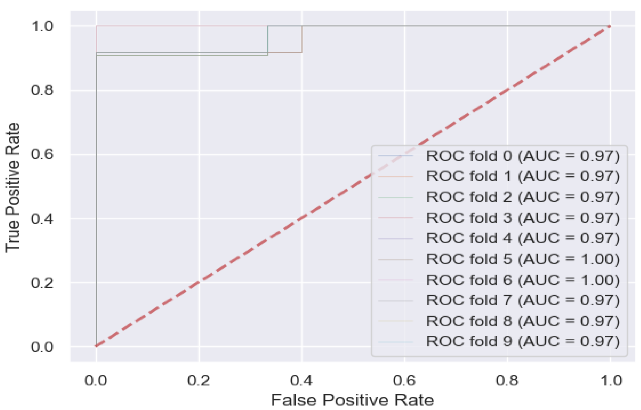
Let us start with the classification accuracy. It is a way to measure much a classifier performs. It can be called classification rate too and it is given formally by Equation (9):
A = T P + T N T P + T N + F P + F N
However, there are problems with accuracy. It assumes equal costs for both kinds of errors. A 99% accuracy can be excellent, good, mediocre, poor or terrible depending on the problem. For that reason, the use of other metrics seems to be necessary. Recall can be defined as the ratio of the total number of correctly classified positive examples divide to the total number of positive examples as in Equation (11). High recall indicates the class is correctly recognized (a small number of F N ).
R = T P T P + F N
Precision also is considered an important measure that complete the recall metric. To get the precision value, we divide the total number of correctly classified positive examples by the total number of predicted positive examples as in Equation (11). High Precision indicates an example labelled as positive is indeed positive (a small number of F P ).
P = T P T P + F P
High recall, low precision: This means that most of the positive examples are correctly recognized (low F N ) but there are a lot of false positives. However, low recall, high precision: This shows that we miss a lot of positive examples (high F N ) but those we predict as positive are indeed positive (low F P ). Since we have previously calculated the two measures : precision (P) and recall (R), it helps to have a measurement that represents both of them in one single metric. We calculate an F s c o r e that is a harmonic mean as it punishes the extreme values more. The F s c o r e —as defined in Equation (12)—will always be nearer to the smaller value of Precision or Recall.
F s c o r e = 2 . R . P R + P
Table 2 reports a summary of obtained results for each class.

4.3. ROC Curve

Figure 1 bellow is called (ROC curve) that stands for Receiver Operating Characteristic curve. It is a plot of the true positive rate against the false positive rate for the different possible ceil that is applied for the logistic regression to generate the predicted classes. It shows the tradeoff between sensitivity (given by T p / ( T p + F p ) ) in the Y axis and anti-specificity in the X axis (given by F p / ( T n + F p ) ). The closer the curve follows the top border and the left border, the more accurate the test. The area under the curve (AUC) measures of test accuracy. The ROC Curve is used to compare many classifiers: the best one is the one maximizing the (AUC) value. In this case, the 10-Folds cross-validation method is used to train and test the logistic regression model. Figure 1 show that the use of the 10-Folds cross-validation method gave a minimal area under curve value of 97% while the best values attempts 100% when is was tested on the 4 and 5 folds.

5. Conclusions

The objective of this work is to build a predictive model using logistic regression that will be used as an Electrocoagulation efficiency classifier. This model should be trained with collected data from laboratory experiments. The main application of the proposed work is predicting either an Electrocoagulation operation will be efficient or not before testing in real world. That allows avoiding trials and errors to optimize the Chromium removal process cost. Training and validation process gives 88% as classification precision, recall and F-Score metrics values while the use of the 10-Folds cross-validation method gave a minimal area under curve value of 97% while the best values attempts 100%. Classification report states that the model performs well comparing to similar experimentation efficiencies. As perspectives, the next works will broaden and generalize this approach. First, we will do our laboratory experiments with these and other parameters. Second, we apply this method to other heavy metals such as nickel, zinc, lead, etc. Then, we apply logistic regression to other chemical treatment methods such as membranes. We hope that the application of Statistics and Machine Learning for Chemistry helps to improve the field.

Author Contributions

Conceptualization, M.A., S.T., R.S. and A.T.; Methodology, M.A., S.T.; Software, S.T.; Validation, M.A., S.T., R.S., and A.T.; Formal analysis, M.A. and S.T.; Investigation, M.A.; Resources, M.A., S.T. and R.S.; Data curation, M.A. and S.T.; Writing original draft preparation, M.A.; Writing review and editing, M.A.; Visualization, S.T.; Supervision, R.S. and A.T.; Project administration, S.T., R.S. and A.T. All authors have read and agreed to the published version of the manuscript.

Funding

This research received no external funding.

Acknowledgments

I would like to thank the anonymous referees for their valuable comments and helpful suggestions. Special thanks goes to Hajar AKOULIH that improved the quality of the language and made this paper more readable.

Conflicts of Interest

The authors declare no conflict of interest.

Abbreviations

The following abbreviations are used in this manuscript:
ECElectrocoagulation
CrChromium
LRLogistic Regression
SVCClassification of Carrier Vectors
TANTotal Ammonia Nitrogen
TINTotal Inorganic Nitrogen
XWTCross-Wave Transformation

References

  1. Lunk, H.J. Discovery, properties and applications of chromium and its compounds. ChemTexts 2015, 1, 1–7. [Google Scholar] [CrossRef] [Green Version]
  2. Ivy, M.; Nadia, M.; Chad, S.; Chad, M.T. Hexavalent Chromium in Drinking Water. J. AWWA 2018, 110, 22–35. [Google Scholar] [CrossRef]
  3. Shahid, M.; Shamshad, S.; Rafiq, M.; Khalid, S.; Bibi, I.; Niazi, N.K.; Dumat, C.; Rashid, M.I. Chromium speciation, bioavailability, uptake, toxicity and detoxification in soil plant system: A review. Chemosphere 2017, 178, 513–533. [Google Scholar] [CrossRef] [PubMed]
  4. Grégorio Crini, E.L. Advantages and disadvantages of techniques used for wastewater treatment. Environ. Chem. Lett. 2018, 17, 145–155. [Google Scholar] [CrossRef]
  5. Pokhrel, N. Removal of Heavy Metals from Wastewater Using Electrocoagulation. Ph.D. Thesis, Metropolia Ammattikorkeakoulu, Helsinki, Finland, 2017. [Google Scholar]
  6. Akoulih, M.; Tigani, S.; Chaibi, H.; Saadane, R.; Tazi, A. Principal Component Analysis based Approach for Understanding Electrocoagulation Setting Impact on Chromium Elimination: A Step Toward Smart Eco-Friendly City. In Proceedings of the 4th International Conference on Smart City Applications (SCA’19), Casablanca, Morocco, 2–4 October 2019; pp. 1–6. [Google Scholar]
  7. ALJaberi, F.Y. Operating cost analysis of a concentric aluminium tubes electrodes electrocoagulation reactor. Heliyon 2019, 5. [Google Scholar] [CrossRef] [PubMed]
  8. Mahdi, R.; Amirarsalan Mehrara Molanb, K.K. Analyzing injury severity of motorcycle at-fault crashes using decision tree and logistic regression methods. Int. J. Transp. Sci. Technol. 2019. [Google Scholar] [CrossRef]
  9. Robles-Velasco, A.; Cortés, P.; Muñuzuri, J.; Onieva, L. Prediction of pipe failures in water supply networks using logistic regression and support vector classification. J. Pre-Proof 2019. [Google Scholar] [CrossRef]
  10. Wan, C.M.; Nosedal-Sanchez, A.; Nosedal-Sanchez, J.; Asgary, A.; Pantin, B. Modeling provision of disaster mutual assistance by electricity utilities using logistic regression. Int. J. Disaster Risk Reduct. 2019, 36, 891–921. [Google Scholar] [CrossRef]
  11. Nhat-Duc Hoang, Q.L.N.; Xuan-Linh, T. Automatic Detection of Concrete Spalling Using Piecewise Linear Stochastic Gradient Descent Logistic Regression and Image Texture Analysis. Complexity 2019, 2019, 14. [Google Scholar] [CrossRef] [Green Version]
  12. Yang, Y.; Chen, G.; Reniers, G. Vulnerability assessment of atmospheric storage tanks to floods based on logistic regression. Reliab. Eng. Syst. Saf. 2020, 196. [Google Scholar] [CrossRef]
  13. Palmieri, F. Network anomaly detection based on logistic regression of non linear chaoticin variants. J. Netw. Comput. Appl. 2019, 148, 102460. [Google Scholar] [CrossRef]
  14. Chiri, H.; Abascal, A.J.; Castanedo, S.; Antolínez, J.A.; Liu, Y.; Weisberg, R.H.; Medina, R. Statistical simulation of ocean current patterns using autoregressive logistic regression models: A case study in the Gulf of Mexico. Ocean. Model. 2019, 136, 1–12. [Google Scholar] [CrossRef]
  15. Kakade, A.; Kumari, B.; Dholaniya, P.S. Feature selection using Logistic Regression in Case–Control DNA methylation data of Parkinson’s disease: A Comparative study. J. Theor. Biol. 2018, 136. [Google Scholar] [CrossRef] [PubMed]
  16. Bihu, S.; Balaji Rajagopalan, J.S. Investigating regime shifts and the factors controlling Total Inorganic Nitrogen concentrations in treated wastewater using non-homogeneoues Hidden Markov and multinominal logistic regression models. Sci. Total Environ. 2019, 646, 625–633. [Google Scholar] [CrossRef]
  17. Sun, Q.; Zhang, P.; Wei, H.; Liu, A.; You, S.; Sun, D. Improved mapping and understanding of desert vegetation-habitat complexes from intraannual series of spectral endmember space using crosswavelet transform and logistic regression. Remote. Sens. Environ. 2020, 236. [Google Scholar] [CrossRef]
  18. Martín-Domínguez, A.; Rivera-Huerta, M.D.; Pérez-Castrejón, S.; Garrido-Hoyos, S.E.; Villegas-Mendoza, I.E.; Gelover-Santiago, S.L.; Drogui, P.; Buelna, G. Chromium removal from drinking water by redox-assisted coagulation: Chemical versus electrocoagulation. Sep. Purif. Technol. 2018, 130. [Google Scholar] [CrossRef] [Green Version]
  19. Maitlo, H.A.; Kim, K.H.; Kumar, V.; Kim, S.; Park, J.W. Nanomaterials based treatment options for chromiumin aqueous environments. Environ. Int. 2019, 130. [Google Scholar] [CrossRef] [PubMed]
  20. Dos Santos, C.S.; Reis, M.H.; Cardoso, V.L.; de Resende, M.M. Electrodialysis for removal of chromium (VI) from effluent: Analysis of concentrated solution saturation. J. Environ. Chem. Eng. 2019, 7. [Google Scholar] [CrossRef]
  21. Genawi, N.M.; Ibrahim, M.H.; El-Naas, M.H.; Alshaik, A.E. Chromium Removal from Tannery Wastewater by Electrocoagulation: Optimization and Sludge Characterization. Water 2020, 12, 1374. [Google Scholar] [CrossRef]
  22. Byrd, R.H.; Lu, P.; Nocedal, J.; Zhu, C. A Limited Memory Algorithm for Bound Constrained Optimization. J. Sci. Comput. 1995, 16, 1190–1208. [Google Scholar] [CrossRef]
Figure 1. Logistics Regression ROC Curve for every 10-Folds Cross-Validation Training Step.
Applsci 10 05179 g001
Table 1. Training Dataset.
RunCD (mA/cm2)pHConcentration (ppm)Removal (%)Class
120.04.001000.0071.400
220.09.01000.099.91
313.06.5750.098.51
413.06.51170.4584.60
56.04.0500.024.50
620.09.0500.095.01
713.06.5750.094.81
813.06.5750.094.61
913.010.7750.0100.01
1013.06.5750.094.61
1113.06.5750.094.51
121.226.5750.023.30
1324.776.5750.093.01
146.04.01000.02.80
1513.06.5750.094.31
166.09.0500.086.00
1720.04.0500.092.51
1813.06.5329.5599.91
1913.02.29750.019.50
206.09.01000.090.01
Table 2. Classification Report Summary.
ClassPrecisionRecallF-Score
0.00.830.830.83
1.00.920.920.92
Average0.880.880.88

