Abstract
Plants are ubiquitous in human life. Recognizing an unknown plant by its leaf image quickly is a very interesting and challenging research. With the development of image processing and pattern recognition, plant recognition based on image processing has become possible. Bag of features (BOF) is one of the most powerful models for classification, which has been used for many projects and studies. Dual-output pulse-coupled neural network (DPCNN) has shown a good ability for texture features in image processing such as image segmentation. In this paper, a method based on BOF and DPCNN (BOF_DP) is proposed for leaf classification. BOF_DP achieved satisfactory results in many leaf image datasets. As it is hard to get a satisfactory effect on the large dataset by a single feature, a method (BOF_SC) improved from bag of contour fragments is used for shape feature extraction. BOF_DP and LDA (linear discriminant analysis) algorithms are, respectively, employed for textual feature extraction and reducing the feature dimensionality. Finally, both features are used for classification by a linear support vector machine (SVM), and the proposed method obtained higher accuracy on several typical leaf datasets than existing methods.
1. Introduction
The traditional plant classification method is mainly realized by artificial recognition, which has the disadvantages of being time-consuming, susceptible to subjective judgment, and low recognition accuracy, far from meeting the requirements for rapid and accurate plant identification. Therefore, the rapid and accurate identification of plants is very challenging and meaningful. Plant recognition has been a challenging study since early last century, and plants play an irreplaceable role in human life. In the last decades, many researchers have studied image processing and pattern recognition as well as paid extensive attention to plant recognition. They have used images of plant organs (e.g., leaf, flower, fruit, and bark) for plant recognition.
In fact, although the images of flower, fruit, and bark have been employed for plant recognition, they have low recognition rates. In addition, these organ images have some limits; for instance, the flowering period is short and the texture of bark is unstable. Compared with flower, fruit, and bark, leaf images can be collected easily during the year, and its shape and texture are also stable. Therefore, the leaf is used as one of the important features for identifying plants. Most methods for plant recognition based on image processing rely on leaf images. In other words, plant species are recognized by leaf recognition.
In pattern recognition, using shape, texture, and color features for classification has been widely used. Soumyabrata et al. [1] proposed an improved text-based classification method to improve the classification results by integrating color and texture information. In addition, different color components and other parameters were compared and evaluated. Kristin et al. [2] introduced pattern recognition and computer vision as well as the application of texture features and pattern recognition. However, most leaves have small inter-class color differences, and some leaves have large intra-class color differences. As illumination may be uneven under natural conditions, the color features will affect recognition results. Therefore, the proposed method uses shape and texture features, which are more robust.
Both shape and texture features are used for leaf recognition. In 2012, Kumar et al. designed a mobile application Leafsnap, where histograms of curvature over scale (HoCS) [3] as a single (shape) feature was employed for plant identification. Other shape features are also used for leaf recognition, such as centroid-contour distance (CCD) [4], aspect ratio [5], Hu invariant moments [6], polar Fourier transform (PFT) [6], inner distance shape context (IDSC) [7], sinuosity coefficients [8], multiscale region transform (MReT) [9], etc. However, some leaves from different kinds of plants are very similar; the shapes of those leaves even cannot be differentiated by the naked eye. Hence, it is reasonable to use both shape feature and texture feature for leaf recognition. The most commonly used texture features contain entropy sequence (EnS) [10], histogram of gradients (HOG) [11], Zernike moments [12], scale invariant feature transform (SIFT) [13,14], gray-level co-occurrence matrix (GLCM) [15], and local binary patterns (LBP) [15]. Fu et al. [16] proposed a hybrid framework for plant recognition with complicated background. They extracted the block LBP operators as the texture features and calculated the Fourier descriptors as the shape features. Saleem et al. [17] combined 11 shape features, 7 statistical features, and 5 vein features for leaf recognition. Chaki et al. [18] used Gabor filter and GLCM to model texture feature and used a set of curvelet transform coefficients together with invariant moments to capture shape feature. Shao [19] proposed a new manifold learning method, namely supervised global-locality preserving projection (SGLP), for plant leaf recognition. Chaki et al. [20] proposed a novel approach by using the combination of fuzzy-color and edge-texture histogram to recognize fragmented leaf images. Some features based on Gabor filters [21,22], fractal dimension [23], locality projection analysis (SLPA) [24], kernel based principal component analysis (KPCA) [25], bag of word (BOW) [22,26] and convolutional neural networks (CNN) [27] are also used for leaf recognition.
In this paper, a new leaf feature called BOF_DP based on dual-output pulse-coupled neural network (DPCNN) and BOF is proposed, and an improved shape context called BOF_SC is also used in our plant image recognition system. The rest of the paper is organized as follows. Section 2 briefly introduces some related basic theories, including DPCNN and BOF. Section 3 introduces the theories related to feature extraction. Section 4 introduces the details of our proposed recognition method. Section 5 presents some comparative experimental results on several representative leaf image datasets.
2. Theory for Plant Recognition
2.1. Dual-Output Pulse-Coupled Neural Network
DPCNN was proposed by Li for geometry-invariant texture retrieval in 2012 [28]. The structure of DPCNN model is shown in Figure 1.
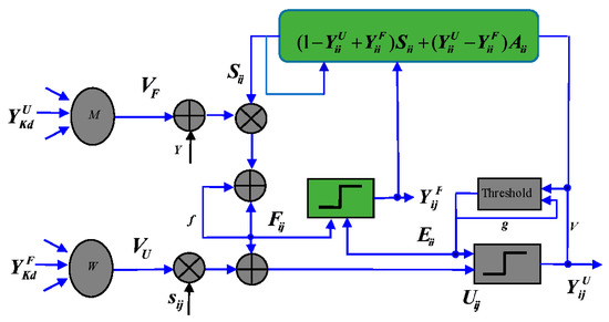
Figure 1.
Structure of DPCNN.
The mathematical expressions of DPCNN model are as follows:
where is the external stimulus, and it changes depending on the current outputs and . , , , , and are fixed constants between 0 and 1. and are the connection weights which the current neuron communicates with its neighbors. is the feeding out and is the compensating output.
Each neuron of DPCNN is an active neuron, which can be ignited by the feedback input or internal activity of the neuron to generate output pulse. First, the feedback input () changes due to the influence of external stimuli and external compensation output from neighboring neurons. Once the value of the feedback input () exceeds the active value, the neuron generates a feedback output pulse. Then, the feedback output, feedback input, and external stimulus from the neighboring neurons work together to change the value of the internal activity (). Once the value of the neuron’s internal activity item exceeds its activity threshold, a compensation output pulse is generated. Finally, the activity threshold () and external excitation () values are updated.
The pulse sequence generated by pulse-coupled neural network (PCNN) can represent the image edge and texture information; thus, it can extract effective image features. However, there are still some limitations in feature extraction. For example, there is only one pulse generator in the entire neuron model, and the excitation of neurons lacks a compensation mechanism. DPCNN is improved based on the PCNN model. Compared with PCNN, DPCNN has the following advantages: (1) each neuron of DPCNN has two chances to be excited; (2) DPCNN can adaptively change the size of the external excitation of each neuron; and (3) received local stimuli from peripheral neurons are affected by the modulation of the input stimulus. In addition, DPCNN also has translation, rotation, scale invariance, and robustness.
When DPCNN is used for feature extraction, the input image must be a gray image and the intensity of a pixel should be between 0 and 1. In our tests, the parameters were the same as in Ref. [28], except the iterations. The output of each iteration is a binary image, which is called pulse image. The entropy of the pulse image is used as a feature, and, after n times-iteration, the feature EnS, which is a vector with lengths of n, is obtained.
2.2. Bag of Feature
BOF model represents an image as an orderless collection of local features, and it has been widely used in pattern recognition. After the efforts of many researchers, the BOF model, which is used with spatial pyramid matching (SPM) [29] and locality-constrained linear coding (LLC) [30], has good performance in many studies. The flow chart of the BOF classification model is shown in Figure 2.
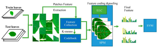
Figure 2.
BOF classification system.
LLC is a linear coding scheme with local constraints. Local constraint makes coding results more accurate and acquires spare code, and it improves the speed of training and classification. The mathematical expression of LLC is as follows:
where is the feature descriptor set obtained after the origin image blocking; is the coding result of ; denotes the dot product operation; and is the Euclidean distance between and .
SPM is an algorithm of image matching, recognition, and classification using spatial pyramid, and it is a method for obtaining the spatial information of the image by statistically distributing image feature points on images of different resolutions. Generally, it has two steps:
- (1)
- Extract features from different scales and combine them together.
- (2)
- Convert features of different lengths into fixed-length features.
When BOF works, each image of the dataset is divided into many blocks, and the size of the block is always 8 × 8. To get a better effect, neighboring blocks are combined as a patch. The collection of patches can be regarded as a bag of components. Generally, the sizes of the patches of the collection are too big, and many patches are similar. Thus, it is reasonable to unify similar patches into a standard component. In fact, the above operation is calculated in feature space such as SIFT space and HOG space. Patches are expressed by feature extracted from themselves; the collection of standard components counted by K-means is called codebook; and the standard component is called code. For each patch, it is described by its neighborhood (the code in codebook) using a histogram which is the function of LLC. Finally, the histogram is pooling by SPM, and the sparse and smooth feature is obtained.
3. Feature Extraction
3.1. Dictionary Learning
As traditional method of learning codebook is based on the unsupervised learning method K-means, which does not take advantage of training label. When K-means works to find the center of clustering, it will calculate the distances between a center and all the points; however, there are only a few parts of points which contribute to the calculation of center. Each cluster center is regarded as a visual vocabulary in the dictionary. When the dataset is large, it will cost a large amount of time and computing resource. The cost of clustering is mainly determined by the size of the feature matrix, and normally the size of the feature matrix is large. The features of the training set are employed to reduce the number of points while finding effective centers. For each species, D centers are counted; its typical value is 8. Combine the cluster centers of each class to get a dimensional dictionary, where is the number of species. If the value of the clustering center is too small, the features cannot be accurately clustered, and the error is large. However, if the value of the clustering center is too large, it will increase the calculation amount and time consumption. Therefore, the cluster center value we choose can reduce the learning cost and improve the learning speed.
3.2. Shape Feature Extractions
The shape of leaf is a basic feature of leaf image; when people identify an object, its shape comes to our mind firstly. Similarly, for leaf image recognition, the shape is a simple and fast feature, but the effect of a feature may be not qualified for leaf recognition by itself, as many kinds of leaf images have similar shapes. Thus, in our system, shape feature is a minor feature. As shown in Figure 3, after getting the contour of leaf image, the contour is cut into numerous shape fragments; the middle points of each fragment are shown in Figure 3C.
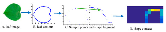
Figure 3.
SC acquisition.
Then, shape context is used as a descriptor of each fragment. Finally, the BOF model is used for feature coding and pooling so that we can get a more effective feature. Unlike bag of contour fragments (BCF), in this paper, uniform sampling method and simple fragments are used to improve the speed for feature classification.
3.3. Texture Feature Extractions
When DPCNN works, the parameters must be set firstly; the parameters of DPCNN in this paper are from Ref. [28], except the times of iteration. In our method, the image is divided into many blocks with 8 × 8 sizes (assuming that the number of patches is N to each kind of leaf images), each block is regarded as a patch. Then, after the iteration of n times, there will be n entropy images, and the entropy of each patch in every entropy image will be counted in order, as shown in Figure 4. If the entropy of one patch is ei, the entropy vector of the jth patch will be Ej = [e1, e2…… en]. To a species, the features matrix will be ENn, and eight codes (center of clustering) will be counted based on this matrix too.
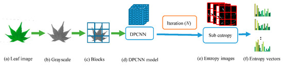
Figure 4.
Flow of getting entropy vector.
The process of extracting leaf image features by BOF_DPCNN combining DPCNN and BOF model is mainly divided into four stages: preprocessing, acquisition of DPCNN pulse images, low-level feature extraction, and feature coding. The process of obtaining image features of BOF_DPCNN is shown in Figure 4 and Figure 5. Since the datasets we used are processed, the preprocessing stage can be ignored. As shown in Figure 4, the color image is converted to grayscale image firstly, and then the grayscale image is divided into blocks of the same size. For each small block, the DPCNN model is iterated to obtain the pulse entropy images. Finally, the entropy vectors are calculated from the entropy images to obtain low-level features. The BOF model is used to construct the codebook with low-dimensional features, LLC is used to encode, and SPM is used for pooling, as shown as Figure 5.
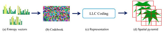
Figure 5.
Acquisition of image features using BOF_DPCNN: (a) entropy vectors obtained by DPCNN model; (b) codebook obtained by learning features; (c) the LLC coding; and (d) SPM for pooling.
4. Proposed Recognition Method
Image recognition has a fixed framework. In general, for plant recognition, object images acquired by special devices (e.g., camera or scanner) are used. In this paper, we select the leaf datasets with clean background for identification. Some key features which can identify the object are extracted from the images through various algorithms. The classifier is employed for classification after feature extraction. Most classifiers need to be trained by samples before classification. Finally, the result is obtained. The proposed method of leaf image recognition also adopts the above framework. The detailed scheme of the proposed method is shown in Figure 6. It can be divided into three steps: leaf image preprocessing, leaf feature extraction, and recognition. These steps are explained in the following.
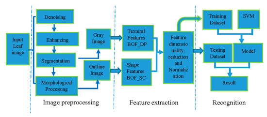
Figure 6.
Scheme of the proposed method.
4.1. Image Preprocessing
The leaf image is preprocessed to improve image quality. Image preprocessing contains the following steps.
- a.
- Image denoising: If the leaf image has some background information, the background should be deleted, which will decrease the calculations of features extraction. Because most leaf image datasets are built using optical scanners, the background is simple and easy to be removed by an adaptive threshold segmentation method.
- b.
- Image segmentation: Sometimes the obtained leaf image has a complex background, and it needs to be separated from the background by segmentation. Since most leaf images contain some regions without value, the target region is extracted by a morphology method. Then, a quadrilateral is used to surround the target region. The quadrilateral is obtained from the original image and rotated to horizontal.
- c.
- Image enhancement: Sometimes it is essential to enhance the contrast and texture of the image. Histogram equalization and linear stretching are adopted in this method. Then, high-pass filter is employed to enhance the edge and texture of the leaf image (gray image). Finally, texture feature is extracted from this gray image.
4.2. Feature Fusion
The feature extraction is introduced in Section 3. In this section, the two features are fused to a feature vector. Support F and T are the BOF_SC and BOF_DP features, respectively. Firstly, different weights α and β (support to α + β = 1) are assigned to F and T, thus the feature vector can be expressed as FV = [αF, βT]. The larger is the weight, the greater is the role of the feature in the fused feature. Because these weights greatly influence the final recognition result, α and β are usually determined after many experiments. As F and T are sparse matrices, FV is still a sparse matrix; it might be easy for classification, but it requires much memory. Thus, a direct linear discriminant analysis (LDA) algorithm [31] is used for dimensionality reduction. Finally, the final dimensionality of the feature vector is 1000.
4.3. Classification
There are many classifiers for leaf recognition, such as support vector machine (SVM) [10], probabilistic neural network (PNN) [5], K nearest neighbor (KNN) [32], and random forests [33]. The most commonly used is SVM for its high accuracy and easy of use. Liblinear [34] and Libsvm [35] are two popular SVM tools for classification. Although Libsvm and Liblinear can achieve similar results in linear classification, Liblinear is much more efficient than Libsvm in both training and prediction. When the number of samples is large, Liblinear is significantly faster than Libsvm [36]. Thus, we use Liblinear rather than Libsvm. Given a set of training leaf features Fvi, yi [1, …, N], where N is the number of leaf species, when Liblinear is used for leaf recognition, the problem can be defined as:
When Liblinear works, it will learn a multi-class space. ri represents the ith class learned from training data. In Equation (9), the first part is a linear regularization term or linear kernel. c is the weight of linear kernel. For the testing data, the predicted labels are defined by Equation (10).
5. Experiments and Analysis
5.1. Datasets
As leaf recognition becomes more and more attractive, many open source leaf datasets can be used for studies, such as Flavia [5], ICL [37], Swedish [38,39], MEW2012 [32], and so on.
Flavia dataset (http://flavia.sourceforge.net/) contains 1907 leaf images of 32 kinds, and it is the most used dataset for leaf recognition. Most leaves of Flavia dataset, as shown in Figure 7, are common plants in the Yangtze Delta, China. To each species, there are at least 50 leaves, which is enough for training and testing. These leaves are single leaves with the petiole removed and without complex background.
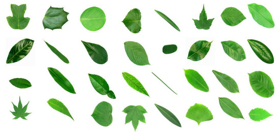
Figure 7.
Standard leaf image of Flavia dataset.
The ICL dataset (http://www.intelengine.cn/English/dataset) is collected by the Intelligent Computing Laboratory of the Chinese Academy of Sciences. The database contains 16,848 leaf images from 220 plants, with a different number of leaf images for each species. Some examples are shown in Figure 8.
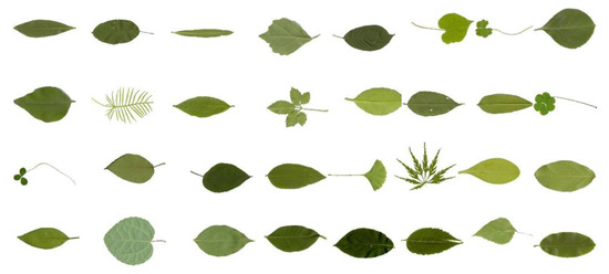
Figure 8.
Standard leaf image of ICL dataset.
The Swedish leaf dataset (http://www.cvl.isy.liu.se/en/research/datasets/sw) contains leaf images of 15 species each with 75 samples, for a total of 1125 Swedish leaf images. Figure 9 shows some example leaf samples of the Swedish dataset.
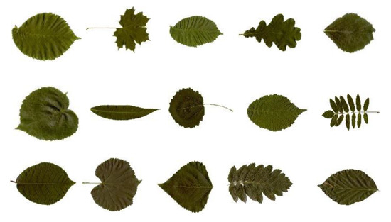
Figure 9.
Standard leaf image of Swedish dataset.
The MEW (Middle European Woods) dataset is a large dataset containing 153 species of Central European woody plants with a total of 9745 samples. Some examples are shown in Figure 10.
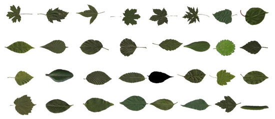
Figure 10.
Standard leaf image of MEW dataset.
5.2. Length of DPCNN
When DPCNN works, the iteration is a significant parameter which would influence the effect of features. In Ref. [28], the iteration is set at 47. Generally, for most all PCNN models, e.g., ICM and SCM, used for feature extraction, iterations are more than 30. To some degree, the iterative process is a process of feature extraction by using a dynamic threshold, which is the most prominent feature of PCNN models.
While the iterative process is also essential for BOF_DP, how much times it costs is the key point of this part. To find the best iteration of DPCNN, the iteration number was changed from 5 to 45 to find a better iteration below 45. In fact, if the iteration were 45 or more, the time for feature extraction would be too long, so the maximum of iteration was set at 45. On the other hand, for an image, the entropy vector is an approximate periodic vector; too many iterations would not be helpful, and, on the contrary, it would lower the feature’s productivity. Flavia dataset was selected for testing, where 30 sample images were selected for training for each species, and the remaining images were tested. The average recognition rates are listed in Figure 11. It is clear that the accuracy reaches its peak after a sharp increase. After the peak, when the iteration is 20, the accuracy shows a noticeable steady fall, and it never presents a rising trend. Hence, the best iteration number is around 20.
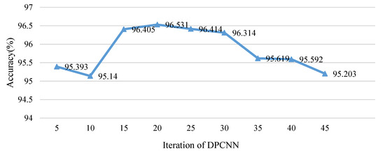
Figure 11.
Relationship between Iteration of DPCNN and accuracy.
BOF_DP has the best effect when iteration number is 20 while the traditional DPCNN has the best feature when the iteration number is 47. The iteration process is reduced obviously. To some extent, this may be caused by the method of sub-block processing, when images are divided into smaller pieces. The local feature is more outstanding in each block, but, when the iteration number is oversized, there would be some unnecessary data that can be regarded as noise. Actually, when the iteration number is smaller than 20, the redundancy and noise also exist. Hence, an effective method for feature selection will be helpful for improving the efficiency of the proposed feature.
5.3. Effect and Stability Analysis
The train number of each species (tr_no) was changed from 5 to 30 as shown in Figure 12. To each training set, SIFT with LLC coding was used for comparison, and the training set and testing set were kept the same for each feature. All the accuracies are the average of 10 times.
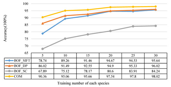
Figure 12.
The relationship between the training number of each species and the recognition accuracy.
It is obvious that, for each feature, the accuracy increases with tr_no. However, we are most concerned with the proposed feature BOF_DP showing a better effect than BOF_SIFT. Both BOF_SIFT and BOF_DP are better than BOF_SC, and the combined features of BOF_DP and BOF_SC achieved the highest recognition accuracy in the Flavia dataset.
To show the results of recognition clearly, recognition rates for each species are shown in Figure 13. The training number of each class was 30, and the final recognition rate on Flavia dataset was 98.2049%. Except for Species 11 and 25, the recognition accuracies of other species were ideal.
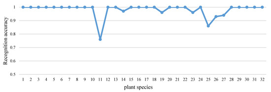
Figure 13.
The recognition accuracy of each species in the Flavia dataset.
5.4. Comparison of Features
Some other features were used for comparison, as shown in Table 1. BOF_DP represents the proposed feature, BOW + SIFT represents the features in Ref. [14], BOW + SC is also a proposed method based on SC and BOW in Ref. [14], LLC + SIFT is the original LLC method using SIFT [29], DBCS is a deformation-based representation space for curved shapes, and the authors of [39] proposed an adaptation of k-means clustering for shape analysis in DBCS. 2DPCA [40] is the 2D-based method of principal component analysis (PCA) and uses the bagging classifier with the decision tree as a weak learner. The recognition accuracies of these features are relatively close. 2DPCA has the lowest accuracy among these features. The proposed feature BOF_DP obtains the highest accuracy in the comparison.

Table 1.
Comparison of proposed feature with existing features on Flavia dataset.
5.5. Comparison of Different Methods
We also compared the proposed method with other methods on some datasets. To test the effectiveness and extensibility of the proposed feature and system, leaf datasets Flavia, ICL [37], Swedish [38,42], and MEW2012 [32] were used for testing.
As ICL contains so many leaf images, most methods always take a part of ICL dataset for testing. To compare with the MEW method [32], we followed its setting. On each dataset, for each species, half of leaf images were chosen as training sets, and the rest were the testing set. Supposing the number of species is p; if p is an even number, the training leaf images number was p/2; otherwise, the training leaf images number was (p + 1)/2. Finally, the training set and the testing set were roughly equal (in fact, the testing set was larger than the training set). The detailed data of the four datasets are shown in Table 2. In the following, all tests were repeated 10 times to get a convincing result.
Table 2.
Detail information of the four datasets.
First, we compared these methods on the Flavia dataset. The comparison results with other methods are shown in Table 3. ZRM [41] is a method based on Zernike moments. Z&H represents the method of Ref. [11], which is based on Zernike moments and histogram of oriented. VGG16 [42] and VGG19 [42] are the pre-trained models based on CNN architecture with logistic regression. MLAB (Margin, lobes, apex and base) [43] is the phenetic features of leaf. MLBP [44] is the method of extracting texture features based on modified local binary patterns. Muammer Turkoglu and Davut Hanbay [45] proposed the improved descriptors based on LBP, called region mean-LBP (RM-LBP), overall mean-LBP (OM-LBP), and ROM-LBP. RIWD (rotation invariant wavelet descriptor) [46] is a new shape proposed by Ehsan Yousefi et al. GIST [47] is an approach for plant recognition using GIST texture features. Wang et al. [48] proposed a few-shot learning method based on the Siamese network framework (S-Inception) to better classify the small sample size (where is the number of species used in this experiment and the number of trainings is 20). Most of these comparison methods do not introduce the number of training and test samples. Among the comparative methods, the deep learning-based method [42,48] does not obtain the best recognition results, but is slightly lower than other machine learning methods [44,45,46]. SSV [17] is a fusion feature composed of 11 shape features, 7 statistical features, and 5 vein features. The recognition result of SSV is slightly higher than our proposed method. As shown in Table 3, the training samples of the experiment are far more than the test sample images. It can be seen from the method Z&H [11] in Table 4 that, when the number of training samples increases and the number of test samples decreases, the recognition rate increases. Further, our method uses more total images than SSV. The total images of SSV were 1600, while our total images were 1907. More than 300 images were removed in SSV. The Flavia dataset we used is original and unfiltered. Therefore, it is understandable that the SSV method obtains a slightly better recognition rate under the very superior experimental conditions. Overall, the proposed method is superior to most of other existing methods.
Table 3.
Comparison of proposed method with existing methods on Flavia dataset.
Table 4.
Comparison of proposed method with existing methods on Swedish dataset.
Table 4 shows the results of different methods on the Swedish dataset. It contains 1125 sample images from 15 species, with 75 images per species. The authors of [49] proposed SMF, which utilizes the area ratio to quantify the convexity/concavity of each contour point at different scales to construct margin feature, and they used a combination of morphological features as shape feature. Yang et al. [50] introduced a novel multiscale Fourier descriptor (MF) based on triangular features, which effectively captures the local and global features of leaf shape. MARCH [51] (multiscale arch height) is a novel multiscale shape description. Wang et al. [52] proposed a hierarchical string cuts (HSCs) method. CSD [53] is a counting-based shape descriptor for leaf recognition, which can capture global and local shape information independently. CBOW is a shape recognition algorithm based on the curvature bag of words (CBOW) model. Generally, the recognition accuracy is improved with the increase of the number of training samples. When the training number of the method Z&H [11] is 750, the recognition result is significantly improved, which is slightly higher than the method we propose. In addition, compared with the other existing methods, the proposed method is superior. S-Inception [48] obtained the lowest recognition accuracy, while MEW [32], MF [50] and CSD [53] were close to the accuracy of the proposed method. The recognition accuracies of the other methods were also very close.
For ICL dataset, some researchers only use part of samples from dataset. Hence, the detailed comparisons are listed in Table 5. GTCLC [55] is a leaf classification method using multiple descriptors. Cem Kalyoncu et al. proposed a new local binary pattern (LBP) descriptor, and they combined it with geometric, shape, texture, and color features for leaf recognition. The authors of [56] used several different descriptors to extract texture and shape features and proposed a pre-training method based on the PID to improve the DBNs. DWSRC (discriminant WSRC) [57] is the method proposed by Zhang et al. for large-scale plant species recognition. The authors of [58] presented the novel relative sub-image sparse coefficient (RSSC) algorithm for mobile devices. DBNs chose 50 species for training and testing and it obtained the highest accuracy with 96%, higher than the proposed method; however, when the number of species in the experiment was 220, the recognition accuracy dropped to 93.90%. When 220 species were selected for training and testing, our proposed method achieved the highest accuracy 94.22%.
Table 5.
Comparison of proposed method with existing approaches on ICL dataset.
MEW dataset is also a large dataset. We compared our method with some classic methods, as shown in Table 6. The PCNN proposed by Wang et al. [59], based on pulse-coupled neural network and SVM, is a novel plant recognition method. PCNN and DPCNN have better performance than the others. It is obvious that the method we propose is better than the other methods.
Table 6.
Comparison of the proposed method with existing approaches on MEW dataset.
6. Conclusions
In this paper, we propose a new feature for plant recognition based on leaf image using DPCNN and BOF and propose a method combining BOF_SC and BOF_DP. In the proposed method, features of leaf are adopted, and SVM is taken as the classifier. Firstly, the proposed features BOF_DP were compared with the existing features on the Flavia dataset. After that, four famous leaf datasets were used to validate the performance of the proposed system. Experimental results show that BOF_DP has a better effect than other features, and our method is superior to other methods in recognition accuracy. However, to the DPCNN model, the parameters may not be optimal. In future work, we will try to find the best way to set the parameters automatically and improve the recognition accuracy.
Author Contributions
Writing—original draft preparation, Z.W. and J.C.; writing—review and editing, Z.W. and J.C.; project administration, Y.Z.; resources, J.K. and Y.M. All authors have read and agreed to the published version of the manuscript.
Funding
This study was jointly funded by China Postdoctoral Science Foundation (Grant No. 2013M532097), National Natural Science Foundation of China (Grant No. 61201421), the Foundation of National Glaciology Geocryology Desert Data Center (Grant No. Y929830201), and the 13th Five-year Informatization Plan of the Chinese Academy of Sciences(Grant No. XXH13506).
Conflicts of Interest
All Authors declare that they have no conflict of interest.
References
- Dev, S.; Lee, Y.H.; Winkler, S. Categorization of cloud image patches using an improved texton-based approach. In Proceedings of the 2015 IEEE International Conference on Image Processing (ICIP), Quebec City, QC, Canada, 27–30 September 2015; pp. 422–426. [Google Scholar]
- Kristin, J.D.; Gerard, M.; Sven, D. Computational Texture and Patterns: From Textons to Deep Learning. Synth. Lect. Comput. Vis. 2018, 8, 1–113. [Google Scholar]
- Kumar, N.; Belhumeur, P.N.; Biswas, A.; Jacobs, D.W.; Kress, W.J.; Lopez, I.C.; Soares, J.V.B. Leafsnap: A computer vision system for automatic plant species identification. In Proceedings of the European Conference on Computer Vision, Florence, Italy, 7 October 2012; pp. 502–516. [Google Scholar]
- Hasim, A.; Herdiyeni, Y.; Douady, S. Leaf Shape Recognition using Centroid Contour Distance. IOP Conf. Ser. Earth Environ. Sci. 2016, 31, 012002. [Google Scholar] [CrossRef]
- Wu, S.G.; Bao, F.S.; Xu, E.Y.; Wang, Y.-X.; Chang, Y.-F.; Xiang, Q.-L. A leaf recognition algorithm for plant classification using probabilistic neural network. In Proceedings of the 2007 IEEE International Symposium on Signal Processing and Information Technology, Cairo, Egypt, 15–18 December 2007; pp. 11–16. [Google Scholar]
- Singh, K.; Gupta, I.; Gupta, S. SVM-BDT PNN and Fourier moment technique for classification of leaf shape. Int. J. Signal Process. Image Process. Pattern Recognit. 2010, 3, 67–78. [Google Scholar]
- Ling, H.B.; Jacobs, D.W. Shape classification using the inner-distance. IEEE Trans. Pattern Anal 2007, 29, 286–299. [Google Scholar] [CrossRef]
- Kala, J.; Viriri, S. Plant specie classification using sinuosity coefficients of leaves. Image Anal. Stereol. 2018, 37, 119. [Google Scholar] [CrossRef]
- Yu, X.; Gao, Y.; Xiong, S.; Yuan, X. Multiscale Contour Steered Region Integral and Its Application for Cultivar Classification. IEEE Access 2019, 7, 69087–69100. [Google Scholar] [CrossRef]
- Wang, Z.; Sun, X.; Ma, Y.; Zhang, H.; Ma, Y.; Xie, W.; Zhang, Y. Plant recognition based on intersecting cortical model. In Proceedings of the 2014 International Joint Conference on Neural Networks (IJCNN), Beijing, China, 6–11 July 2014; pp. 975–980. [Google Scholar]
- Tsolakidis, D.G.; Kosmopoulos, D.I.; Papadourakis, G. Plant leaf recognition using Zernike moments and histogram of oriented gradients. In Proceedings of the Hellenic Conference on Artificial Intelligence, Ioannina, Greece, 15–17 May 2014; pp. 406–417. [Google Scholar]
- Kulkarni, A.H.; Rai, H.M.; Jahagirdar, K.A.; Upparamani, P.S. A leaf recognition technique for plant classification using RBPNN and Zernike moments. Int. J. Adv. Res. Comput. Commun. Eng. 2013, 2, 984–988. [Google Scholar]
- Nilsback, M.-E.; Zisserman, A. Automated flower classification over a large number of classes. In Proceedings of the Indian Conference on Computer Vision, Graphics & Image Processing, Bhubaneswar, India, 16–19 December 2008; pp. 722–729. [Google Scholar]
- Hsiao, J.-K.; Kang, L.-W.; Chang, C.-L.; Lin, C.-Y. Comparative study of leaf image recognition with a novel learning-based approach. In Proceedings of the IEEE Science and Information Conference, London, UK, 27–29 August 2014; pp. 389–393. [Google Scholar]
- Tang, Z.; Su, Y.; Er, M.J.; Qi, F.; Zhang, L.; Zhou, J. A local binary pattern based texture descriptors for classification of tea leaves. Neurocomputing 2015, 168, 1011–1023. [Google Scholar] [CrossRef]
- Fu, B.; Mao, M.; Zhao, X.; Shan, Z.; Yang, Z.; He, L.; Wang, Z. Recognition of Plants with Complicated Background by Leaf Features. J. Phys. Conf. Ser. 2019, 1176, 032053. [Google Scholar] [CrossRef]
- Saleem, G.; Akhtar, M.; Ahmed, N.; Qureshi, W.S. Automated analysis of visual leaf shape features for plant classification. Comput. Electron. Agric. 2019, 157, 270–280. [Google Scholar] [CrossRef]
- Chaki, J.; Parekh, R.; Bhattacharya, S. Plant leaf recognition using texture and shape features with neural classifiers. Pattern Recognit. Lett. 2015, 58, 61–68. [Google Scholar] [CrossRef]
- Shao, Y. Supervised global-locality preserving projection for plant leaf recognition. Comput. Electron. Agric. 2019, 158, 102–108. [Google Scholar] [CrossRef]
- Chaki, J.; Dey, N.; Moraru, L.; Fuqian, S. Fragmented plant leaf recognition: Bag-of-features, fuzzy-color and edge-texture histogram descriptors with multi-layer perceptron. Opt. Int. J. Light Electron Opt. 2019, 181, 639–650. [Google Scholar] [CrossRef]
- Lin, F.-Y.; Zheng, C.-H.; Wang, X.-F.; Man, Q.-K. Multiple classification of plant leaves based on gabor transform and lbp operator. In Proceedings of the International Conference on Intelligent Computing, Shanghai, China, 15–18 September 2008; pp. 432–439. [Google Scholar]
- Zheru, C.; Li, H.; Wang, C. Plant species recognition based on bark patterns using novel Gabor filter banks. In Proceedings of the International Conference on Neural Networks and Signal Processing, Nanjing, China, 14–17 December 2003; Volume 1032, pp. 1035–1038. [Google Scholar]
- Fuentes, S.; Hernández-Montes, E.; Escalona, J.M.; Bota, J.; Gonzalez Viejo, C.; Poblete-Echeverría, C.; Tongson, E.; Medrano, H. Automated grapevine cultivar classification based on machine learning using leaf morpho-colorimetry, fractal dimension and near-infrared spectroscopy parameters. Comput. Electron. Agric. 2018, 151, 311–318. [Google Scholar] [CrossRef]
- Zhang, S.W.; Lei, Y.K.; Dong, T.B.; Zhang, X.P. Label propagation based supervised locality projection analysis for plant leaf classification. Pattern Recogn 2013, 46, 1891–1897. [Google Scholar] [CrossRef]
- Valliammal, N.; Geethalakshmi, S. An optimal feature subset selection for leaf analysis. Int. J. Comput. Commun. Eng. 2012, 6, 440–445. [Google Scholar]
- Wang, X.G.; Feng, B.; Bai, X.; Liu, W.Y.; Latecki, L.J. Bag of contour fragments for robust shape classification. Pattern Recogn. 2014, 47, 2116–2125. [Google Scholar] [CrossRef]
- Nguyen Thanh, T.K.; Truong, Q.B.; Truong, Q.D.; Huynh Xuan, H. Depth Learning with Convolutional Neural Network for Leaves Classifier Based on Shape of Leaf Vein. In Proceedings of the Intelligent Information and Database Systems, Dong Hoi City, Vietnam, 19–21 March 2018; pp. 565–575. [Google Scholar]
- Li, X.J.; Ma, Y.D.; Wang, Z.B.; Yu, W.R. Geometry-Invariant Texture Retrieval Using a Dual-Output Pulse-Coupled Neural Network. Neural Comput 2012, 24, 194–216. [Google Scholar] [CrossRef]
- Lazebnik, S.; Schmid, C.; Ponce, J. Beyond bags of features: Spatial pyramid matching for recognizing natural scene categories. In Proceedings of the IEEE Computer Society Conference on Computer Vision & Pattern Recognition, New York, NY, USA, 17–22 June 2006; pp. 2169–2178. [Google Scholar]
- Wang, J.; Yang, J.; Yu, K.; Lv, F.; Huang, T.; Gong, Y. Locality-constrained linear coding for image classification. In Proceedings of the 2010 IEEE Conference on Computer Vision and Pattern Recognition (CVPR), San Francisco, CA, USA, 13–18 June 2010; pp. 3360–3367. [Google Scholar]
- Yu, H.; Yang, J. A direct LDA algorithm for high-dimensional data—With application to face recognition. Pattern Recogn. 2001, 34, 2067–2070. [Google Scholar] [CrossRef]
- Novotny, P.; Suk, T. Leaf recognition of woody species in Central Europe. Biosyst. Eng. 2013, 115, 444–452. [Google Scholar] [CrossRef]
- Hall, D.; McCool, C.; Dayoub, F.; Sunderhauf, N.; Upcroft, B. Evaluation of features for leaf classification in challenging conditions. In Proceedings of the IEEE Winter Conference on Applications of Computer Vision, Waikoloa, HI, USA, 5–9 January 2015; pp. 797–804. [Google Scholar]
- Fan, R.E.; Chang, K.W.; Hsieh, C.J.; Wang, X.R.; Lin, C.J. LIBLINEAR: A Library for Large Linear Classification. J. Mach. Learn Res. 2008, 9, 1871–1874. [Google Scholar]
- Chang, C.C.; Lin, C.J. LIBSVM: A Library for Support Vector Machines. Acm Trans. Intel. Syst. Tec. 2011, 2, 1–27. [Google Scholar] [CrossRef]
- Alvarsson, J.; Lampa, S.; Schaal, W.; Andersson, C.; Wikberg, J.E.; Spjuth, O. Large-scale ligand-based predictive modelling using support vector machines. J. Cheminformatics 2016, 8, 39. [Google Scholar] [CrossRef] [PubMed]
- Hu, R.X.; Jia, W.; Ling, H.B.; Huang, D.S. Multiscale Distance Matrix for Fast Plant Leaf Recognition. IEEE Trans. Image Process. 2012, 21, 4667–4672. [Google Scholar] [PubMed]
- Söderkvist, O. Computer vision classification of leaves from swedish trees. Master’s Thesis, Linkoping University, Linkoping, Sweden, 2001; p. 74. [Google Scholar]
- Demisse, G.G.; Aouada, D.; Ottersten, B. Deformation Based Curved Shape Representation. IEEE Trans. Pattern Anal. Mach. Intell. 2018, 40, 1338–1351. [Google Scholar] [CrossRef]
- Tharwat, A.; Gaber, T.; Hassanien, A.E. One-dimensional vs. two-dimensional based features: Plant identification approach. J. Appl. Log. 2017, 24, 15–31. [Google Scholar] [CrossRef]
- Kadir, A.; Nugroho, L.E.; Susanto, A.; Insap Santosa, P. Experiments of zernike moments for leaf identification. J. Theor. Appl. Inf. Technol. 2012, 41, 82–93. [Google Scholar]
- Pearline, A.; Kumar, S.; Harini, S. A study on plant recognition using conventional image processing and deep learning approaches. J. Intell. Fuzzy Syst. 2019, 36, 1997–2004. [Google Scholar] [CrossRef]
- Kolivand, H.; Bong, M.F.; Rahim, M.; Sulong, G.; Baker, T.; Tully, D. An expert botanical feature extraction technique based on phenetic features for identifying plant species. PLoS ONE 2018, 13, e0191447. [Google Scholar] [CrossRef]
- Naresh, Y.G.; Nagendraswamy, H.S. Classification of medicinal plants: An approach using modified LBP with symbolic representation. Neurocomputing 2016, 173, 1789–1797. [Google Scholar] [CrossRef]
- Turkoglu, M.; Hanbay, D. Leaf-based plant species recognition based on improved local binary pattern and extreme learning machine. Phys. A Statal Mech. Appl. 2019, 527, 121297. [Google Scholar] [CrossRef]
- Yousefi, E.; Baleghi, Y.; Sakhaei, S.M. Rotation invariant wavelet descriptors, a new set of features to enhance plant leaves classification. Comput. Electron. Agric. 2017, 140, 70–76. [Google Scholar] [CrossRef]
- Kheirkhah, F.M.; Asghari, H. Plant Leaf Classification Using GIST Texture Features. IET Comput. Vis. 2018, 13, 369–375. [Google Scholar] [CrossRef]
- Wang, B.; Wang, D. Plant Leaves Classification: A Few-Shot Learning Method Based on Siamese Network. IEEE Access 2019, 7, 151754–151763. [Google Scholar] [CrossRef]
- Zhang, X.; Zhao, W.; Luo, H.; Chen, L.; Peng, J.; Fan, J. Plant recognition via leaf shape and margin features. Multimed. Tools Appl. 2019, 78, 27463–27489. [Google Scholar] [CrossRef]
- Yang, C.; Yu, Q. Multiscale Fourier descriptor based on triangular features for shape retrieval. Signal Process. Image Commun. 2018, 71. [Google Scholar] [CrossRef]
- Wang, B.; Brown, D.; Gao, Y.; Salle, J.L. MARCH: Multiscale-arch-height description for mobile retrieval of leaf images. Inf. Sci. 2015, 302, 132–148. [Google Scholar] [CrossRef]
- Wang, B.; Gao, Y. Hierarchical String Cuts: A Translation, Rotation, Scale, and Mirror Invariant Descriptor for Fast Shape Retrieval. IEEE Trans. Image Process. Publ. IEEE Signal Process. Soc. 2014, 23. [Google Scholar] [CrossRef]
- Zhao, C.; Chan, S.S.F.; Cham, W.K.; Chu, L.M. Plant identification using leaf shapes—A pattern counting approach. Pattern Recognit. 2015, 48, 3203–3215. [Google Scholar] [CrossRef]
- Zeng, J.; Liu, M.; Fu, X.; Gu, R.; Leng, L. Curvature Bag of Words Model for Shape Recognition. IEEE Access 2019, 7, 57163–57171. [Google Scholar] [CrossRef]
- Kalyoncu, C.; Toygar, N. GTCLC: Leaf classification method using multiple descriptors. IET Comput. Vis. 2017, 10, 700–708. [Google Scholar] [CrossRef]
- Liu, N.; Kan, J.-M. Improved deep belief networks and multi-feature fusion for leaf identification. Neurocomputing 2016, 216, 460–467. [Google Scholar] [CrossRef]
- Zhang, S.; Zhang, C.; Zhu, Y.; You, Z. Discriminant WSRC for Large-Scale Plant Species Recognition. Comput. Intell. Neurosci. 2017, 2017. [Google Scholar] [CrossRef]
- Prasad, S.; Peddoju, S.K.; Ghosh, D. An adaptive plant leaf mobile informatics using RSSC. Multimed. Tools Appl. 2017, 76, 21339–21363. [Google Scholar] [CrossRef]
- Wang, Z.; Xiaoguang, S.; Zhang, Y.; Ying, Z.; Ma, Y. Leaf recognition based on PCNN. Neural Comput. Appl. 2015. [Google Scholar] [CrossRef]
© 2020 by the authors. Licensee MDPI, Basel, Switzerland. This article is an open access article distributed under the terms and conditions of the Creative Commons Attribution (CC BY) license (http://creativecommons.org/licenses/by/4.0/).