Abstract
Every day, hundreds of thousands of new malicious files are created. Existing pattern-based antivirus solutions have difficulty detecting these new malicious files. Artificial intelligence (AI)–based malware detection has been proposed to solve the problem; however, it takes a long time. Similarity hash–based detection has also been proposed; however, it has a low detection rate. To solve these problems, we propose k-nearest-neighbor (kNN) classification for malware detection with a vantage-point (VP) tree using a similarity hash. When we use kNN classification, we reduce the detection time by 67% and increase the detection rate by 25%. With a VP tree using a similarity hash, we reduce the similarity-hash search time by 20%.
1. Introduction
Every day, hundreds of thousands of new malicious files are created. [1] Existing pattern-based antivirus solutions have difficulty detecting these new malicious files because they do not contain patterns [2]. To solve these problems, artificial intelligence (AI)–based malware detection methods have been investigated [2,3,4,5,6,7,8,9].
AI-based malware detection consists of two phases. In the first phase, features are extracted from malicious files; in the second phase, a deep-learning model is trained using training data and tested using test data. Two methods are used to extract features from malicious files. The first is a static method that extracts opcodes from malicious files [3,4]. The second is a dynamic method that obtains application program interface (API) system-call sequences by running the malicious files in a sandbox [5,6,7].
Deep-learning models for malware detection include a convolutional neural network (CNN)-based model, a long short-term memory (LSTM)-based model, and a model using a CNN and LSTM together [9,10]. Deep-learning models have a high detection rate for malware detection. However, it takes a long time to determine whether or not files are malicious.
Other studies have investigated detecting malicious files using a similarity hash [7,11,12]. Trend Micro proposed Trend Micro locality-sensitive hashing (TLSH), which is a type of similarity hash. If a bit is changed in a file, its cryptographic hash, e.g., MD5, is completely different from the original hash. However, its similarity hash is quite similar to the original. Thus, when two similarity hashes are similar, the two files are similar. Similarity hash–based malware detection is faster than deep learning–based malware detection. However, its detection rate is lower.
In this paper, we propose two methods to solve these problems, as shown in Figure 1: k-nearest-neighbor (kNN) classification for malware detection and a vantage point (VP) tree using a similarity hash. First, using kNN classification for malware detection, we classify the training data into three groups, as follows.
{Normal group, malicious group, undecided group}
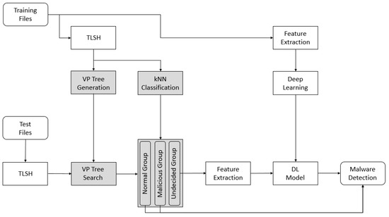
Figure 1.
Proposed system for fast malware detection. TLSH: Trend Micro locality-sensitive hashing. VP: vantage-point. kNN: k-nearest-neighbor. DL: deep learning.
kNN classification is used for malware detection to increase the detection rate of similarity hash–based malware detection and increase the speed of deep learning–based malware detection. In the normal group, each file and its kNN are normal files. In the malicious group, each file and its kNN are malicious files. The remaining files are in the undecided group. Thus, if a file in the undecided group is a normal file, its kNN is a malicious file, and if a file in the undecided group is a malicious file, its kNN is a normal file.
If the kNN of a new file is in the normal group, we can determine that it is a normal file. If its kNN is in the malicious group, we can determine that it is a malicious file by using a similarity hash. However, if its kNN is in the undecided group, we should determine whether or not the new file is malicious by using deep learning–based malware detection.
When a new file’s kNN is in the normal group or the malicious group, we can determine its type using only a similarity hash. Thus, we can reduce the malware-detection time compared to using only the deep learning–based method. Meanwhile, when a new file’s kNN is in the undecided group, we determine it using a deep learning–based model. Therefore, we can increase the detection rate compared to using only a similarity hash.
The second proposed method is a VP tree using a similarity hash. Even if similarity hash–based detection is faster than a deep learning–based method, it still takes a long time for many malicious files. At present, there are about 1 billion malicious files. [1] Therefore, we need to increase the speed of similarity-hash searches. Using a VP tree can accomplish this.
The proposed system works as follows. If training files are given, we compute similarity hashes, e.g., TLSH. Then, we generate a VP tree using the similarity hash and conduct a kNN classification. This classifies the training data into a normal group, a malicious group, and an undecided group. In addition, we extract features and train the deep-learning model for malware detection. Thus, we reduce the detection time, compared to using only the deep-learning model, by using kNN classification.
When a test file is provided, we compute a similarity hash and search the kNN using a VP tree. Then, if the kNN is in the normal group or malicious group, the file is determined to be normal or malicious, respectively. Otherwise, we extract the features from the test file and determine whether it is malicious or not using the deep-learning model. Thus, we increase the detection rate, compared to using only the similarity hash, by using the deep-learning model.
The contributions of this paper are as follows. First, by proposing the kNN classification for malware detection, we increase the malware detection rate compared with the similarity hash–based malware detection and reduce the detection time compared with deep learning–based malware detection. Second, by providing a VP tree, we reduce the search time of the similarity hash. Third, on conducting experiments about kNN classification and VP tree, we report that the malware detection rate is increased by 25%; the detection time is reduced by 67%; and the search time of the similarity hash is decreased by 20%.
This paper is organized as follows. In Section 2, we list related work. In Section 3, we introduce TLSH and the VP tree. In Section 4, we present kNN classification for malware detection and a VP tree using a similarity hash. In Section 5, we provide the experimental results. Finally, in Section 6, we conclude the paper.
2. Related Work
The methods used for analyzing malicious files can be categorized into static and dynamic analysis methods. The static analysis methods judge whether a file is malicious by analyzing strings, import tables, byte n-grams, and opcodes [13]. These methods can analyze malicious files relatively quickly, although they face difficulties analyzing files when the files are obfuscated or packed [14]. In contrast, using the dynamic analysis methods, malicious files are analyzed by running them. However, the disadvantage of these methods is that the malicious files may detect the virtual environment and not operate in it [3]. It may also be difficult to detect complete malicious behavior as malicious files may only run under specific circumstances.
Recently, there have been many studies on malicious file analysis using AI. The methods in [3,4] utilize a static analysis method to analyze malicious files. The method in [3] extracts byte histogram features, import features, string histogram features, and metadata features from a file and trains deep learning models based on deep neural networks. The method in [4] learns a CNN-based deep learning model [15] by extracting opcode sequences.
The approaches in [5,6,7] use a dynamic analysis method to analyze a malicious file, and then, execute the file to collect the API system call and extract a subsequence of a certain length from the system call sequence using a random projection. The method in [5] uses a deep neural network–based deep learning model, and that in [6] uses a deep learning model based on a recurrent neural network (RNN) [16]. The authors of [7] proposed a deep learning model that simultaneously performs malicious file detection and malicious file classification. The disadvantage of using deep learning for malware detection is that even if deep learning leads to a high detection rate, it still is time-consuming. To solve this problem, we propose using a kNN classification method for malware detection.
We focus on malicious portable executable (PE) files, but other types of malicious files also exist. These include malicious PDF files [17] and Powershell scripts [18,19]. Some researchers have attempted using AI to determine whether PDF files and Powershell scripts are malicious. However, such approaches are outside the scope of the present study.
In contrast, AI-based malware detection methods show good detection rates when a large volume of labeled data is available to run supervised learning. However, the lack of data can cause severe overfitting; further, collecting large quantities of malware is not easy. To solve this problem, the few-shot learning approach is proposed [20,21]. Using few-short learning, a model can learn general and high-level knowledge of malware from a few samples and adapt unseen classes during training. Few-shot learning is useful in the absence of a large volume of data. However, in this study, we assume that there are enough data to train the deep learning model for malware detection.
On the other hand, there are researches about evading malware detection using GAN [22,23,24,25]. They modify malware by using a generator to be detected as normal. Then, a discriminator cannot determine whether it is malicious. To solve this problem, we need various malware detection methods as well as AI-based malware detection.
Also, there are researches about AI-based intrusion detection as well as AI-based malware detection [26,27,28]. In [26], the proposed intrusion detection system (IDS) combines data analytics and statistical techniques with machine learning techniques to extract more optimized. In [27], when the number of abnormal connections is small, it may cause overfitting. To solve the problem, a resampling method is proposed. In [28], to evade intrusion detection, IDSGAN is proposed. However, intrusion detection is outside the scope of the present study.
Research on similarity hash–based malware detection has also been conducted [7,11,12]. Trend Micro proposed the Trend Micro locality-sensitive hash (TLSH) [11]. We can determine whether two files are similar by using TLSH. Unfortunately, fuzzy hash algorithms produce different similarity hashes when the input order differs. To solve this problem, Li et al. [12] proposed malware clustering, based on a new distance-computation algorithm. Huang et al. [7] extracted API system calls by running malicious files in the Cuckoo sandbox and computed similarity hashes using TLSH. Then, it classified the type of the malicious file by generating a distance matrix. However, the disadvantage of a similarity hash is its low detection rate. In this paper, we propose a method that increases the detection rate using kNN classification.
3. Preliminaries
In this section, we introduce two basic methods. First is TLSH, which is a type of similarity hash. Second is the VP tree, which rapidly finds the kNN.
3.1. TLSH
The purpose of a similarity hash is to find variants of a file. Hundreds of thousands of variant malicious files are created every day, which makes it difficult to detect them using existing pattern-based antivirus solutions. A similarity hash can help to solve this problem. When existing files are known to be normal or malicious, if a new file has similar similarity-hash values, it can be judged to be similar to an existing file.
The properties of the similarity hash are as follows. A cryptographic hash, e.g., MD5, produces a completely different hash value if the file is only slightly different. However, for similarity hashes, similar files have similar hash values and different files have different similarity-hash values.
TLSH is a typical example of a similarity hash [11]. A TLSH is created as follows. First, a byte string from the file is processed using a five-element sliding window to compute the bucket-count array. Second, quartile points , , and are calculated. Third, the digest header values are constructed. Fourth, the digest body is constructed by processing the bucket array.
First, as shown in Figure 2, a byte string of a file is counted into a 128-dimensional array using a Pearson hash [29]. That is, the value computed by the Pearson hash through a five-element window is matched to one of the 128 buckets and the bucket count is incremented by one.
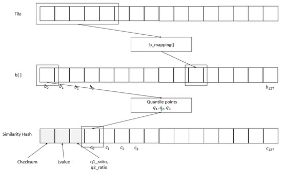
Figure 2.
TLSH.
Second, the quartile points are calculated. Seventy-five percent of the bucket counts are greater than or equal to , 50% of the bucket counts are greater than or equal to , and 25% of the bucket counts are greater than or equal to .
Third, as shown in Figure 2, the first byte of the first three bytes of the similarity hash is the checksum, the second byte is the length of the file, and the third byte is calculated from , and , as follows.
Finally, if the value of a bucket is less than or equal to , 00 is entered into . If the value is less than or equal to , 01 is entered. If it is less than or equal to , 10 is entered. Otherwise, 11 is entered. The TLSH is created through these four steps.
A method for calculating the similarity difference of two files using two similarity hashes is as follows. First, the difference between the similarity-hash header values is calculated. Second, the difference between the similarity-hash body values is calculated.
The difference in the header values of the similarity hash is calculated as follows.
Function distance_headers (tX, tY) {
ldiff = mod_diff (tX.lvalue, tY.lvalue, 256)
q1_diff = mod_diff (tX.q1_ratio, tY.q1_ratio, 16)
q2_diff = mod_diff (tX.q2_ratio, tY.q2_ratio, 16)
diff = ldiff × 12 + q1_diff × 12 + q2_diff × 12
if (tX.checksum! = tY.checksum) diff++
}
The difference in the body values of the similarity hash is calculated as follows.
Function distance_bodies (tX, tY) {
For i = 0 to 127 {
d = abs(x[i] − y[i])
if (d == 3) diff = diff + 6
else diff = diff + d
}
}
Finally, the difference between the two similarity-hash values is calculated as the sum of the difference between the similarity-hash header values and the difference between the similarity-hash body values.
3.2. VP Tree
The purpose of a VP tree [30] is to quickly find the kNN. The first step is the VP-tree generation and the second is the VP-tree search.
The VP tree is generated as follows. When there are many points, we select a vantage point (VP) randomly. Then, we compute the distances between the vantage point and the other points. We set the radius of the vantage point to the median of the distances. Then, we classify the points into two groups: inner and outer. The distance between the vantage point and a point in the inner group is less than the radius of the vantage point. The distance between the vantage point and a point in the outer group is greater than the radius of the vantage point. Then, the points in the inner group are assigned to the left subtree of the vantage point and the points in the outer group are assigned to the right subtree. Then, we recursively repeat this process in the subtree.
For example, we select as a vantage point, as shown in Figure 3. Then, we compute the distances between and the other points. We set the radius of to the median of the distances. Then, we classify the points into two groups.
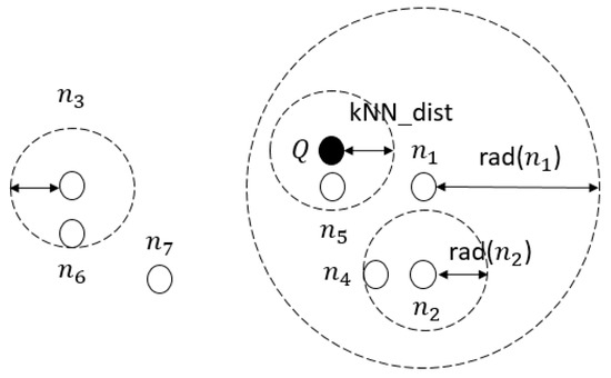
Figure 3.
VP-tree concept.
The points in the inner group are assigned to the left subtree of and the points in the outer group are assigned to the right subtree of , as shown in Figure 4.
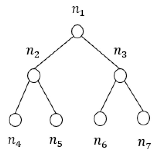
Figure 4.
VP-tree generation.
Next, in the subtree, we repeat this process recursively. In the left subtree, we select vantage point . Because the distance between and is less than the radius of , is assigned to the left subtree of . Because the distance between and is greater than the radius of , is assigned to the right subtree of .
In the right subtree, we select vantage point . Because the distance between and is less than the radius of , is assigned to the left subtree of . Because the distance between and is greater than the radius of , is assigned to the right subtree of .
Second, the VP tree is searched as follows. First, if the following condition is satisfied, the left subtree is pruned. This condition means that the points in the inner group of the vantage point are not within the distance of the kNN.
Second, if the following condition is satisfied, the right subtree is pruned. This condition means that the points in the outer group of the vantage point are not within the distance of the kNN.
Thus, by using the VP tree, we can quickly find the kNN.
For example, when a query point Q is given, as shown in Figure 3, because the distance between Q and vantage point is less than the difference between the radius of vantage point and the kNN distance, the right subtree of is pruned. This means that the points in the right subtree of are not kNNs of Q. Thus, , , and are pruned.
Next, in the left subtree of , the left subtree of is pruned because the distance between Q and vantage point is greater than the sum of the radius of vantage point and the kNN distance. This means that the points in the left subtree of are not kNNs of Q. Thus, is pruned. Finally, is the kNN of Q.
4. Proposed Method
The disadvantage of deep learning–based malware detection is that it takes a long time, and the disadvantage of similarity hash–based malware detection is its low detection rate. In Section 4.1, we propose the kNN classification method for fast malware detection. In Section 4.2, we provide a fast search method for the similarity hash.
4.1. kNN Classification Method for Fast Malware Detection
The disadvantage of similarity hash–based malware detection is its low detection rate. This means that the first nearest neighbor (1NN) of a normal file can be a malicious file or the 1NN of a malicious file can be a normal file. Therefore, we classify the training data into three groups in Figure 5: Normal, malicious, and undecided. In the normal group, each file is normal and its 1NN is also normal. In the malicious group, each file is malicious and its 1NN is also malicious. In the undecided group, if a file is normal, its 1NN is malicious and if a file is malicious, its 1NN is normal.
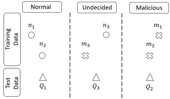
Figure 5.
kNN classification for fast malware detection.
The purpose of 1NN classification is to improve the malware detection speed and increase the detection rate. Given a test file , if its 1NN is in the normal group, we determine that is normal. If the 1NN of is in the malicious group, we determine that it is malicious. However, because the 1NN of is in the undecided group, we cannot determine whether it is malicious. Therefore, to determine if it is malicious, we use a deep learning–based malware detection method.
When the 1NN of a test file is in the undecided group, we can increase the detection rate by using a deep learning–based method. When the 1NN of a test file is in the normal group or malicious group, we can speed up the malware detection because we can determine whether or not the file is malicious without using a deep learning–based method.
The kNN classification method is composed of a training phase and a test phase. The training phase proceeds as follows.
- We find the 1NN of each file in the training data.
- If a file is normal and its 1NN is also normal, it is assigned to the normal group. If a file is malicious and its 1NN is also malicious, it is assigned to the malicious group. Otherwise, it is assigned to the undecided group.
The test phase proceeds as follows.
- 3.
- We find the 1NN of each test file.
- 4.
- If the 1NN is normal, we determine that the test file is normal and if the 1NN is malicious, we determine that the test file is malicious.
- 5.
- Otherwise, we determine whether or not the test file is malicious by using the deep-learning method to be introduced in the next section.
For example, in Figure 5, the training data include three normal files, , , and , and three malicious files, , , and . In the training phase, we find the 1NN of each file, as follows.
Then, we classify the training data into three groups, as follows.
Next, the test phase is performed. First, we find the 1NN of each test file, as follows.
Second, we determine which group each test file is assigned to, as follows.
Finally, because the 1NN of is in the normal group, is normal, and because the 1NN of is in the malicious group, is malicious. However, because the 1NN of is in the undecided group, we must determine whether it is malicious by using a deep learning–based detection method.
Therefore, if the 1NN of each test file is in the normal group or malicious group, we can quickly determine whether or not it is malicious using only the kNN classification. In addition, when the 1NN of each test file is in the undecided group, we can increase the detection rate because we determine whether it is malicious by using the deep learning–based method. In Section 5, we will present the detection rates and detection times of kNN classification for malware detection.
4.2. Rapid Search Method for a Similarity Hash
Even if similarity hash–based malware detection is faster than the deep learning–based method, it still takes a long time when there are many data. For example, there are about 1 billion malicious files [1]. When we find the kNN of a new file, we need to improve the speed of the kNN search of the similarity hash.
Therefore, in this section, we propose a kNN search method for the similarity hash using a VP tree. The purpose of the VP tree is to reduce as much as possible the number of distance comparisons needed to find the kNN. When there are n existing files and a new file is given, we can find the kNN of the new file using a brute-force search method. Its complexity is O(n). However, by using a VP tree, we can reduce the number of distance comparisons. Then, its complexity is O(logn).
The body of the TLSH is given as follows.
We define the distance between two files and as follows.
Note that originally TLSH difference is computed by the sum of the difference of the header and the difference of the body of the TLSH. However, because TLSH does not guarantee triangle inequality [31], we modify the distance between the two files as the difference of only the body of the TLSH.
Then, we generate a VP tree using the training data, as follows. First, we randomly select a vantage point and compute the distances between the vantage point and the other points. Then, we compute a vantage-point radius that classifies the other points into two groups: inner and outer. Second, the points of the inner group are assigned to the left subtree of the vantage point and the points of the outer group are assigned to the right subtree of the vantage point. Third, we repeat the first and second steps recursively.
Next, we search the kNN of a new file using the VP tree, as follows. First, if the following condition is satisfied, the left subtree is pruned.
In this case, the points of the VP’s left subtree are guaranteed to not be contained in the kNN of the query point, as shown in Figure 6. Otherwise, we should search the left subtree.
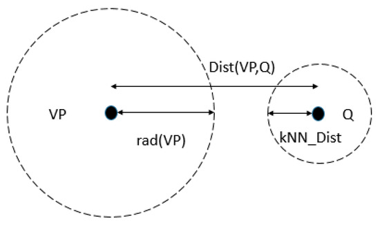
Figure 6.
Pruning the left subtree.
Second, if the following condition is satisfied, the right subtree is pruned.
In this case, the points of the VP’s right subtree are guaranteed to not be contained in the kNN of the query point, as shown in Figure 7. Otherwise, we should search the right subtree.
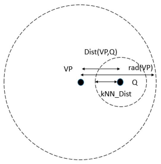
Figure 7.
Pruning the right subtree.
Therefore, we can reduce the kNN search time for the similarity hash using a VP tree. In Section 5, we will show the kNN search time using a VP tree.
4.3. Deep Learning–Based Malware Detection
The deep learning–based malware-detection method consists of two modules: feature extraction and deep learning. First, the feature-extraction module extracts the feature data from the portable executable (PE) files. Second, the deep-learning module trains a deep-learning model using training data and tests it using test data.
Figure 8 shows the complete deep learning–based malware-detection system.
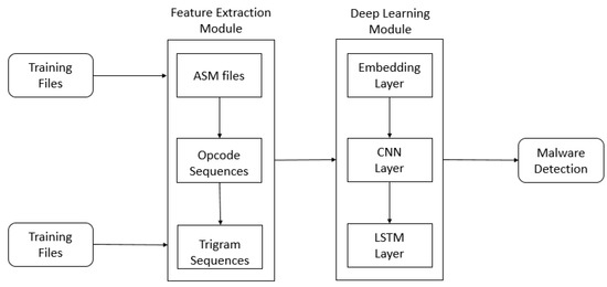
Figure 8.
Deep learning–based malware-detection system. ASM: assembler source language.
In the feature-extraction module, we convert the PE files into assembly-language (ASM) files using Objdump [13]. We extract opcode sequences from the ASM files and extract trigram sequences using three consecutive opcodes.
For example, Figure 9 shows an ASM file. Next, we extract an opcode sequence, as follows.
{add, inc, add, xchg, inc, add, movsb, inc}
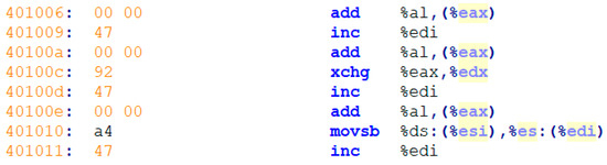
Figure 9.
ASM file.
Then, we construct trigram sequences using three consecutive opcodes, as follows.
{(add, inc, add), (inc, add, xchg), (add, xchg, inc), (xchg, inc, add), (inc, add, movsb),
(add, movsb, inc)}
In the deep-learning module, we train a deep-learning model that combines a CNN layer [15] and an LSTM layer [16] using training data, as shown in Figure 8. Then, we test it with test data. The CNN layer helps to obtain more features from the files and the LSTM layer helps to distinguish sequence data from other sequence data. In Section 5, we will show the detection rate of the deep-learning model.
5. Experimental Results
In Section 5.1, we introduce the experimental setup and, in Section 5.2, we give performance metric, and in Section 5.3, we provide the results.
5.1. Setup
We used 15,000 normal files and 15,000 malicious files, which were provided by the HAURI company [32]. We used five-fold cross validation [33]. First, we divided the files into five subsets; four subsets were used for training and one subset was used for testing. We repeated the experiments five times, replacing the test set each time. Thus, we used 12,000 normal files and 12,000 malicious files, which were randomly selected for training, and 3000 normal files and 3000 malicious files, which were randomly selected for testing.
We conducted two experiments. The first experiment compared the detection rate of the kNN classification with that of similarity hash–based detection, and compared the detection time of the kNN classification with that of the deep learning–based method. The second experiment compared the kNN search time using a VP tree with a brute-force search.
All experiments were performed on the Windows 10 operating system. The similarity hashes were computed using TLSH [11], and the VP tree [30] was implemented using JDK 12 [34]. The deep-learning model was implemented using Keras [35]. The detailed experimental conditions are described in Table 1.

Table 1.
Experimental environment.
5.2. Performance Metric
In this section, performance evaluation indicators are described, before presenting the experimental results. The indicators used in this study are accuracy, precision, recall (detection rate), F1 score, and false positive rate (FPR). The confusion matrix used to calculate these values is shown in Table 2.
Table 2.
Confusion Matrix.
TP indicates that a file has been correctly evaluated by the system to be malicious, and TN indicates that the system correctly determined that a benign file is normal. Furthermore, FP indicates that a normal file has been incorrectly judged by the system as malicious, and FN indicates that the system has incorrectly identified a malicious file to be normal. Each indicator is calculated as follows.
Accuracy = (TP + TN)/(TP + FP + FN + TN)
Precision = TP/(TP + FP)
Recall (Detection Rate) = TP/(TP + FN)
F1 score = 2 × Precision × Recall/(Precision + Recall)
FPR = FP/(FP + TN)
5.3. Results
In this section, we present the detection rates and the detection times of the kNN classification and provide the search time of a VP tree using a similarity hash.
5.3.1. NN Classification
We measured the detection rate and the detection time using 1NN classification. This detection rate was compared with the detection rate using only TLSH, and the detection time using 1NN classification was compared with the detection time using only the deep learning–based method.
Figure 10 and Table 3 show the detection rates of the 1NN classification and the deep learning together. We measured the detection rate when there were 24,000 training data, and 1500, 3000, 4500, and 6000 test data. The rate is compared with using only TLSH.
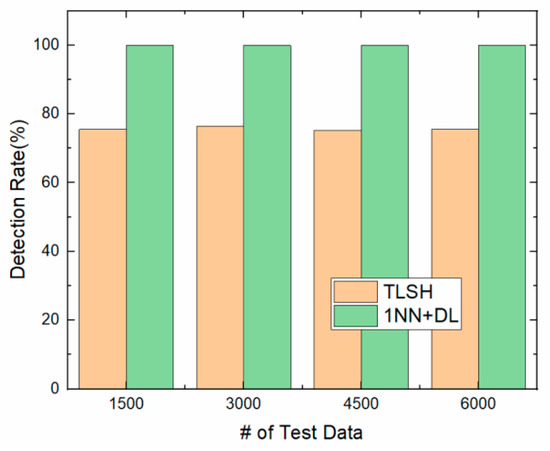
Figure 10.
Detection rates.
Table 3.
Experimental results.
The detection rate using only TLSH is about 75%. In the 1NN classification method, when a test file is assigned to the normal group or the malicious group, it is determined to be normal or malicious using only TLSH. However, if it is assigned to the undecided group, whether it is malicious or not is determined using the deep learning–based method. The detection rate of the 1NN classification and the deep learning together is 100%. Therefore, we increased the detection rate by 25% using the 1NN classification method.
Figure 11 shows the detection times of the 1NN and deep learning together. This is compared with only deep learning. We measured the detection time when there were 24,000 training data, and 1500, 3000, 4500, and 6000 test data. When there were 6000 test data, the detection time for the deep learning–based method was 171 s. In the 1NN classification method, when a test file is assigned to the normal group or the malicious group, it is determined to be normal or malicious, respectively, using only TLSH. Therefore, we can reduce the detection time. Meanwhile, when it is assigned to the undecided group, the deep learning–based method is used to determine whether or not it is malicious. The detection time of the 1NN classification and deep learning together was about 56 s for 6000 test data. Therefore, we reduced the detection time by 67% using the 1NN classification method.
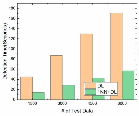
Figure 11.
Detection times.
5.3.2. VP Tree
In the second experiment, we measured the VP-tree generation time, number of distance comparisons, and the search time to find the 1NN. First, Figure 12 shows the VP-tree generation time. We measured the VP tree generation time when there were 6000, 12,000, 18,000, and 24,000 training data. When there were 24,000 training data, the VP-tree generation time was about 400 ms. We believe that it is reasonable.
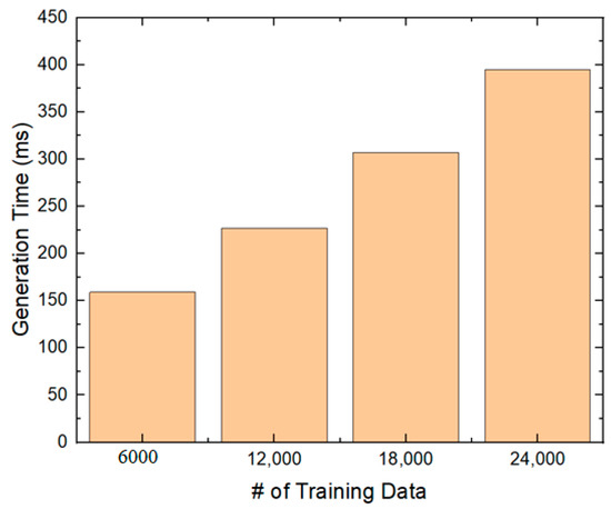
Figure 12.
VP-tree generation time.
Second, we measured the number of distance comparisons in the VP-tree search and compared it with the brute-force search. When we found the 1NN of the similarity hash, the distance comparison was the most important. When there were 24,000 training data, the number of distance comparisons in the brute-force search was 24,000, as shown in Figure 13. However, the number of distance comparisons in the VP-tree search was about 8902. By using the VP tree, we reduced the number of distance comparisons by about 60%.
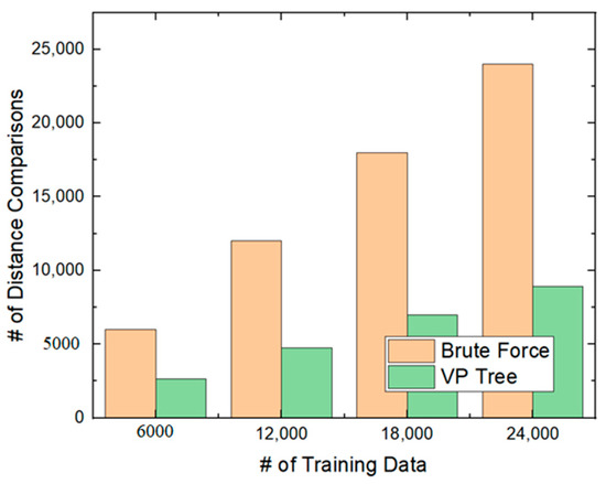
Figure 13.
Number of distance comparisons.
Third, we measured the 1NN search time of the VP tree when there were 6000 test data and compared it with the brute-force search. As shown in Figure 14, when there were 24,000 training data, the brute-force search time was about 13,300 ms, and the VP-tree search time was about 11,900 ms. By using the VP tree, we reduced the search time by about 20%, on average.
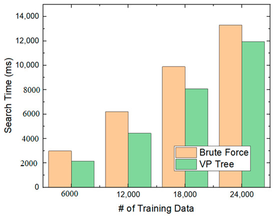
Figure 14.
Search times.
6. Discussion
In this paper, we proposed two methods to improve the speed of malware detection. First, we proposed a kNN classification to increase the detection rate and reduce the detection time. Second, we provided a similarity hash using a VP tree to improve the similarity-hash search speed. By using kNN classification, we increased the detection rate by 25% and decreased the detection time by 67%. By using the VP tree with a similarity hash, we reduced the search time by 20%.
In this study, we determined whether a file was malicious. Thus, we classified the files into a normal group, a malicious group, and an undecided group. However, there are different types of malware such as trojans, backdoors, worm, dropper, and viruses. Therefore, we need the kNN classification for specifying the type of malware. We can use the kNN classification two times. On the first use of the kNN classification, we classify files into a normal group, a malicious group, and an undecided group. On using the kNN classification the second time, we can classify malicious files into a trojan group, a backdoor group, a worm group, a dropper group, a virus group, and an undecided group.
Moreover, we propose a method for improving the VP tree to reduce search time. Originally, we expected that when there are n training files, the search time would be O(logn). However, we discovered that the query circle is often overlapped with the inner space and the outer space of the vantage point in the experiment. Thus, we had to search the left subtree and right subtree of the vantage point frequently. We expect that by using an m-tree [36] having m subtrees instead of a VP tree having two subtrees, we may reduce the search time.
On the other hand, there are recent researches about evading malware detection using GAN [22,23,24,25]. GAN can be used to modify malware using a generator to be determined as normal by a discriminator. It is reported that GAN significantly reduces the detection rate. We need a method to prevent evading malware detection. We expect that we may solve this problem to some extent using deep learning–and similarity hash–based detection methods together.
Funding
This work was supported by National Research Foundation of Korea (NRF) grant funded by the Korean government (MSIT) (No.2019R1G1A11100261) and the HPC support project supported by MSIT and NIPA.
Conflicts of Interest
The author declares no conflict of interest.
References
- AV-TEST. Available online: https://www.av-test.org (accessed on 15 June 2020).
- Gavriluţ, D.; Cimpoe¸su, M.; Anton, D.; Ciortuz, L. Malware Detection using Machine Learning. In Proceedings of the Internation Multiconference on Computer Science and Information Technology, Mragowo, Poland, 12–14 October 2009. [Google Scholar]
- Saxe, J.; Berlin, K. Deep Neural Network based Malware Detection using Two Dimensional Binary Program Features. In Proceedings of the International Conference on Malicious and Unwanted Software (MALWARE), Fajardo, Puerto Rico, 20–22 October 2015. [Google Scholar]
- Gibert, D. Convolutional Neural Networks for Malware Classification. Master’s Thesis, Universitat de Barcelona, Barcelona, Spain, 2016. [Google Scholar]
- Dahl, G.E.; Stokes, J.W.; Deng, L.; Yu, D. Large-scale Malware Classification using Random Projections and Neural Networks. In Proceedings of the International Conference on Acoustics, Speech and Signal Processing(ICASSP), Vancouver, BC, Canada, 26–31 May 2013. [Google Scholar]
- Pascanu, R.; Stokes, J.W.; Sanossian, H.; Marinescu, M.; Thomas, A. Malware classification with recurrent networks. In Proceedings of the International Conference on Acoustics, Speech and Signal Processing (ICASSP), Brisbane, Australia, 19–24 April 2015. [Google Scholar]
- Huang, W.; Stokes, J.W. MtNet: A Multi-task Neural Networks for Dynamic Malware Classification. In Proceedings of the International Conference on Detection of Intrusions and Malware and Vulnerability Assessment (DIMVA), San Sebastian, Spain, 7–8 July 2016. [Google Scholar]
- Ki, Y.; Kim, E.; Kim, H.K. A Novel Approach to Detect Malware Based on API Call Sequence Analysis. Int. J. Distrib. Sens. Netw. 2015, 11, 659101. [Google Scholar] [CrossRef]
- Bae, J.; Lee, C.; Choi, S.; Kim, J. Malware Detection Model with Skip-Connected LSTM RNN. J. Korean Inst. Inf. Sci. Eng. 2018, 45, 1233–1239. [Google Scholar] [CrossRef]
- Choi, S.; Bae, J.; Lee, C.; Kim, Y.; Kim, J. Attention-Based Automated Feature Extraction for Malware Analysis. Sensors 2020, 20, 2893. [Google Scholar] [CrossRef] [PubMed]
- Oliver, J.; Cheng, C.; Chen, Y. TLSH–A Locality Sensitive Hash. In Proceedings of the 4th Cybercrime and Trustworthy Computing Workshop, Sydney, Australia, 21–22 November 2013. [Google Scholar]
- Li, Y.; Sundaramurthy, S.C.; Bardas, A.G.; Ou, X.; Caragea, D.; Hu, X.; Jang, J. Experimental study of fuzzy hashing in malware clustering analysis. In Proceedings of the 8th USENIX Conference on Cyber Security Experimentaion and Test, Austin, PA, USA, 8 August 2015. [Google Scholar]
- Kendall, K.; McMillan, C. Practical Malware Analysis; BlackHat: Las Vegas, NV, USA, 2007. [Google Scholar]
- Moser, A.; Kruegel, C.; Kirda, E. Limits of Static Analysis for Malware Detection. In Proceedings of the 23rd IEEE International Conference on Computer Security and Applications, Miami Beach, FL, USA, 10–14 December 2007; pp. 421–430. [Google Scholar]
- Krizhevsky, A.; Sutskever, I.; Hinton, G. ImageNet Classification with Deep Convolutional Neural Networks. In Proceedings of the International Conference on Neural Information Processing Systems, Lake Tahoe, CA, USA, 3–6 December 2012. [Google Scholar]
- Understanding LSTM Netwoks. Available online: https://colah.github.io/posts/2015-08-Understanding-LSTMs/ (accessed on 27 July 2020).
- Srndic, N.; Lakov, P. Hidost: A Static Machine-Learning-based Detector of Malicious Files. EURASIP J. Inf. Secur. 2016, 2016, 22. [Google Scholar] [CrossRef]
- Hendler, D.; Kels, S.; Rubin, A. Detecting Malicious Powershell Commands using Deep Neural Networks. In Proceedings of the ACM ASIACCS, Songdo, Korea, 4–8 June 2018. [Google Scholar]
- Rusak, G.; Al-Dujaili, A.; O’Reilly, U. POSTER: AST-Based Deep Learning for Detecting Malicious Powershell. In Proceedings of the ACM CCS, Toronto, ON, Canada, 15–19 October 2018. [Google Scholar]
- Snell, J.; Swersky, K.; Zemel, R. Prototypical Networks for Few-shot Learning. In Proceedings of the 31st Conference on Neural Information Processing Systems, Long Beach, CA, USA, 4–9 December 2017. [Google Scholar]
- Tang, Z.; Wang, P.; Wang, J. ConvProtoNet: Deep Prototype Induction towards Better Class Representation for Few-Shot Malware Classification. Appl. Sci. 2020, 10, 2847. [Google Scholar] [CrossRef]
- Papernot, N.; McDaniel, P.; Goodfellow, I.; Jha, S.; Celik, Z.B.; Swami, A. Practical Black-Box Attacks against Machine Learning. In Proceedings of the ACM ASIACCS, Abu Dhabi, UAE, 2–6 April 2017. [Google Scholar]
- Hu, W.; Tan, Y. Generating Adversarial Malware Examples for Black-Box Attacks Based on GAN. arXiv 2017, arXiv:1702.05983. [Google Scholar]
- Hu, W.; Tan, Y. Black-Box Attacks against RNN Based Malware Detection Algorithms. In Proceedings of the Workshops of the Thirty-Second AAAI Conference on Artificial Intelligence, New Orleans, Lousiana, 2–7 February 2018. [Google Scholar]
- Rosenberg, I.; Shabtai, A.; Rokach, L.; Elovici, Y. Generic Black-box End-to-End Attack Against State of the Art API Call Based Malware Classifiers. In Proceedings of the International Symposium on Research in Attacks, Intrusions, and Defenses (RAID), Crete, Greece, 10–12 September 2018. [Google Scholar]
- Ieracitano, C.; Adeel, A.; Morabito, F.C.; Hussain, A. A novel statistical analysis and autoencoder driven intelligent intrusion detection approach. Neurocomputing 2019, 387, 51–62. [Google Scholar] [CrossRef]
- Gonzalez-Cuautle, D.; Hernandez-Suarez, A.; Sanchez-Perez, G.; Toscano-Medina, L.K.; Portillo-Portillo, J.; Olivares-Mercado, J.; Perez-Meana, H.M.; Sandoval-Orozco, A.L. Synthetic Minority Oversampling Techniques for Optimizing Classification Tasks in Botnet and Intrusion-Detection-System Datasets. Appl. Sci. 2020, 10, 794. [Google Scholar] [CrossRef]
- Lin, Z.; Shi, Y.; Xue, Z. IDSGAN: Generative Adversarial Networks for Attack Generation against Intrusion Detection. arXiv 2018, arXiv:1809.02077. [Google Scholar]
- Pearson, P.K. Fast Hasing of Variable-Length Text Strings. Commun. ACM 1990, 33, 677–680. [Google Scholar] [CrossRef]
- Yianilos, P.N. Data structures and algorithms for nearest neighbor search in general metric spaces. In Proceedings of the Fourth Annual ACM-SIAM Symposium on Discrete Algorithms, Austin, PA, USA, 25–27 January 1993. [Google Scholar]
- Khamsi, M.A.; Kirk, W.A. An Introduction to Metric Spaces and Fixed Point Theory; Wiley-IEEE: Hoboken, NJ, USA, 2001. [Google Scholar]
- HAURI, Antivirus Company. Available online: http://www.hauri.net (accessed on 15 June 2020).
- Cross Validation. Available online: https://machinelearningmastery.com/k-fold-cross-validation (accessed on 15 June 2020).
- JDK 12. Available online: https://oracle.com/javaj/technologies/javase-downloads.html (accessed on 15 June 2020).
- Keras. Available online: https://keras.io (accessed on 15 June 2020).
- Ciaccia, P.; Patella, M.; Zezula, P. M-tree An Efficient Access Method for Similarity Search in Metric Spaces. In Proceedings of the 23rd VLDB Conference, Athens, Greece, 25–29 August 1997. [Google Scholar]
© 2020 by the author. Licensee MDPI, Basel, Switzerland. This article is an open access article distributed under the terms and conditions of the Creative Commons Attribution (CC BY) license (http://creativecommons.org/licenses/by/4.0/).