Bearing Health Monitoring Using Relief-F-Based Feature Relevance Analysis and HMM

Abstract

Nowadays, bearings installed in industrial electric motors are constituted as the primary mode of a failure affecting the global energy consumption. Since industries’ energy demand has a growing tendency, interest for efficient maintenance in electric motors is decisive. Vibration signals from bearings are employed commonly as a non-invasive approach to support fault diagnosis and severity evaluation of rotating machinery. However, vibration-based diagnosis poses a challenge concerning the signal properties, e.g., highly dynamic and non-stationary. Here, we introduce a knowledge-based tool to analyze multiple health conditions in bearings. Our approach includes a stochastic feature selection method, termed Stochastic Feature Selection (SFS), highlighting and interpreting relevant multi-domain attributes (time, frequency, and time–frequency) related to the bearing faults discriminability. In particular, a relief-F-based ranking and a Hidden Markov Model are trained under a windowing scheme to achieve our SFS. Obtained results in a public database demonstrate that our proposal is competitive compared to state-of-the-art algorithms concerning both the number of features selected and the classification accuracy.

1. Introduction

Due to the sector competitiveness, high demand for fuel, and increasing power consumption, the industry interests are mainly related to cost-efficient operations. Namely, American manufacturers spent around USD 600 bi-million in the maintenance of critical systems in the early 1980s, and such expenses doubled within just 20 years [1]. Concerning this, electric motors consume nearly the 70% of energy, and major industries related to oil, petrochemical, and gas, determined that motor bearings account for 51% of failure modes [2]. Hence, machinery fault diagnosis related to bearings appears as a strategy to mitigate current industry challenges, which favors the detection of abnormal states in their early stages and prevents the appearance of more severe failures [3].

Regarding this, machinery fault diagnosis can be carried out through model-based, signal-based, or knowledge-based approaches. Model-based techniques detect changes in the machine behavior using a mathematical model of the system [4]; nonetheless, their success depends upon deterministic models of the industrial processes holding assumptions that can not correspond to the real management. Signal-based algorithms utilize measured data rather than specific input–output models for fault diagnosis [5]. Although a signal-based method provides a more realistic way to assess the fault than model-based ones, it depends on a symptom analysis from normal states, which is accomplished mainly by a field expert. Furthermore, finding a subset of useful sensors to record the signals is essential [6]. In turn, knowledge-based approaches deal with the diagnosis problem from a pattern recognition perspective, comprising: (i) a signal acquisition stage, (ii) a feature estimation procedure, and (iii) a fault assessment through learning algorithms [7]. In this context, the acquisition system should be both a non-invasive and non-destructive technique for extracting relevant information [8]. Recently, data acquisition systems-based on acoustic signals have gained demand over other non-contact measurement techniques. In particular, when the sensor locations on the machine are unavailable, or the measurement procedure has a risk for workers [9]. Notwithstanding, acoustic signals are more vulnerable to environmental noise than vibration responses [10]. Therefore, vibration signals are the most widely used method for machinery fault diagnosis, especially, from bearing [11].

Vibration signals from bearings are assumed to be quasi-stationary or non-stationary, with different fault diagnosis patterns even when data come from the same equipment [12]. Then, the signal characterization poses a challenge to code discriminative models. Commonly, feature estimation from vibration data comprises time, frequency, and time–frequency-based parameters [13,14]. Approaches devoted to time domain-based features focus on statistical measures. Still, they do not adequately reflect the change in frequency components as the progression of a fault develops [15]. Frequency-based features include the fast Fourier transform (FFT) and the power spectrum analysis. Authors in [16] introduced a power spectral density-based method to rotor fault detection from vibration signals. The technique can eliminate the influence of adverse disturbances on a diagnostic model of the machine. Likewise, authors in [17] propose a bearing health index based on the moving average cross-correlation of the power spectral density, which can track the health condition. Nevertheless, given the nature of the signals, such techniques are not suitable for identifying non-stationary events. Time-frequency features based on wavelet transform (WT) have obtained promising results in bearings fault diagnosis tasks [18]. Despite the advantage of the WT to deal with non-stationary patterns, only signal features that match with the wavelet shape can be detected [19]. Nonlinear dynamic methods emerged as alternatives to the process of feature estimation in machinery fault diagnosis, such as permutation entropy (PE) [20], multiscale entropy (MSE) [21], and multiscale permutation entropy (MPE) [22]. PE measures the randomness of the time series [23]; however, it analyzes the signal using one scale; so, fault information contained in other ranges is not coded. MSE uses a coarse-grained procedure to obtain a multiple-scale time series [24]. In MPE analysis, the entropy of the coarse-grained time series at each scale is calculated by the neighborhood preserving embedding algorithm. Still, MPE can not reveal relevant fault information because of its averaging algorithm. In contrast, authors in [25] proposes a generalized composite multiscale permutation entropy (GCMPE). Cheng He et al. [26] introduce a fault diagnosis method by combining extreme-point symmetric mode decomposition and composite multiscale weighted permutation entropy. Though entropy-based features can obtain reliable discrimination performances, the parameters estimated lack of suitable interpretability concerning the bearing fault diagnosis.

For the learning stage applied to the fault assessment, knowledge-based frameworks have been carried out by different unsupervised and supervised strategies, such as support vector machines [27]; metaheuristic-based algorithms [28]; Bayesian algorithms [29,30]; hidden Markov models (HMM) [31]; and deep learning [32,33]. Notably, authors in [34] introduce a method for diagnosing bearing faults based on deep learning and convolutional neural network layers. They use the raw vibration signals as input data, and the approach does not require any feature estimation. Moreover, authors in [35] propose a capsule network for fault diagnosis, which achieves high diagnostic accuracy in different working conditions. Shen et al. [36] proposed a hierarchical adaptive deep belief network, holding as inputs the frequency domain information and achieving high performance in the diagnosis of bearing fault types and damage levels. Further, authors in [37,38] proposed unsupervised diagnosis models based on frequency-domain features and deep learning. Yet, interpreting the relevance of the learned features through deep learning is not clear, and the overfitting is latent. HMM is a practical stochastic approach to code time-series dependencies that have been demonstrated promising vibration-based bearing fault diagnosis results [39]. In particular, as a dual random process, HMM has two main parameters, hidden states, and observation vector, which allow revealing the signal patterns from a stochastic perspective. Nevertheless, the learning stage often consists of a vast number of features, e.g., time, frequency, and time-frequency measures, meanwhile, the number of samples is limited due to the workload of data acquisition [40].

Hence, feature embedding and selection techniques are often used for dimensionality reduction to enhance the classification performance. The principal aim of this kind of methods is to reduce the number of features while increasing the classification accuracy [41]. Some feature-embedding techniques have been explored, including principal component analysis (PCA), which is a dimension compression method based on the minimum mean square error [42], and kernel principal component analysis (KPCA); as a nonlinear PCA extension by the introduction of a kernel-based mapping [43]. The former lack suitable representation when dealing with nonlinear dependencies, and the latter computes a feature space that loses the original engineering meaning (data interpretability). Accordingly, other dimensionality reduction methods known as feature selection are recommended [44,45]. Several techniques have been studied to select relevant features, such as the Laplacian score (LS), which evaluates the importance of features calculating its power of locality preserving [25]; the distance evaluation technique (DET) that indicates the degree of variation between samples from each feature provided [46]; scatter matrices (SM), as a supervised extension of the well-known PCA approach [47]; and the self-weight (SW) algorithm that adaptively evaluates the contribution of each attribute without class labels [45]. Recently, a feature ranking and subset selection based on Euclidean distance was proposed, employing a one-vs-one regulation between classes and features [48]. In turn, to efficiently extract fault feature information and improve fault diagnosis accuracy, an improved multiscale dispersion entropy and max-relevance min-redundancy feature selection is proposed in [49]. Authors in [50] integrated dimension reduction step to improve the efficiency of bearing fault detection. Though different feature-embedding and selection approaches have been proposed in the state-of-the-art, the coding of non-stationary and interpretable patterns for vibration-based bearing fault diagnosis and severity evaluation remains as an open issue [51].

In this work, a stochastic feature selection approach based on HMM is introduced to reveal relevant multi-domain features from vibration signals in bearing fault diagnosis and severity evaluation tasks. Our knowledge-based framework calculates time, frequency, and time–frequency domain-based features. Afterward, each feature relevance’s ranking is computed under a windowing scheme through a supervised cost function. In this sense, our feature ranking employs a local dissimilarity criterion using the relief-F method aiming to reveal local relationships among samples under a stochastic perspective governed by the windowing strategy and the HMM classifier. Further, we built a learning curve by adding one-by-one the features ranked, to code non-stationary and interpretable patterns concerning multiple health conditions in bearings. The results obtained in a public database of bearing diagnosis and severity evaluation, prove that our strategy is competitive compared to state-of-the-art approaches regarding the classification accuracy and the number of selected features.

The rest of the paper is organized as follows: In Section 2, we describe the theoretical framework. Then, in Section 3 we describe the experimental set-up. After, the obtained results and discussions are presented inSection 4. Finally, we outline the main remarks in Section 5.

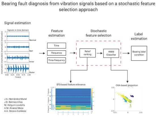
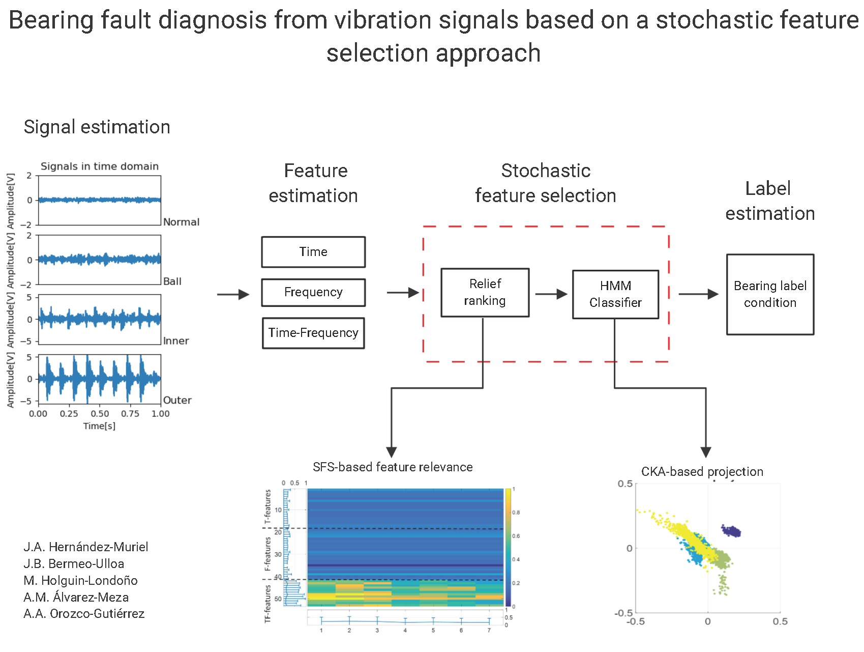
2. Stochastic Feature Selection

Let ${\{{\mathit{Z}}_n,y_n\}}_{n=1}^N$ be a set holding N vibration signals within a windowing approach. ${\mathit{Z}}_n\in {\mathbb{R}}^{W\times T}$ stores W row segments ${\mathit{z}}_{w,n}\in {\mathbb{R}}^T,$ at T time instants ($w\in \{1,2,\cdots ,W\}$), and $y_n\in \{1,2,\cdots ,C\}$ is the output label for the n-th signal concerning C fault diagnosis/severity classes of a bearing installed on a rotating machine. Here, we introduce a Stochastic Feature Selection (SFS) approach to support fault diagnosis/severity classification from vibration signals, which comprises the following main stages: (i) Multi-domain feature estimation and (ii) Supervised relevance analysis under stochastic modeling. The following describes in detail each stage.

2.1. Multi-Domain Feature Estimation

Since vibration signals hide complex and non-stationary dynamics, the following time, frequency, and time-frequency parameters are extracted from each segment $\mathit{z}\in \mathit{Z}$.

Time-based parameters (T): Time-domain features are computed as the natural representation of the input vibration signal [45,52]. So, we consider the statistical descriptors presented in

Table 1. Time domain features (T). Time-based parameters are computed for each vibration segment $\mathit{z}$.

Parameter	Estimation	Parameter	Estimation
Mean (${\mu }_{\mathit{z}}$)	$\sum _{t=1}^T{\displaystyle \frac{z_t}{T}}$	Skewness	$\sum _{t=1}^T{\displaystyle \frac{z_t^3}{T{{\rm Y}}_{\mathit{z}}^3}}$
Median	$\mathrm{median}\left(\mathit{z}\right)$	Max value	$\underset{t}{\max }\left(z_t\right)$
Standard deviation	${\left(\sum _{t=1}^T{\displaystyle \frac{{\left(z_t-{\mu }_z\right)}^2}{T}}\right)}^{1/2}$	Min value	$\underset{t}{\min }\left(z_t\right)$
Root mean square $\left({{\rm Y}}_{\mathit{z}}\right)$	${\left(\sum _{t=1}^T{\displaystyle \frac{z_t^2}{T}}\right)}^{1/2}$	Range	$|\underset{t}{\max }\left(z_t\right)-\underset{t}{\min }\left(z_t\right)|$
Peak (${\beta }_{\mathit{z}}$)	$\underset{t}{\max }\left(\right|z_t\left|\right)$	Interquartile range	$\mathrm{iqr}\left(\mathit{z}\right)$
Shape factor	${\displaystyle \frac{T{{\rm Y}}_{\mathit{z}}}{\sum _{t=1}^T\left|z_t\right|}}$	Kurtosis ($\kappa$)	$\sum _{t=1}^T{\displaystyle \frac{z_t^4}{T{{\rm Y}}_{\mathit{z}}^4}}$
Crest factor	${\displaystyle \frac{{\beta }_{\mathit{z}}}{{{\rm Y}}_{\mathit{z}}}}$	Speed kurtosis	$\kappa \left\{{\mathit{z}}^{\prime }\right\}$
Impulse factor	${\displaystyle \frac{T{\beta }_{\mathit{z}}}{\sum _{t=1}^T\left|z_t\right|}}$	Acceleration kurtosis	$\kappa \left\{{\mathit{z}}^{″}\right\}$
Clearance factor	${\displaystyle \frac{T^{1/2}{\beta }_{\mathit{z}}}{\sum _{t=1}^T{\left|z_t\right|}^{1/2}}}$	Acceleration kurtosis derivative	$\kappa \left\{{\mathit{z}}^{\prime ″}\right\}$

.

Frequency-based parameters (F): Frequency-based features are extracted based on the well-known fast Fourier transform (FFT) to code harmonic patterns [45,53]. Hence, a spectrum vector $\mathit{s}\in {\mathbb{C}}^K$ is computed as follows: $s_k=|{\sum }_{t=1}^T{z}_t{e}^{-i2\pi kt/T}|,$ where $z_t\in \mathit{z}$, $\mathit{\lambda }\in {\mathbb{R}}^K$ is a frequency index vector, ${\lambda }_k=kF/2K$, and $F\in \mathbb{R}$ is the sampling frequency $(k\in \{0,1,\cdots ,K\left\}\right)$. Then, we compute the statistical parameters shown in Table 1 and

Table 2. Frequency domain features (F). Frequency-based parameters are computed for each pair frequency and spectrum vectors $\mathit{\lambda }$, $\mathit{s}\in {\mathbb{R}}^K$.

Parameter	Estimation	Parameter	Estimation
Mean frequency (${\mu }_{\mathit{s}}$)	$\sum _{k=1}^K\frac{s_k}{K}$	Standard deviation frequency	${\left(\sum _{k=1}^K\frac{{({\lambda }_k-\Xi )}^2{s}_k}{K{\mu }_{\mathit{s}}}\right)}^{1/2}$
Central frequency ($\Xi$)	$\sum _{k=1}^K\frac{{\lambda }_k{s}_k}{K{\mu }_{\lambda }}$	Kurtosis	$\sum _{k=1}^K\frac{s_k^4}{K{\mu }_{\mathbf{s}}^2}$
Root mean square frequency	${\Xi }^{1/2}$

.

Time-frequency-based parameters (TF): Mel-frequency cepstral coefficients (MFCC) are used to highlight both linear and nonlinear patterns of the vibration signals [54,55]. Thus, from the FFT-based spectrum $\mathit{s},$ the log-energy output vector $\mathit{\vartheta }\in {\mathbb{R}}^R$ is computed towards a filter bank ${\{{\mathit{\eta }}_r\in {\mathbb{R}}^K\}}_{r=1}^R$ of size R in the Mel-scale, yielding: ${\vartheta }_r=log\left(\mathit{s}{\mathit{\eta }}_r^{\top }\right).$ Next, H MFCC are stored in the vector $\mathit{\iota }\in {\mathbb{R}}^H$, which is computed as the discrete cosine transform (DCT) of the logarithm Mel spectrum:

$${\iota }_h=\sum _{r=1}^R{\vartheta }_{r}cos\left(h\frac{\pi }{R}\left(r+\frac{1}{2}\right)\right).$$

(1)

Lastly, once all the aforementioned parameters are computed for all provided segments, a multi-domain feature set ${\{{\mathit{X}}_n,y_n\}}_{n=1}^N$ is built after concatenation of the T, F, and TF parameters of each ${\mathit{z}}_{w,n}$ in the row vector ${\mathit{x}}_{w,n}\in {\mathbb{R}}^M$ of ${\mathit{X}}_n\in {\mathbb{R}}^{W\times M},$ being M the number of multi-domain features extracted.

2.2. Supervised Relevance Analysis under Stochastic Modeling

In a practical application, the calculated multi-domain feature set ${\left\{{\mathit{X}}_n\right\}}_{n=1}^N$ has a vast number of parameters. This fact introduces noise and complexity for detecting/diagnosing tasks. Therefore, it is necessary to identify the most discriminating features to find a balance between system complexity and accuracy [44]. To achieve this aim, we compute the contribution of each T, F and TF parameters in terms of the supervised information in the labels vector $\mathit{y}={\left\{y_n\right\}}_{n=1}^N$. Our approach intends to codify the stochastic behavior in each feature matrix ${\mathit{X}}_n$ for the n-th vibration signal using a localized dissimilarity under supervised constraints and an HMM-based classifier. Initially, let $\mathsf{\Gamma }\in {\mathbb{R}}^{N\times Q}$ be a feature matrix holding row feature vectors $\mathit{\gamma }=\mathrm{vec}\left({\mathit{X}}_n\right),$ where $\mathrm{vec}\left(·\right)$ stands for the vectorization function. We calculate the relevance vector $\mathit{\nu }\in {\mathbb{R}}^Q$ using the relief-F-based gain [56]:

$${\mathrm{Gain}}_q=\frac{1}{N}\sum _{n=1}^N\left(-\frac{1}{\phi }\sum _{{\mathbf{\gamma }}_{n^{\prime }}\in {\Omega }_n^{y_n}}d({\gamma }_n^q,{\mathit{\gamma }}_{n^{\prime }}^q)+\frac{1}{\phi }\sum _{c\ne y_n}\frac{p(\mathit{y}=c)}{1-p(\mathit{y}=y_n)}\sum _{{\mathit{\gamma }}_{n^{\prime }}\in {\Omega }_n^{y_n}}d({\gamma }_n^q,{\gamma }_{n^{\prime }}^q)\right),$$

(2)

where $d:\mathbb{R}\times \mathbb{R}\to \mathbb{R}$ is a given distance function, ${\Omega }_n^c=\{{\mathit{\gamma }}_{n^{\prime }}:n^{\prime }=1,2,\cdots ,\phi \}$ holds the $\phi$-nearest neighbors of ${\mathit{\gamma }}_n$ according to d,${\gamma }_n^q\in \mathbb{R}$ is the value of the q-th feature for instance n, and $p(\mathit{y}=c)\in {\mathbb{R}}^{+}$ is the probability that a sample belongs to the $c$-th class ($c\in \{1,2,\cdots ,C\}$); $q\in \{1,2,\cdots ,Q\}$. In this sense, the localized measure in Equation (2) allows quantifying the discrimination capability of the T, F, and TF parameters. In fact, the higher the ${\nu }_q$ value, the better the q-th feature for discriminating fault categories in bearing diagnosis [57]. Now, to estimate the relevance of the M multi-domain features under the windowing scheme, we sort the vector $\mathit{\nu }$ into a feature relevance matrix $\mathsf{\Delta }\in {\mathbb{R}}^{W\times M}$ concerning the W segment partitions, as follows:

$$\mathsf{\Delta }=\left[\begin{array}{cccc}{\nu }_1& {\nu }_2& \cdots & {\nu }_M\\ {\nu }_{M+1}& {\nu }_{M+2}& \cdots & {\nu }_{2M}\\ ⋮& ⋮& \ddots & ⋮\\ {\nu }_{W(M-1)+1}& {\nu }_{W(M-1)+2}& \cdots & {\nu }_{WM}\end{array}\right].$$

(3)

In turn, the M multi-domain features can be ranked according to the value of the relevance vector $\mathit{\rho }\in {\mathbb{R}}^M$, holding elements:

$${\rho }_m=\frac{1}{W}\sum _{w=1}^W|{\Delta }_{wm}|,$$

(4)

where ${\Delta }_{wm}\in \mathsf{\Delta }$ and $m\in \{1,2,\cdots ,M\}$. As a result, our feature ranking allows explaining the measured locality preservation capability provided by each feature along with the W segments of the input vibration signals, since the obtained relevance vector $\mathit{\rho }$ preserves the one-to-one relationship to the multi-domain parameters.

Further, a Hidden Markov Model (HMM) was employed to represent the stochastic behavior of the W segments in ${\mathit{X}}_n$. Indeed, the use of hidden states makes the classification model generic enough to handle a variety of bearing fault diagnosis/severity classes [31,58,59]. Then, given an observation sequence matrix $\tilde{\mathit{X}}\in {\mathbb{R}}^{W\times M^{\prime }}$ which was built after the selection of the $M^{\prime }<M$ most relevant features according to the locality preservation capability in $\mathit{\rho }$, that is, $\tilde{\mathit{X}}$ holds the $M^{\prime }$ features that exhibit the highest ${\rho }_m$ values, a HMM can be defined by the set of parameters $\Psi =\{\mathbf{\Pi },\mathit{b},{\mathit{p}}_o\}$ and the set of states $\mathcal{S}={\{{\mathit{\theta }}_v\in {\mathbb{R}}^{M^{\prime }}\}}_{v=1}^V$. The matrix $\mathbf{\Pi }{[0,1]}^{V\times V}$ holds the state transition probabilities with ${\Pi }_{v{v}^{\prime }}=P\left({\theta }_{j+1}=v^{\prime }|{\theta }_j=v\right);$ ($v,v^{\prime },j=\{1,2,\cdots ,V\}$, $P(·|·)$ is a conditional probability distribution), and $\mathit{B}={\left\{b_v(·)\right\}}_{v=1}^V$ is an output probability function set, defined as follows:

$$b_v\left({\tilde{\mathit{x}}}_w\right)=\sum _{u=1}^U{\varpi }_{vu}\mathcal{N}\left({\tilde{\mathit{x}}}_w\right|{\mathit{\vartheta }}_{vu},{\mathbf{\Sigma }}_{vu}),$$

(5)

where ${\tilde{\mathit{x}}}_w\in {\mathbb{R}}^{M^{\prime }}$ is the w-th observation in $\tilde{\mathit{X}}$, U is the number of mixtures used to model the overall probability distribution, ${\varpi }_{vu}\in [0,1]$ is a mixture weight, ${\mathit{\vartheta }}_{vu}\in {\mathbb{R}}^{M^{\prime }}$ and ${\mathbf{\Sigma }}_{vu}\in {\mathbb{R}}^{M^{\prime }\times M^{\prime }}$ are the mean vector and the covariance matrix for the state v and the mixture u, respectively, and $\mathcal{N}(·)$ denotes a normal distribution. Moreover, ${\mathit{p}}_o\in {\mathbb{R}}^V$ is the vector of initial state probabilities.

Successively, a classifier can be trained from each bearing fault class, thereby, a model set $\Lambda =\{{\widehat{\mathbf{\Psi }}}_c:c\in \{1,\cdots ,C\}\}$ is computed as the following maximum likelihood estimation:

$${\widehat{\mathbf{\Psi }}}_c=arg\underset{\Psi }{max}P\left({\tilde{\mathit{X}}}_n\right|\mathbf{\Psi });\forall \{\widetilde{{\mathit{X}}_n}:y_n=c\}.$$

(6)

Finally, given a new matrix of feature segments ${\tilde{\mathit{X}}}_{*}\in {\mathbb{R}}^{W\times M^{\prime }}$, a HHM-based classification rule is given by:

$${\widehat{c}}_{*}=arg\underset{c}{max}P\left({\tilde{\mathit{X}}}_{*}\right|{\mathbf{\Psi }}_c).$$

(7)

In practice, the optimization problem in Equation (6) can be solved using an Expectation- Maximization-based approach [60].

Figure 1 summarizes the pipeline of the proposed bearing fault diagnosis system based on our SFS approach. Note that the time complexity of our SFS resides in the Relief-F and HMM required number of operations. Thereby, Relief-F boats a time complexity of $\mathcal{O}(N\times Q)$ meanwhile the HMM requires $\mathcal{O}(N^2\times Q)$ [61,62]. Our SFS’s MatLab implementation can be found at a GitHub repository (https://github.com/SiegE89/KBS-2018).

3. Experimental Setup

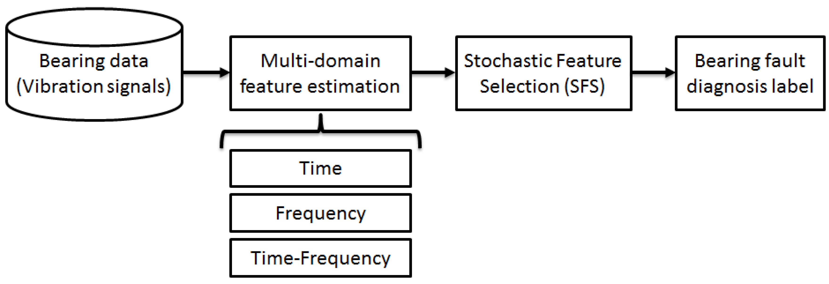
3.1. Database and Preprocessing

To test the proposed SFS approach, a publicly available bearing data collected by the Case Western Reserve University (K.A. Loparo, Bearing data center. Case Western Reserve University (2003)) (CWRU) is utilized in this paper. The experimental setup mainly included a three-phase induction motor, a torque transducer/encoder, a dynamometer, and electronic control. SKF bearings under different states were attached to the motor shaft. Two accelerometers were attached to the housing with magnetic bases in both drive and fan end. The faults ranged in diameter and were seeded on the drive- and fan-end bearings (SKF deep groove ball bearings: 6205-2RS JEM and 6203-2RS JEM, respectively) of the motor using electro-discharge machining. The faults were seeded on the rolling elements and the inner and outer races, and each faulty bearing was reinstalled (separately) on the test rig. Further, it was run at a constant speed for motor loads of 0 to 3 horse-power. The database was acquired from the experimental test bench under the following bearing states: Normal, a fault in the inner race, a fault in the outer race, and a fault in rolling element (electro-discharge machining artificially produced fault states). Additionally, the failure states were produced with three levels of severity (0.007″, 0.014″, and 0.021″) and three operation revolutions (1730, 1750, and 1797 [rpm]). As a consequence, 56 signals of 10 seconds (approximately) were acquired [63]. Although the CWRU provides vibration signals collected with a 16 channel DAT recorder using two different sample rate values (12 kHz and 48 kHz), we only considered the signals acquired with $F_s=48$ kHz to cover the whole harmonic patterns of the bearing states following the recommendations in [64].

Each vibration signal was pre-segmented using a rectangular window of 85.33 ms length (without overlapping); This value was selected following the Nayana et al. methodology in [65]. Therefore, an input matrix holding $N=5610$ samples is calculated. Two different diagnosis/detection scenarios were considered for bearing condition monitoring by varying the label vector: (i) four-class problem (C = 4), learning only the bearing state; and (ii) ten-class problem (C = 10), which includes state diagnosis and fault severity detection, as shown in

Table 3. Description of the different diagnosis/detection scenarios considered for bearing condition monitoring.

C = 4 Problem		C = 10 Problem
Id	Bearing State	Id	Bearing State	Fault Diameter	Id	Bearing State	Fault Diameter
N	Normal	N	Normal	-	IR2	Fault in inner race	0.014″
B	Fault in rolling element	B1	Fault in rolling element	0.007″	IR3	Fault in inner race	0.021″
IR	Fault in inner race	B2	Fault in rolling element	0.014″	OR1	Fault in outer race	0.007″
OR	Fault in outer race	B3	Fault in rolling element	0.021″	OR2	Fault in outer race	0.014″
		IR1	Fault in inner race	0.007″	OR3	Fault in outer race	0.021″

. To adjust the data set according to the methodology proposed, each signal is segmented using a Hamming window of 21.33 ms size and 50% overlapping. These values were chosen according to the approach presented by authors in [54,66]. As a consequence, $W=7$ windows of analysis are studied.

3.2. SFS Training

For concrete testing, our SFS approach includes 56 multi-domain features: 18, 23, and 12 for time, frequency, and time-frequency domains, respectively. To favor reliable estimations regarding the frequency-based features, the spectrum vector size is set at $K=4096$ to compute the parameters showed in Table 1 and Table 2. To calculate the TF parameters, we utilized a filter bank with $R=3·\log \left(F_s\right)=32$ Mel-filters applied over each spectrum holding $K=512$ values in frequency domain. In turn, we constructed the multi-domain feature set ${\{{\mathit{X}}_n\in {\mathbb{R}}^{W\times M}\}}_{n=1}^N$ holding $N=5610$ samples with $W=7$ windows and $M=53$ features. Later, a vector concatenation was applied over ${\mathit{X}}_n$ to yield a vector $\mathbf{\Gamma }\in {\mathbb{R}}^Q$, with $Q=W\times M=371$. In this sense, two parameters were selected to compute the relevance vector, in concordance with Equation (2): $\phi =1$ and $d({\gamma }_n^q,{\gamma }_{n^{\prime }}^q)=|{\gamma }_n^q-{\gamma }_{n^{\prime }}^q|/({max}_n\left({\gamma }_n^q\right)-{min}_n\left({\gamma }_n^q\right))$ [51,57]. Then, we constructed the feature relevant matrix $\mathit{\Delta }$ using Equation (3), and next, we estimated the relevance vector $\mathit{\rho }$ as shown in Equation (4). Due to the high number of samples, we consider a representative subset of data by using a clustering approach based on the well-known k-means algorithm [67]. In particular, $N_{c4}=3413$ and $N_{c10}=4141$ samples are preserved for the $C=4$ and $C=10$ classes, respectively. Besides, an HMM-based classifier is trained to fix the number of states and Gaussian mixtures to $V=2$, according to [54], and $U=2$ (value empirically selected). Lastly, we calculated the classification accuracy over the testing set by using a nested 10-fold cross-validation scheme, by adding, one-by-one, the features ranked based on the relevance values in $\mathit{\rho }$ (learning curve).

3.3. Method Comparison

For comparison purposes, we considered the following representative unsupervised and supervised feature selection methods: (i) variance-based relevance analysis (VRA), as an unsupervised method that generates a feature ranking based on a variability criterion (PCA) [68]. (ii) Self-weight ranking (SW), as an unsupervised technique, coding the feature relevance in terms of a self-similarity measure [45]. (iii) Laplacian score (LS), as an unsupervised approach that computes a relevance ranking from input samples to highlight the importance of each provided characteristic from graph edges [25]. (iv) Distance weight (DW) as a supervised method quantifying the relevance of the distance between samples from different clusters [69]. It is worth noting that whole provided feature selection algorithms are employed to rank the multi-domain parameters to build an HMM classifier performance curve by adding them one-by-one under a nested 10-fold cross-validation strategy. Furthermore, the achieved discrimination accuracy of relevant state-of-the-art approaches devoted to the Case Western Reserve University database classification, are also included in Section 4 for comparison purposes.

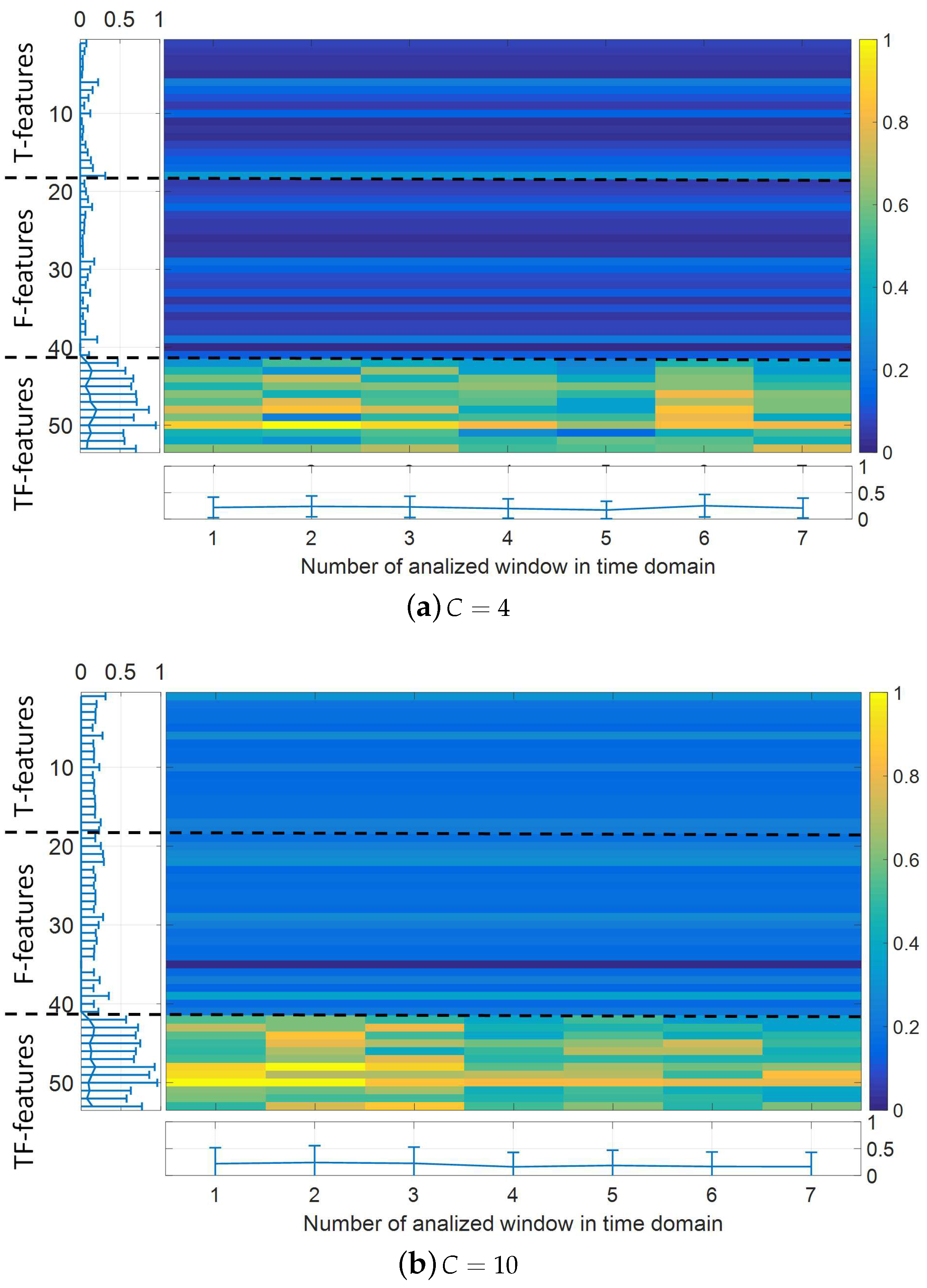
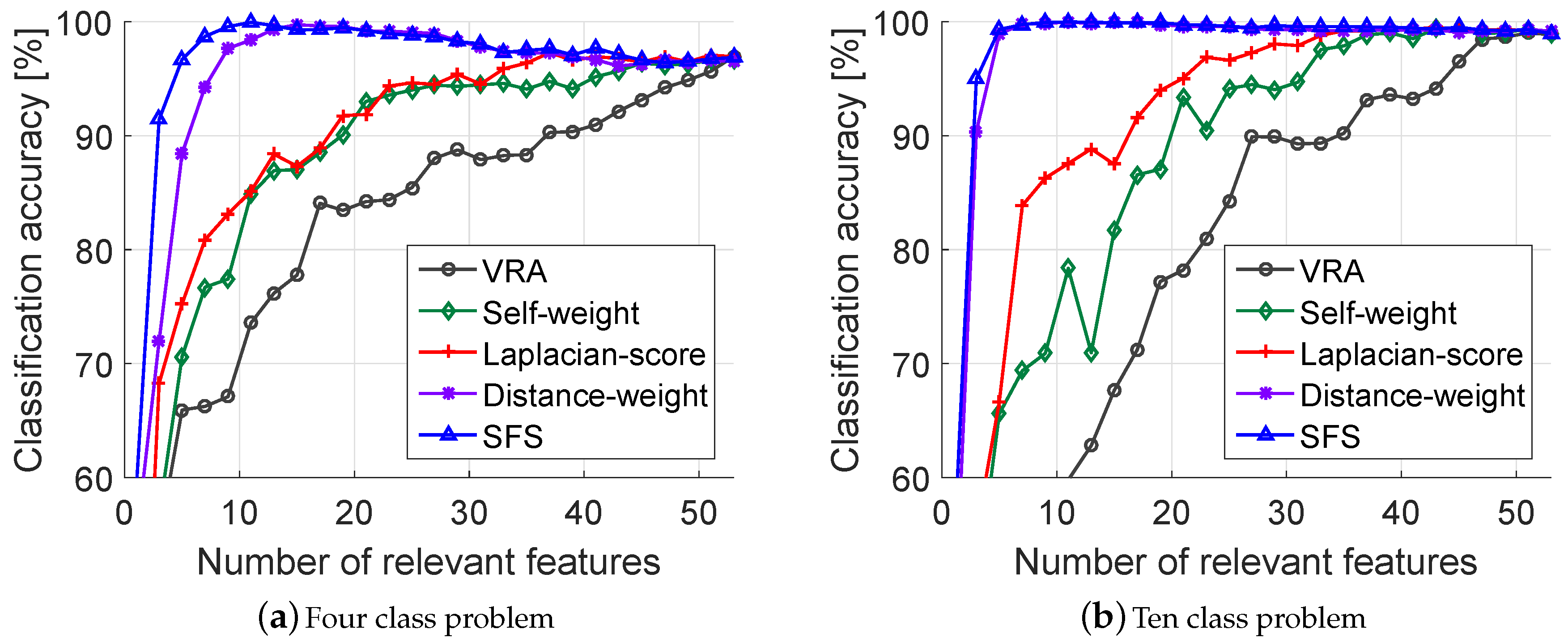
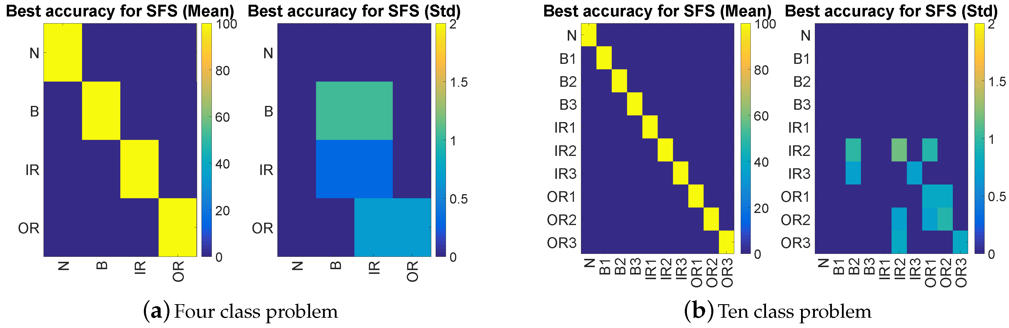
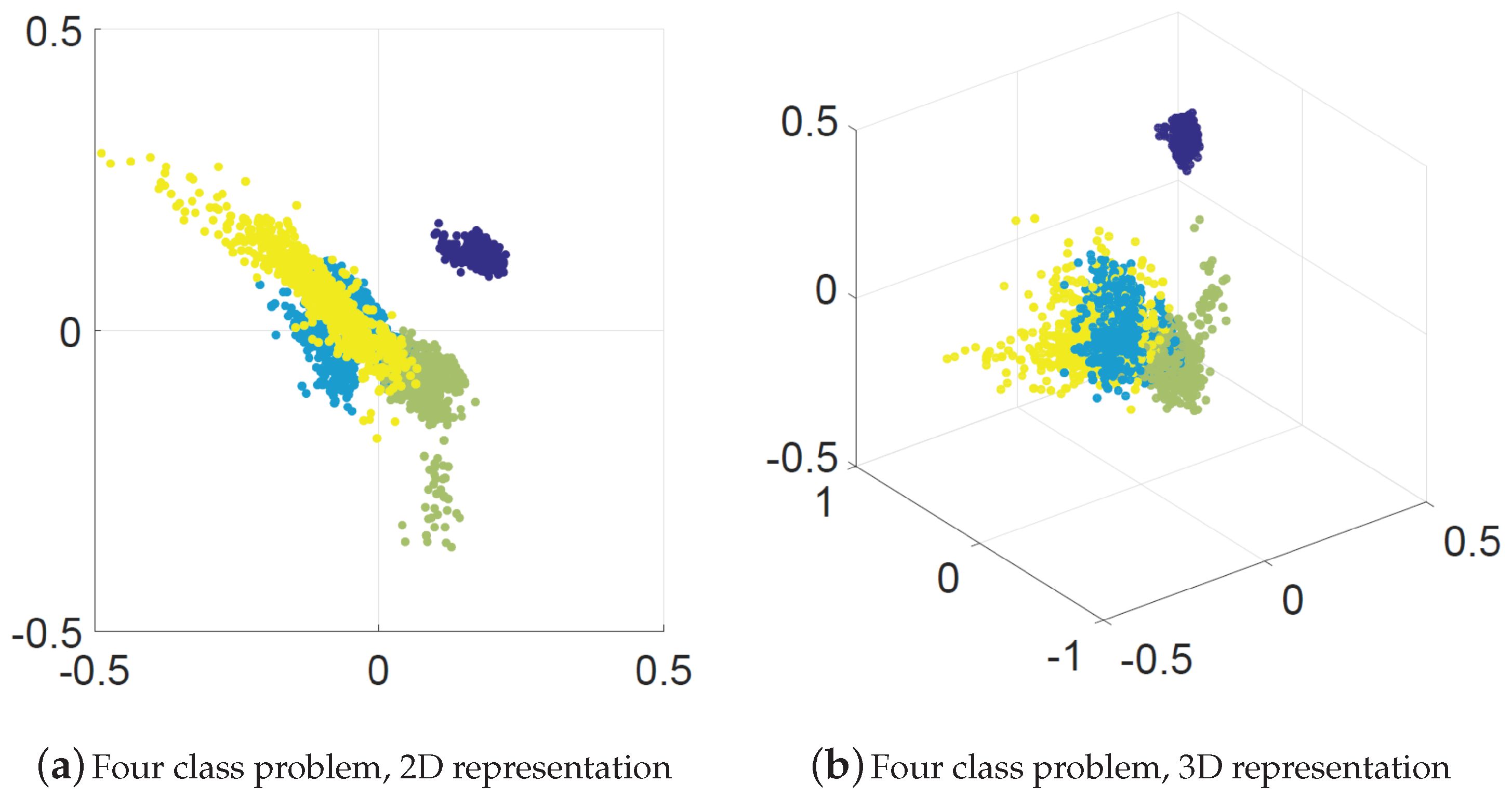
4. Results and Discussion

First, we introduce an illustrative example of the time and frequency parameters concerning the four classes problem. Figure 2 shows the time-domain waveform of some vibration segments with their corresponding frequency spectrum. As seen, the frequency spectrum varies for every bearing state. Besides, the main harmonic information is contained until 9 kHz. Now, Figure 3 shows the SFS-based feature relevance values for both $C=4$ and $C=10$ scenarios. Accordingly, the most relevant features are those calculated in the TF domain. Indeed, Mel-cepstrum measures exhibit the highest importance of the studied segments. Then, such parameters in TF can code both temporal and frequency information to support the identification of non-stationary bearing fault patterns.

The bearing fault diagnosis and evaluation results are exposed in Figure 4, which displays the learning curves obtained for the four and ten class problems. The VRA, SW, LS, DW, and the SFS-based rankings are studied using an HMM-based classification (see Section 3). Besides,

Table 4. Best classification results and number of features required (four class problem).

Method	# Feat.	Best Acc. (%)	Best # Feat.	Acc (%)
No feature selection	53	$96.97\pm 0.83$	-	-
VRA	53	$96.92\pm 0.84$	51	$95.63\pm 1.07$
Self-weight	53	$96.69\pm 0.76$	41	$95.17\pm 1.06$
Laplacian Score	37	$97.28\pm 0.92$	33	$95.87\pm 0.79$
Distance-weight	15	$99.74\pm 0.29$	13	$99.36\pm 0.39$
SFS	11	$99.94\pm 0.12$	9	$99.56\pm 0.40$

and

Table 5. Best classification results and number of features required (ten class problem).

Method	# Feat.	Best Acc. (%)	Best # Feat.	Acc (%)
No feature selection	53	$98.97\pm 0.46$	-	-
VRA	51	$99.01\pm 0.42$	47	$98.47\pm 0.58$
Self-weight	43	$99.39\pm 0.43$	37	$98.84\pm 0.62$
Laplacian Score	43	$99.53\pm 0.33$	33	$98.80\pm 0.49$
Distance-weight	11	$99.95\pm 0.07$	7	$99.76\pm 0.11$
SFS	11	$99.91\pm 0.16$	7	$99.74\pm 0.21$

show in the center column the best-achieved classification results and the number of features ranked by each method and in the right column the classification accuracy statistically equal to the best using fewer features. It is possible to note that the VRA method holds a classification accuracy of $\{95.63\pm 1.07\}\%$ for $C=4$ and $\{99.01\pm 0.42\}\%$ for $C=10$, but requiring 51 and 47 features, respectively. Moreover, achieved results demonstrate that unsupervised approaches, e.g., VRA, SW, and LS, cannot reveal relevant features in comparison to the supervised ones, e.g., DW and SFS. Though after 20 relevant features, the SW and LS algorithms attain an acceptable discrimination performance (a classification accuracy greater than $90\%$), the supervised methods accomplish such a classification threshold using less than ten features. Supervised approaches avoid the inclusion of redundant parameters as the performance curve falls after ten features, showing that the newly added features decrease the discrimination accuracy as they add unnecessary (noisy) information. In fact, the DW-based ranking exhibits classification accuracies of $\{99.36\pm 0.39\}\%$ ($C=4$) and $\{99.76\pm 0.11\}\%$ ($C=10$), using 13 and seven relevant features, respectively. Likewise, our SFS approach, which includes a relief-f-based feature selection, reaches $\{99.56\pm 0.040\}\%$ and $\{99.74\pm 0.21\}\%$ classification accuracies using nine features for $C=4$ problem and seven parameters for $C=10$. So, the SFS approach converges faster than the DW technique. In a nutshell, Table 4 and Table 5, present the best classification accuracies and the number of relevant features required for the $C=4$ and the $C=10$ problems, regarding the studied feature rankers. In turn, note that the supervised approaches’ time complexity highly depends on the number of samples (see Section 2.2 for SFS analysis). Nonetheless, the training is offline, and the number of selected features is much lower than the number of input attributes, alleviating the time complexity of the testing set prediction.

Figure 5 shows the confusion matrix obtained for both classification scenarios using only the relevant features computed by our SFS. As seen, the accuracy in both cases is closer to $100\%$. On the one hand, for the four-class problem, the B, IR, and OR classes tend to be slightly confused, while the N class is classified satisfactorily. On the other hand, for the ten class problem, the N, B1, B2, B3, and IR1 are correctly detected; however, data belonging to the IR2, IR3, OR1, OR2, and OR3 classes still tend to be slightly confused with other bearing states. It is worth noting to mention that the inclusion of a suitable feature selection approach increases the accuracy of the HMM-based classifier adopting a few numbers of relevant features (interpretable measures). At the same time, it helps to get a better representation space for visualizing the data distribution. In this sense, Figure 6 shows a 2D and 3D data projection based on the centered kernel alignment (CKA) algorithm applied to the relevant features computed by our SFS approach. CKA projects the original domain’s data into rotated points of lower dimensionality space, evaluating the similarity between an input kernel matrix (given by the relevant features set) and a target kernel computed over the output labels [70]. As seen, the separability between N and failure states are clear; additionally, the representation displays overlapping between samples belonging to the B, IR, and OR classes, as before corroborated by the confusion matrices and by other state-of-the-art approaches [71].

Table 6. A comparative study between current work and previous approaches published in the state-of-art for bearing fault diagnosis on the Western Case University Bearing database.

Reference	${\mathit{F}}_{\mathit{s}}$ (kHz)	Number of Classes	Labels	Feature Extraction	Feature Selection	Number of Features	Classifier	Accuracy (%)
William and Hoffman [72]	12	4	$IR,OR,B,N$	ZC	-	10	ANN	97.13
Muruganatham et al. [74]	12	4	$IR,OR,B,N$	SSA	-	10	ANN	96.53
Tiwari et al. [22]	48	4	$IR,OR,B,N$	MPE	-	16	ANFC	97.50
Zhang et al. [27]	12	4	$IR,OR,B,N$	PE+EEMD	-	12	SVM+ICD	97.75
Ocak and Loparo [77]	12	3	$IR,OR,B$	LPM	-	30	HMM	99.67
Yuwono et al. [59]	12	3	$IR,OR,B$	WT+CL	-	12	HMM+SRCE	95.08
Muruganatham et al. [74]	12	4	$IR,OR,B,N$	SSA	SV	4	ANN	95.14
Shen et al. [75]	12	4	$I{R}_1,O{R}_1,B,N$	WPT+SP	DET	30	SVR	100.00
Shen et al. [75]	12	4	$I{R}_2,O{R}_2,B,N$	WPT+SP	DET	30	SVR	100.00
Van et al. [46]	-	7	$I{R}_1,I{R}_2,O{R}_1,O{R}_2,B_1,B_2,N$	TD+SP, FD+SP, EMD+SP	DET+PSO-KNN	20	KNN	98.58
Van et al. [46]	-	7	$I{R}_1,I{R}_2,O{R}_1,O{R}_2,B_1,B_2,N$	TD+SP, FD+SP, EMD+SP	DET+PSO-KNN	5	PNN	97.24
Van et al. [46]	-	7	$I{R}_1,I{R}_2,O{R}_1,O{R}_2,B_1,B_2,N$	TD+SP, FD+SP, EMD+SP	DET+PSO-KNN	6	SVM	97.71
Brkovic et al. [47]	12	4	$IR,OR,B,N$	WT+SP	SM	12	QC	100.00
Liang et al. [44]	48	4	$IR,OR,B,N$	TD+SP, FD+SP	NMF+ALS+SCD	3	KNN	92.86
Zheng et al. [25]	12	6	$I{R}_1,I{R}_2,O{R}_1,O{R}_2,B,N$	GCMPE	LS	2	PSO-SVM	98.89
Jian et al. [71]	12	10	$I{R}_1,I{R}_2,I{R}_3,O{R}_1,O{R}_2,O{R}_3,B_1,B_2,B_3,N$	ACNN-W	-	10	ACNN-W	98.66
Toufik et al. [76]	12	6	$I{R}_1,I{R}_2,I{R}_3,O{R}_1,O{R}_2,B$	FES	IRO	11	MMV	96.08
SFS (our work)	48	4	$IR,OR,B,N$	TD+SP, FD+SP, TFD+SP	Relief-F	9	HMM	99.56
SFS (our work)	48	10	$I{R}_1,I{R}_2,I{R}_3,O{R}_1,O{R}_2,O{R}_3,B_1,B_2,B_3,N$	TD+SP, FD+SP, TFD+SP	Relief-F	7	HMM	99.74

presents a comparative study of the achieved SFS results and state-of-art approaches devoted to bearing fault diagnosis and its evaluation. Here, two main aspects are deemed: (i) the method has to be proven on the Western Case University database, and (ii) the metric used to evaluate the diagnosis/evaluation performance has to be the classification accuracy. It is possible to observe that the proposed SFS approach outperforms the majority of the studied methodologies concerning the trade-off between classification accuracy and the required number of features. Additionally, note that a significant amount of methods do not include a feature selection stage. Still, at the expense of lower classification accuracy [22,27,72,73,74]. On the other hand, methodologies that incorporate feature selection techniques demonstrate better discrimination results [44,46,47,74,75]. In particular, two proposals stand out: the work presented by Zheng et al. in [25] and our SFS-based approach. Although the first one uses the smallest number of features, the experimental results reported in the paper were calculated using a simple validation framework. They employed only 174 samples (24 per class) to generate two subsets of data (84 samples for training and 90 for testing). Besides, our methodology can identify both the bearing state and the severity level of all the fault listed in the database; meanwhile, the work presented in [25,76] only considers six classes. Note that the T, F, and TF-based parameters computed in SFS represent a significant advantage since the experts can interpret them. For example, they can analyze the evolution of the energy in a frequency band to identify a failure state. Remarkably, the work presented by authors in [71] also exhibits outstanding performances. They consider a ten class problem, in which different methodologies based on neural networks are used. However, neural network frameworks lack suitable feature relevance interpretability concerning the input space, not to mention their high computational cost.

5. Conclusions

In this work, we introduced a stochastic feature selection approach, called SFS, to support bearing fault diagnosis and severity evaluation from vibration signals. Our method comprises the following stages: (i) multi-domain feature estimation using time, frequency, and time–frequency parameters, and (ii) supervised relevance analysis under stochastic modeling that includes feature ranking based on a relief-f algorithm and HMM-based classification. So, our approach gathers a subset of multi-domain parameters under a windowing scheme to favor HMM discrimination. We test our SFS over a public bearing fault database under different conditions. According to the obtained results, the time–frequency-based features are the most relevant for separating the type of fault and severity levels. Achieved classification results demonstrated that our proposal is competitive and even exceeded the state-of-the-art works concerning both discrimination accuracy and the number of required features. Our strategy extracts a relevant subset of features that favors further learning stages by coding complex data relationships related to hidden interactions between fault type and severity levels. Besides, the statistical parameters computed by the SFS approach represent a significant advantage since experts can interpret them in the field. As future work, the authors plan to test the introduced feature relevance analysis on different vibration-based fault diagnosis tasks, e.g., gearbox fault diagnosis and combustion engine monitoring. Furthermore, tests under non-stationary velocity conditions provide an exciting research line. Moreover, improving the feature relevance by using information theory and nonlinear mapping functions would be an appealing task.

References

1. Heng, A.; Zhang, S.; Tan, A.C.; Mathew, J. Rotating machinery prognostics: State of the art, challenges and opportunities. Mech. Syst. Signal Process. 2009, 23, 724–739. [Google Scholar] [CrossRef]
2. Thorsen, O.V.; Dalva, M. A survey of faults on induction motors in offshore oil industry, petrochemical industry, gas terminals, and oil refineries. IEEE Trans. Ind. Appl. 1995, 31, 1186–1196. [Google Scholar] [CrossRef]
3. Martinez-Rego, D.; Fontenla-Romero, O.; Alonso-Betanzos, A.; Principe, J.C. Fault detection via recurrence time statistics and one-class classification. Pattern Recognit. Lett. 2016, 84, 8–14. [Google Scholar] [CrossRef]
4. Zhu, Y.; Gao, Z. Robust observer-based fault detection via evolutionary optimization with applications to wind turbine systems. In Proceedings of the 2014 IEEE 9th Conference on Industrial Electronics and Applications (ICIEA), Hangzhou, China, 9–11 June 2014; pp. 1627–1632. [Google Scholar]
5. Gao, Z.; Cecati, C.; Ding, S.X. A survey of fault diagnosis and fault tolerant techniques Part I: Fault diagnosis with model-based and signal-based approaches. IEEE Trans. Ind. Electron. 2015, 62, 3757–3767. [Google Scholar] [CrossRef] [Green Version]
6. Imani, M.; Braga-Neto, U.M. Optimal finite-horizon sensor selection for Boolean Kalman Filter. In Proceedings of the 2017 51st Asilomar Conference on Signals, Systems, and Computers, Pacific Grove, CA, USA, 29 October–1 November 2017; pp. 1481–1485. [Google Scholar]
7. Shatnawi, Y.; Al-Khassaweneh, M. Fault diagnosis in internal combustion engines using extension neural network. IEEE Trans. Ind. Electron. 2014, 61, 1434–1443. [Google Scholar] [CrossRef]
8. Lei, Y.; He, Z.; Zi, Y. Application of the EEMD method to rotor fault diagnosis of rotating machinery. Mech. Syst. Signal Process. 2009, 23, 1327–1338. [Google Scholar] [CrossRef]
9. Baydar, N.; Ball, A. Detection of gear failures via vibration and acoustic signals using wavelet transform. Mech. Syst. Signal Process. 2003, 17, 787–804. [Google Scholar] [CrossRef]
10. Jena, D.; Panigrahi, S. Automatic gear and bearing fault localization using vibration and acoustic signals. Appl. Acoust. 2015, 98, 20–33. [Google Scholar] [CrossRef]
11. Holguín-Londoño, M.; Cardona-Morales, O.; Sierra-Alonso, E.F.; Mejia-Henao, J.D.; Orozco-Gutiérrez, Á.; Castellanos-Dominguez, G. Machine Fault Detection Based on Filter Bank Similarity Features Using Acoustic and Vibration Analysis. Math. Probl. Eng. 2016, 2016. [Google Scholar] [CrossRef]
12. Janjarasjitt, S.; Ocak, H.; Loparo, K. Bearing condition diagnosis and prognosis using applied nonlinear dynamical analysis of machine vibration signal. J. Sound Vib. 2008, 317, 112–126. [Google Scholar] [CrossRef]
13. Attoui, I.; Boutasseta, N.; Fergani, N.; Oudjani, B.; Deliou, A. Vibration-based bearing fault diagnosis by an integrated DWT-FFT approach and an adaptive neuro-fuzzy inference system. In Proceedings of the 2015 3rd International Conference on Control, Engineering & Information Technology (CEIT), Tlemcen, Algeria, 25–27 May 2015; pp. 1–6. [Google Scholar]
14. Wang, Y.; Wei, Z.; Yang, J. Feature Trend Extraction and Adaptive Density Peaks Search for Intelligent Fault Diagnosis of Machines. IEEE Trans. Ind. Inform. 2019, 15, 105–115. [Google Scholar] [CrossRef]
15. Jardine, A.K.; Lin, D.; Banjevic, D. A review on machinery diagnostics and prognostics implementing condition-based maintenance. Mech. Syst. Signal Process. 2006, 20, 1483–1510. [Google Scholar] [CrossRef]
16. Grądzki, R.; Kulesza, Z.; Bartoszewicz, B. Method of shaft crack detection based on squared gain of vibration amplitude. Nonlinear Dyn. 2019, 98, 671–690. [Google Scholar] [CrossRef] [Green Version]
17. Lang, X.; Pennacchi, P.; Chatterton, S. A new method for the estimation of bearing health state and remaining useful life based on the moving average cross-correlation of power spectral density. Mech. Syst. Signal Process. 2020, 139, 106617. [Google Scholar] [CrossRef] [Green Version]
18. Liu, Z.; Chen, X.; He, Z.; Shen, Z. LMD method and multi-class RWSVM of fault diagnosis for rotating machinery using condition monitoring information. Sensors 2013, 13, 8679–8694. [Google Scholar] [CrossRef] [Green Version]
19. Zaidi, S.S.H.; Aviyente, S.; Salman, M.; Shin, K.K.; Strangas, E.G. Prognosis of gear failures in dc starter motors using hidden Markov models. IEEE Trans. Ind. Electron. 2011, 58, 1695–1706. [Google Scholar] [CrossRef]
20. Yan, R.; Liu, Y.; Gao, R.X. Permutation entropy: A nonlinear statistical measure for status characterization of rotary machines. Mech. Syst. Signal Process. 2012, 29, 474–484. [Google Scholar] [CrossRef]
21. Zhang, L.; Xiong, G.; Liu, H.; Zou, H.; Guo, W. Bearing fault diagnosis using multi-scale entropy and adaptive neuro-fuzzy inference. Expert Syst. Appl. 2010, 37, 6077–6085. [Google Scholar] [CrossRef]
22. Tiwari, R.; Gupta, V.K.; Kankar, P. Bearing fault diagnosis based on multi-scale permutation entropy and adaptive neuro fuzzy classifier. J. Vib. Control 2015, 21, 461–467. [Google Scholar] [CrossRef]
23. Bandt, C.; Pompe, B. Permutation entropy: A natural complexity measure for time series. Phys. Rev. Lett. 2002, 88, 174102. [Google Scholar] [CrossRef]
24. Aziz, W.; Arif, M. Multiscale permutation entropy of physiological time series. In Proceedings of the 9th International Multitopic Conference, Karachi, Pakistan, 23–25 December 2005; pp. 1–6. [Google Scholar]
25. Zheng, J.; Pan, H.; Yang, S.; Cheng, J. Generalized composite multiscale permutation entropy and Laplacian score based rolling bearing fault diagnosis. Mech. Syst. Signal Process. 2018, 99, 229–243. [Google Scholar] [CrossRef]
26. He, C.; Wu, T.; Liu, C.; Chen, T. A novel method of composite multiscale weighted permutation entropy and machine learning for fault complex system fault diagnosis. Measurement 2020, 158, 107748. [Google Scholar] [CrossRef]
27. Zhang, X.; Liang, Y.; Zhou, J.; Zang, Y. A novel bearing fault diagnosis model integrated permutation entropy, ensemble empirical mode decomposition and optimized SVM. Measurement 2015, 69, 164–179. [Google Scholar] [CrossRef]
28. Khamoudj, C.E.; Benbouzid-Si Tayeb, F.; Benatchba, K.; Benbouzid, M.; Djaafri, A. A Learning Variable Neighborhood Search Approach for Induction Machines Bearing Failures Detection and Diagnosis. Energies 2020, 13, 2953. [Google Scholar] [CrossRef]
29. Imani, M.; Ghoreishi, S.F. Bayesian Optimization Objective-Based Experimental Design. In Proceedings of the 2020 American Control Conference (ACC 2020), Denver, CO, USA, 1–3 July 2020. [Google Scholar]
30. Ghoreishi, S.F.; Imani, M. Bayesian Optimization for Efficient Design of Uncertain Coupled Multidisciplinary Systems. In Proceedings of the 2020 American Control Conference (ACC 2020), Denver, CO, USA, 1–3 July 2020. [Google Scholar]
31. Zhou, H.; Chen, J.; Dong, G.; Wang, R. Detection and diagnosis of bearing faults using shift-invariant dictionary learning and hidden Markov model. Mech. Syst. Signal Process. 2016, 72, 65–79. [Google Scholar] [CrossRef]
32. Shao, H.; Jiang, H.; Lin, Y.; Li, X. A novel method for intelligent fault diagnosis of rolling bearings using ensemble deep auto-encoders. Mech. Syst. Signal Process. 2018, 102, 278–297. [Google Scholar] [CrossRef]
33. Haidong, S.; Hongkai, J.; Xingqiu, L.; Shuaipeng, W. Intelligent fault diagnosis of rolling bearing using deep wavelet auto-encoder with extreme learning machine. Knowl.-Based Syst. 2018, 140, 1–14. [Google Scholar] [CrossRef]
34. Hoang, D.T.; Kang, H.J. Rolling element bearing fault diagnosis using convolutional neural network and vibration image. Cogn. Syst. Res. 2019, 53, 42–50. [Google Scholar] [CrossRef]
35. Wang, Y.; Ning, D.; Feng, S. A Novel Capsule Network Based on Wide Convolution and Multi-Scale Convolution for Fault Diagnosis. Appl. Sci. 2020, 10. [Google Scholar] [CrossRef]
36. Shen, C.; Xie, J.; Wang, D.; Jiang, X.; Shi, J.; Zhu, Z. Improved hierarchical adaptive deep belief network for bearing fault diagnosis. Appl. Sci. 2019, 9, 3374. [Google Scholar] [CrossRef] [Green Version]
37. Li, J.; Li, X.; He, D.; Qu, Y. Unsupervised rotating machinery fault diagnosis method based on integrated SAE–DBN and a binary processor. J. Intell. Manuf. 2020, 1–18. [Google Scholar] [CrossRef]
38. Tao, H.; Wang, P.; Chen, Y.; Stojanovic, V.; Yang, H. An unsupervised fault diagnosis method for rolling bearing using STFT and generative neural networks. J. Frankl. Inst. 2020. [Google Scholar] [CrossRef]
39. Wang, S.; Xiang, J.; Zhong, Y.; Zhou, Y. Convolutional neural network-based hidden Markov models for rolling element bearing fault identification. Knowl. -Based Syst. 2018, 144, 65–76. [Google Scholar] [CrossRef]
40. Cococcioni, M.; Lazzerini, B.; Volpi, S.L. Robust diagnosis of rolling element bearings based on classification techniques. IEEE Trans. Ind. Inform. 2013, 9, 2256–2263. [Google Scholar] [CrossRef]
41. Prieto, M.D.; Cirrincione, G.; Espinosa, A.G.; Ortega, J.A.; Henao, H. Bearing fault detection by a novel condition-monitoring scheme based on statistical-time features and neural networks. IEEE Trans. Ind. Electron. 2013, 60, 3398–3407. [Google Scholar] [CrossRef]
42. Malhi, A.; Gao, R.X. PCA-based feature selection scheme for machine defect classification. IEEE Trans. Instrum. Meas. 2004, 53, 1517–1525. [Google Scholar] [CrossRef]
43. Shao, R.; Hu, W.; Wang, Y.; Qi, X. The fault feature extraction and classification of gear using principal component analysis and kernel principal component analysis based on the wavelet packet transform. Measurement 2014, 54, 118–132. [Google Scholar] [CrossRef]
44. Liang, L.; Liu, F.; Li, M.; He, K.; Xu, G. Feature selection for machine fault diagnosis using clustering of non-negation matrix factorization. Measurement 2016, 94, 295–305. [Google Scholar] [CrossRef]
45. Wei, Z.; Wang, Y.; He, S.; Bao, J. A novel intelligent method for bearing fault diagnosis based on affinity propagation clustering and adaptive feature selection. Knowl. -Based Syst. 2017, 116, 1–12. [Google Scholar] [CrossRef]
46. Van, M.; Kang, H.J. Bearing-fault diagnosis using non-local means algorithm and empirical mode decomposition-based feature extraction and two-stage feature selection. IET Sci. Meas. Technol. 2015, 9, 671–680. [Google Scholar] [CrossRef]
47. Brkovic, A.; Gajic, D.; Gligorijevic, J.; Savic-Gajic, I.; Georgieva, O.; Di Gennaro, S. Early fault detection and diagnosis in bearings for more efficient operation of rotating machinery. Energy 2016, 136, 63–71. [Google Scholar] [CrossRef]
48. Patel, S.P.; Upadhyay, S. Euclidean distance based feature ranking and subset selection for bearing fault diagnosis. Expert Syst. Appl. 2020, 154, 113400. [Google Scholar] [CrossRef]
49. Yan, X.; Jian, M. Intelligent fault diagnosis of rotating machinery using improved multiscale dispersion entropy and mRMR feature selectionn. Knowl.-Based Syst. 2019, 163, 450–471. [Google Scholar] [CrossRef]
50. Hotait, H.; Chiementin, X.; Rasolofondraibe, L. AOC-OPTICS: Automatic Online Classification for Condition Monitoring of Rolling Bearing. Processes 2020, 8, 606. [Google Scholar] [CrossRef]
51. Hernández-Muriel, J.A.; Álvarez-Meza, A.M.; Echeverry-Correa, J.D.; Orozco-Gutierrez, Á.Á.; Álvarez-López, M.A. Feature relevance estimation for vibration-based condition monitoring of an internal combustion engine. Tecno Lógicas 2017, 20, 159–174. [Google Scholar] [CrossRef]
52. Li, C.; de Oliveira, J.V.; Cerrada, M.; Pacheco, F.; Cabrera, D.; Sanchez, V.; Zurita, G. Observer-biased bearing condition monitoring: From fault detection to multi-fault classification. Eng. Appl. Artif. Intell. 2016, 50, 287–301. [Google Scholar] [CrossRef] [Green Version]
53. Chen, Y.; Pei, X.; Nie, S.; Kang, Y. Monitoring and diagnosis for the DC–DC converter using the magnetic near field waveform. IEEE Trans. Ind. Electron. 2011, 58, 1634–1647. [Google Scholar] [CrossRef]
54. Nelwamondo, F.V.; Marwala, T. Faults detection using gaussian mixture models, mel-frequency cepstral coefficients and kurtosis. In Proceedings of the IEEE International Conference on Systems, Man and Cybernetics, Taipei, Taiwan, 8–11 October 2006; Volume 1, pp. 290–295. [Google Scholar]
55. Sahidullah, M.; Saha, G. Design, analysis and experimental evaluation of block based transformation in MFCC computation for speaker recognition. Speech Commun. 2012, 54, 543–565. [Google Scholar] [CrossRef]
56. Kononenko, I. Estimating attributes: Analysis and extensions of RELIEF. In Proceedings of the European Conference on Machine Learning, Catania, Italy, 6–8 April 1994; pp. 171–182. [Google Scholar]
57. Robnik-Šikonja, M.; Kononenko, I. Theoretical and empirical analysis of ReliefF and RReliefF. Mach. Learn. 2003, 53, 23–69. [Google Scholar] [CrossRef] [Green Version]
58. Cappé, O.; Moulines, E.; Rydén, T. Inference in hidden markov models. In Proceedings of the EUSFLAT Conference, Lisbon, Portugal, 20–24 July 2009; pp. 14–16. [Google Scholar]
59. Yuwono, M.; Qin, Y.; Zhou, J.; Guo, Y.; Celler, B.G.; Su, S.W. Automatic bearing fault diagnosis using particle swarm clustering and Hidden Markov Model. Eng. Appl. Artif. Intell. 2016, 47, 88–100. [Google Scholar] [CrossRef]
60. Murphy, K. Hidden Markov Model (hmm) Toolbox for Matlab. Available online: https://www.cs.ubc.ca/~murphyk/Software/HMM/hmm.html (accessed on 7 July 2020).
61. Urbanowicz, R.J.; Meeker, M.; La Cava, W.; Olson, R.S.; Moore, J.H. Relief-based feature selection: Introduction and review. J. Biomed. Inform. 2018, 85, 189–203. [Google Scholar] [CrossRef] [PubMed]
62. Khreich, W.; Granger, E.; Miri, A.; Sabourin, R. On the memory complexity of the forward–backward algorithm. Pattern Recognit. Lett. 2010, 31, 91–99. [Google Scholar] [CrossRef]
63. Loparo, K.A. Bearing Data Center; Case Western Reserve University: Cleveland, OH, USA, 2003. [Google Scholar]
64. Smith, W.A.; Randall, R.B. Rolling element bearing diagnostics using the Case Western Reserve University data: A benchmark study. Mech. Syst. Signal Process. 2015, 64, 100–131. [Google Scholar] [CrossRef]
65. Nayana, B.; Geethanjali, P. Analysis of Statistical Time-Domain Features Effectiveness in Identification of Bearing Faults from Vibration Signal. IEEE Sens. J. 2017, 17, 5618–5625. [Google Scholar] [CrossRef]
66. Ocak, H.; Loparo, K.A. Estimation of the running speed and bearing defect frequencies of an induction motor from vibration data. Mech. Syst. Signal Process. 2004, 18, 515–533. [Google Scholar] [CrossRef]
67. Niebles, J.C.; Wang, H.; Fei-Fei, L. Unsupervised learning of human action categories using spatial-temporal words. Int. J. Comput. Vis. 2008, 79, 299–318. [Google Scholar] [CrossRef] [Green Version]
68. Daza-Santacoloma, G.; Arias-Londono, J.D.; Godino-Llorente, J.I.; Sáenz-Lechón, N.; Osma-Ruíz, V.; Castellanos-Dominguez, G. Dynamic feature extraction: An application to voice pathology detection. Intell. Autom. Soft Comput. 2009, 15, 667–682. [Google Scholar]
69. Yang, B.S.; Han, T.; An, J.L. ART–KOHONEN neural network for fault diagnosis of rotating machinery. Mech. Syst. Signal Process. 2004, 18, 645–657. [Google Scholar] [CrossRef]
70. Alvarez Meza, A. Orozco-Gutierrez, G.C.D. Kernel-based relevance analysis with enhanced interpretability for detection of brain activity patterns. Front. Neurosci. 2017, 11, 550–564. [Google Scholar] [CrossRef]
71. Jian, X.; Li, W.; Guo, X.; Wang, R. Fault Diagnosis of Motor Bearings Based on a One-Dimensional Fusion Neural Networkk. Sensors 2019, 19, 122. [Google Scholar] [CrossRef] [Green Version]
72. William, P.E.; Hoffman, M.W. Identification of bearing faults using time domain zero-crossings. Mech. Syst. Signal Process. 2011, 25, 3078–3088. [Google Scholar] [CrossRef]
73. Liu, Z.; Cao, H.; Chen, X.; He, Z.; Shen, Z. Multi-fault classification based on wavelet SVM with PSO algorithm to analyze vibration signals from rolling element bearings. Neurocomputing 2013, 99, 399–410. [Google Scholar] [CrossRef]
74. Muruganatham, B.; Sanjith, M.; Krishnakumar, B.; Murty, S.S. Roller element bearing fault diagnosis using singular spectrum analysis. Mech. Syst. Signal Process. 2013, 35, 150–166. [Google Scholar] [CrossRef]
75. Shen, C.; Wang, D.; Kong, F.; Peter, W.T. Fault diagnosis of rotating machinery based on the statistical parameters of wavelet packet paving and a generic support vector regressive classifier. Measurement 2013, 46, 1551–1564. [Google Scholar] [CrossRef]
76. Berredjem, T.; Benidir, M. Bearing faults diagnosis using fuzzy expert system relying on an Improved Range Overlaps and Similarity method. Expert Syst. Appl. 2018, 108, 134–142. [Google Scholar] [CrossRef]
77. Ocak, H.; Loparo, K.A. HMM-based fault detection and diagnosis scheme for rolling element bearings. J. Vib. Acoust. 2005, 127, 299–306. [Google Scholar] [CrossRef]
Figure 1. Sketch of the proposed bearing fault diagnosis from vibration signals. Time, frequency, and time-frequency features are computed under a windowing scheme from vibration signals. Then, our Stochastic Feature Selection (SFS) applies a relief-F-based ranking, and a Hidden Markov Model to highlight relevant features and predict the signal label (bearing health condition).
Applsci 10 05170 g001
Figure 2. Exemplary of some vibration signals in T and F domains for the four class problem.
Applsci 10 05170 g002
Figure 3. SFS-based relevance values for T, F, and TF domain features.
Applsci 10 05170 g003
Figure 4. The learning curve results are shown for the feature rankers studied using an hidden Markov models (HMM) classifier. We present the average of the testing set performance under a nested 10-fold cross-validation strategy.
Applsci 10 05170 g004
Figure 5. Confusion matrix results using the SFS approach. The mean of the confusion matrix (left) and the standard deviation of the confusion matrix (right) along the cross-validation folds are presented.
Applsci 10 05170 g005
Figure 6. 2D and 3D centered kernel alignment (CKA)-based projection from SFS-based selected features (four-class problem).
Applsci 10 05170 g006