Optimal F-Number of Ritchey–Chrétien Telescope Based on Tolerance Analysis of Mirror Components


Abstract
1. Introduction
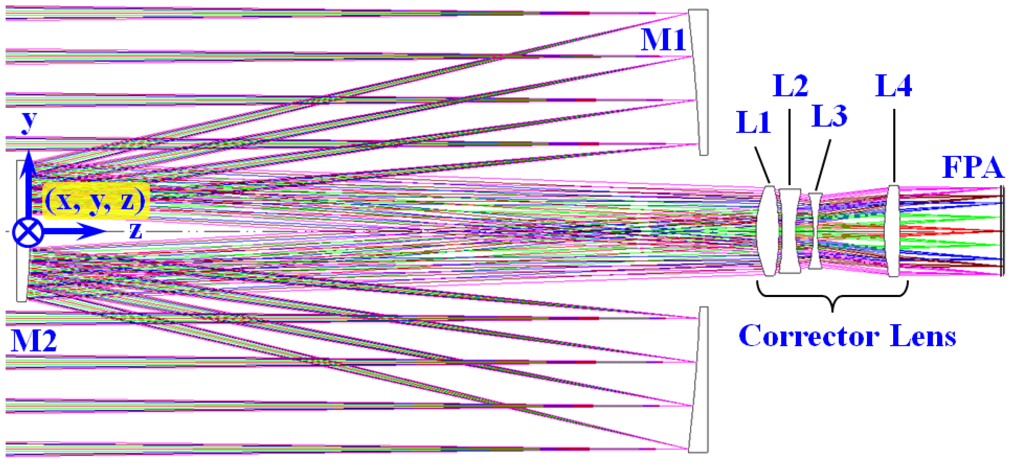
2. Allowable Range of F-Numbers and Design Cases of the Telescope
3. Tolerance of Mirror Elements Versus the F-Number
4. Conclusions
Author Contributions
Funding
Conflicts of Interest
Appendix A

| Design Case | (1) | (2) | (3) | (4) | (5) | (6) | (7) | (8) | (9) | |||||||||||
|---|---|---|---|---|---|---|---|---|---|---|---|---|---|---|---|---|---|---|---|---|
| Pupil Diameter/fn | 800/7.5 | 770/7.8 | 740/8.1 | 710/8.5 | 680/8.8 | 650/9.2 | 620/9.7 | 590/10.2 | 560/10.7 | |||||||||||
| Surface | Type | Material | Radius | Thickness | Radius | Thickness | Radius | Thickness | Radius | Thickness | Radius | Thickness | Radius | Thickness | Radius | Thickness | Radius | Thickness | Radius | Thickness |
| M1 | Conic | ZERODUR | –2770.622 | –998.50 | –2772.368 | –999.27 | –2771.799 | –998.60 | –2771.040 | –998.23 | –2773.306 | –999.32 | –2772.677 | –999.11 | –2772.403 | –997.62 | –2772.582 | –997.58 | –2772.672 | –997.57 |
| Conic Constants | –1.158236204 | –1.158495625 | –1.161542256 | –1.162045757 | –1.1626831 | –1.165604029 | –1.165797514 | –1.169222324 | –1.17032774 | |||||||||||
| M2 | Conic | ZERODUR | –1067.075 | 1079.22 | –1067.331 | 1079.07 | –1068.899 | 1079.08 | –1068.980 | 1077.18 | –1069.105 | 1079.67 | –1068.500 | 1080.70 | –1074.296 | 1080.41 | –1074.880 | 1080.72 | –1075.137 | 1081.14 |
| Conic Constants | –4.662679579 | –4.665672011 | –4.70237211 | –4.709208378 | –4.716077121 | –4.742799171 | –4.766289194 | –4.802887116 | –4.815626274 | |||||||||||
| L1 | Sphere | SILICA | 173.075 | 35.60 | 172.000 | 35.19 | 169.666 | 34.88 | 169.204 | 34.18 | 168.708 | 33.90 | 166.027 | 33.77 | 166.276 | 32.90 | 164.703 | 32.58 | 163.660 | 32.22 |
| Sphere | –362.650 | 6.27 | –363.669 | 5.92 | –359.746 | 5.63 | –363.209 | 5.92 | –359.505 | 6.28 | –345.696 | 5.11 | –358.561 | 6.57 | –353.486 | 6.49 | –349.625 | 6.39 | ||
| L2 | Sphere | SILICA | –396.301 | 20.00 | –402.299 | 20.00 | –403.298 | 20.00 | –408.167 | 20.00 | –400.460 | 20.00 | –385.414 | 20.00 | –403.308 | 20.00 | –400.979 | 20.00 | –396.968 | 20.00 |
| Sphere | 214.798 | 26.42 | 216.256 | 26.97 | 215.456 | 26.41 | 219.428 | 25.24 | 218.517 | 23.58 | 214.096 | 26.50 | 216.042 | 22.06 | 216.187 | 21.00 | 215.816 | 20.80 | ||
| L3 | Sphere | SILICA | –235.739 | 6.00 | –236.312 | 6.00 | –231.928 | 6.00 | –236.334 | 6.00 | –235.304 | 6.00 | –228.056 | 6.00 | –230.529 | 6.00 | –226.726 | 6.00 | –224.828 | 6.00 |
| Sphere | 223.899 | 97.16 | 219.778 | 97.62 | 218.980 | 98.99 | 216.485 | 102.71 | 219.462 | 102.05 | 219.213 | 99.30 | 218.780 | 103.78 | 220.203 | 105.14 | 220.580 | 105.40 | ||
| L4 | Sphere | SILICA | 302.732 | 23.82 | 300.210 | 23.72 | 306.828 | 23.50 | 307.639 | 23.21 | 315.745 | 23.01 | 320.653 | 23.11 | 322.406 | 22.77 | 336.094 | 22.56 | 343.035 | 22.44 |
| Sphere | –1788.857 | 150.00 | –1947.817 | 150.00 | –1790.501 | 150.00 | –2144.501 | 150.00 | –1917.467 | 150.00 | –1473.205 | 150.00 | –1751.763 | 150.00 | –1531.474 | 150.00 | –1419.355 | 150.00 | ||
| Filter | Sphere | SILICA | Infinity | 1.10 | Infinity | 1.10 | Infinity | 1.10 | Infinity | 1.10 | Infinity | 1.10 | Infinity | 1.10 | Infinity | 1.10 | Infinity | 1.10 | Infinity | 1.10 |
| Sphere | Infinity | 2.96 | Infinity | 2.96 | Infinity | 2.96 | Infinity | 3.01 | Infinity | 2.96 | Infinity | 2.96 | Infinity | 2.96 | Infinity | 2.96 | Infinity | 2.97 | ||
| Cover | Sphere | D 263® T | Infinity | 0.70 | Infinity | 0.70 | Infinity | 0.70 | Infinity | 0.70 | Infinity | 0.70 | Infinity | 0.70 | Infinity | 0.70 | Infinity | 0.70 | Infinity | 0.70 |
| Sphere | Infinity | 0.75 | Infinity | 0.75 | Infinity | 0.75 | Infinity | 0.75 | Infinity | 0.75 | Infinity | 0.75 | Infinity | 0.75 | Infinity | 0.75 | Infinity | 0.75 | ||
| Image | FPA | Infinity | –– | Infinity | –– | Infinity | –– | Infinity | –– | Infinity | –– | Infinity | –– | Infinity | –– | Infinity | –– | Infinity | –– | |
References
- Bennett, D.A.; Bell, R.M.; Helmuth, D.B.; Cochrane, A.T.; Miller, T.N.; Lentz, C.A. Remote sensing satellite constellation for world–wide wild fire monitoring. In Proceedings of the Remote Sensing for Environmental Monitoring, GIS Applications, and Geology IX, SPIE Remote Sensing, Berlin, Germany, 7 October 2009; SPIE: Berlin, Germany, 2009; Volume 7478, p. 74780W. [Google Scholar]
- Shack, R.V.; Thompson, K. Influence of alignment errors of a telescope system on its aberration field. In Proceedings of the Optical Alignment I, 24th Annual Technical Symposium, San Diego, CA, USA, 31 December 1980; Shagam, R.M., Sweatt, W.C., Eds.; SPIE: San Diego, CA, USA, 1980; Volume 251, pp. 146–153. [Google Scholar]
- Wilson, R.N.; Delabre, B. Concerning the alignment of modern telescopes: Theory, practice, and tolerances illustrated by the ESO NTT. Publ. Astron. Soc. Pac. 1997, 109, 53–60. [Google Scholar] [CrossRef][Green Version]
- Schmid, T.; Thompson, K.P.; Rolland, J.P. A unique astigmatic nodal property in misaligned Ritchey–Chrétien telescopes with misalignment coma removed. Opt. Express 2010, 18, 5282–5288. [Google Scholar] [CrossRef]
- Yang, H.S.; Lee, Y.W.; Kim, E.D.; Choi, Y.W.; Rasheed, A.A.A. Alignment methods for Cassegrain and RC telescope with wide field of view. In Proceedings of the Space Systems Engineering and Optical Alignment Mechanisms, Optical Science and Technology, the SPIE 49th Annual Meeting, Denver, CO, USA, 30 September 2004; Peterson, L.D., Guyer, R.C., Eds.; SPIE: Denver, CO, USA, 2004; Volume 5528, pp. 334–341. [Google Scholar]
- Hampson, K.M.; Gooding, D.; Cole, R.; Booth, M.J. High precision automated alignment procedure for two–mirror telescopes. Appl. Opt. 2019, 58, 7388–7391. [Google Scholar] [CrossRef] [PubMed]
- Kim, S.; Yang, H.S.; Lee, Y.W.; Kim, S.W. Merit function regression method for efficient alignment control of two–mirror optical systems. Opt. Express 2007, 15, 5059–5068. [Google Scholar] [CrossRef]
- Lee, H.; Dalton, G.B.; Tosh, I.A.; Kim, S.W. Computer–guided alignment II: Optical system alignment using differential wavefront sampling. Opt. Express 2007, 15, 15424–15437. [Google Scholar] [CrossRef]
- Oh, E.; Ahn, K.B.; Kim, S.W. Experimental sensitivity table method for precision alignment of Amon–Ra instrument. J. Astron. Space Sci. 2014, 31, 241–246. [Google Scholar] [CrossRef]
- Abitbol, M.H.; Ahmed, Z.; Barron, D.; Basu Thakur, R.; Bender, A.N.; Benson, B.A.; Bischoff, C.A.; Bryan, S.A.; Carlstrom, J.E.; Chang, C.L.; et al. Telescope engineering to control systematic errors. In CMB–S4 Technology Book, 1st ed.; ArXiv: Ithaca, NY, USA, 2017; pp. 14–16. [Google Scholar]
- O’Neill, E.L. Transfer function for an annular aperture. J. Opt. Soc. Am. 1956, 46, 285–288. [Google Scholar] [CrossRef]
- Wilson, R.N. Reflecting Telescope Optics I Basic Design Theory and its Historical Development, 2nd ed.; Springer: New York, NY, USA, 2007; pp. 319–320. [Google Scholar]
- Smith, W.J. Modern Optical Engineering, 4th ed.; McGraw–Hill Education: New York, NY, USA, 2008; pp. 392–397. [Google Scholar]
- King, W.B. Use of the modulation–transfer function (MTF) as an aberration–balancing merit function in automatic lens design. J. Opt. Soc. Am. 1969, 59, 1155–1158. [Google Scholar] [CrossRef]
- Synopsys. CODE V®, Synopsys: Mountain View, CA, USA, 2019.
- Hopkins, H.H.; Tiziani, H.J. A theoretical and experimental study of lens centring errors and their influence on optical image quality. Br. J. Appl. Phys. 1966, 17, 33–54. [Google Scholar] [CrossRef]
- Rimmer, M. Analysis of perturbed lens systems. Appl. Opt. 1970, 9, 533–538. [Google Scholar] [CrossRef] [PubMed]
- Rimmer, M. A tolerancing procedure based on modulation transfer function (MTF). In Proceedings of the Computer–Aided Optical Design, 22nd Annual Technical Symposium, San Diego, CO, USA, 1 December 1978; SPIE: San Diego, CA, USA, 1978; Volume 147, pp. 66–70. [Google Scholar]
- Koch, D.G. A statistical approach to lens tolerancing. In Proceedings of the Computer–Aided Optical Design, the 22nd Annual Technical Symposium, San Diego, CA, USA, 1 December 1978; SPIE: San Diego, CA, USA, 1978; Volume 147, pp. 71–82. [Google Scholar]
- Bely, P.Y. The Design and Construction of Large Optical Telescopes, 1st ed.; Springer: New York, NY, USA, 2002; pp. 9–18. [Google Scholar]
- Ginsberg, R.H. Outline of tolerancing (from performance specification to toleranced drawings). Opt. Eng. 1981, 20, 175–180. [Google Scholar]


| Parameters | Description |
|---|---|
| Spectral Range | 400–900 nm |
| Filter Bands | 2 Panchromatic + 6 Multi-Spectral |
| Sensor Pixel Pitch/Resolution | Pan.: 7 μm/12,000 pixel, M.S.: 28 μm/3000 pixel |
| Ground Sampling Distance | 0.7 m/pixel @ 600 km of Altitude; Sun-Synchronous Orbit |
| Field of View | >1° (Diagonal) |
| Swath Width | >8.4 km |
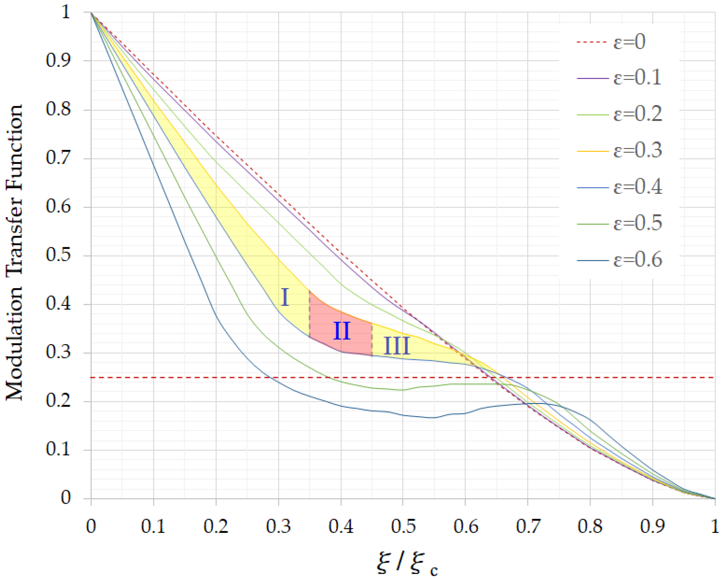
| Optical MTF | As–Built ≥ 0.25 @ 71.429 lp/mm, Panchromatic; 18 lp/mm, Multi-Spectral |
| ξ/ξc | ξc = 1/(λ⋅ fn) | fn |
|---|---|---|
| 0.35 | 204.1 | 7.7 |
| 0.36 | 198.4 | 8.0 |
| 0.37 | 193.1 | 8.2 |
| 0.38 | 188.0 | 8.4 |
| 0.39 | 183.2 | 8.6 |
| 0.40 | 178.6 | 8.8 |
| 0.41 | 174.2 | 9.1 |
| 0.42 | 170.1 | 9.3 |
| 0.43 | 166.1 | 9.5 |
| 0.44 | 162.3 | 9.7 |
| 0.45 | 158.7 | 10.0 |
| Design Case | (1) | (2) | (3) | (4) | (5) | (6) | (7) | (8) | (9) |
|---|---|---|---|---|---|---|---|---|---|
| Pupil Diameter/fn | 800/7.5 | 770/7.8 | 740/8.1 | 710/8.5 | 680/8.8 | 650/9.2 | 620/9.7 | 590/10.2 | 560/10.7 |
| min. MTF | 0.39 | 0.37 | 0.36 | 0.36 | 0.34 | 0.33 | 0.32 | 0.31 | 0.30 |
| Distortion (%) | 0.149 | 0.149 | 0.149 | 0.148 | 0.149 | 0.149 | 0.149 | 0.149 | 0.150 |
| Chief Ray Angle (°) | 2.63 | 2.63 | 2.63 | 2.60 | 2.63 | 2.63 | 2.63 | 2.62 | 2.62 |
| Obstruction Ratio | 0.325 | 0.338 | 0.341 | 0.344 | 0.347 | 0.348 | 0.355 | 0.356 | 0.357 |
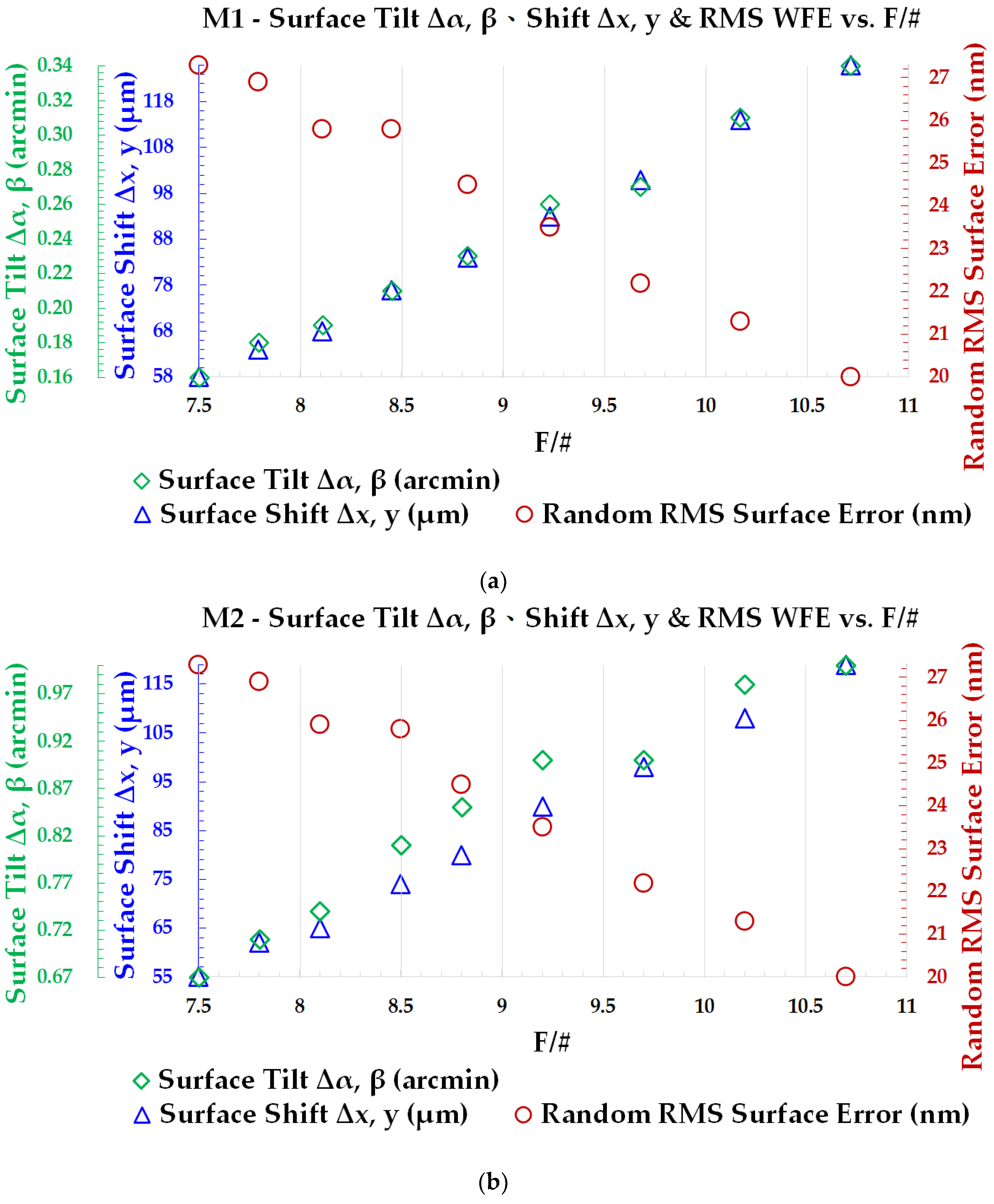
| fn | M1 & M2 RMS Surface WFE (nm) | Primary Mirror, M1 Surface | Secondary Mirror, M2 Surface | ||
|---|---|---|---|---|---|
| Tilt Error Δα, Δβ (arcmin) ** | De-Center Δx, Δy (μm) * | Tilt Error Δα, Δβ (arcmin) ** | De-Center Δx, Δy (μm) * | ||
| 7.5 | 27 | 0.16 | 58 | 0.67 | 55 |
| 7.8 | 27 | 0.18 | 64 | 0.71 | 62 |
| 8. | 25 | 0.19 | 68 | 0.74 | 65 |
| 8.5 | 25 | 0.21 | 77 | 0.81 | 74 |
| 8.8 | 24 | 0.23 | 84 | 0.85 | 80 |
| 9.2 | 23 | 0.26 | 93 | 0.90 | 90 |
| 9.7 | 22 | 0.27 | 101 | 0.90 | 98 |
| 10.2 | 21 | 0.31 | 114 | 0.98 | 108 |
| 10.7 | 20 | 0.34 | 126 | 1.04 | 119 |
| Tolerance Type | Primary Mirror, M1 Surface | Secondary Mirror, M2 Surface |
|---|---|---|
| RMS Surface WFE (nm) | 22 | 22 |
| De-center Δx, Δy (μm) | 98 | 98 |
| Tilt error Δα, Δβ (arcmin) | 0.26 | 0.90 |
© 2020 by the authors. Licensee MDPI, Basel, Switzerland. This article is an open access article distributed under the terms and conditions of the Creative Commons Attribution (CC BY) license (http://creativecommons.org/licenses/by/4.0/).
Share and Cite
Lin, S.-F.; Chen, C.-H.; Huang, Y.-K. Optimal F-Number of Ritchey–Chrétien Telescope Based on Tolerance Analysis of Mirror Components. Appl. Sci. 2020, 10, 5038. https://doi.org/10.3390/app10155038
Lin S-F, Chen C-H, Huang Y-K. Optimal F-Number of Ritchey–Chrétien Telescope Based on Tolerance Analysis of Mirror Components. Applied Sciences. 2020; 10(15):5038. https://doi.org/10.3390/app10155038
Chicago/Turabian StyleLin, Sheng-Feng, Cheng-Huan Chen, and Yi-Kai Huang. 2020. "Optimal F-Number of Ritchey–Chrétien Telescope Based on Tolerance Analysis of Mirror Components" Applied Sciences 10, no. 15: 5038. https://doi.org/10.3390/app10155038
APA StyleLin, S.-F., Chen, C.-H., & Huang, Y.-K. (2020). Optimal F-Number of Ritchey–Chrétien Telescope Based on Tolerance Analysis of Mirror Components. Applied Sciences, 10(15), 5038. https://doi.org/10.3390/app10155038