Article

Development Cycle Modeling: Resource Estimation

1
Fortify, Micro Focus International plc, Houston, TX 77027, USA
2
Department of Mechanical Engineering, Texas Tech University, Lubbock, TX 79409, USA
3
Department of Computer Science, Texas Tech University, Lubbock, TX 79409, USA
*
Author to whom correspondence should be addressed.
Appl. Sci. 2020, 10(14), 5013; https://doi.org/10.3390/app10145013
Submission received: 1 June 2020 / Revised: 2 July 2020 / Accepted: 7 July 2020 / Published: 21 July 2020

Abstract

:
This paper presents results produced by a domain-independent system development model that enables objective and quantitative calculation of certain development cycle characteristics. The presentation recounts the model’s motivation and includes an outline of the model’s structure. The outline shows that the model is constructive. As such, it provides an explanatory mechanism for the results that it produces, not just a representation of qualitative observations or measured data. The model is a Statistical Agent-based Model of Development and Evaluation (SAbMDE); and it appears to be novel with respect to previous design theory and methodology work. This paper focuses on one development cycle characteristic: resource utilization. The model’s resource estimation capability is compared to Boehm’s long-used software development estimation techniques. His Cone of Uncertainty (COU) captures project estimation accuracy empirically at project start but intuitively over a project’s duration. SAbMDE calculates estimation accuracy at start up and over project duration; and SAbMDE duplicates the COU’s empirical values. Additionally, SAbMDE produces results very similar to the Constructive Cost Model (COCOMO) effort estimation for a wide range of input values.

1. Introduction

A development cycle model represents the phases of system and/or product development. There are many such models currently in use. For example, Microsoft offers their Security Development Lifecycle [1,2]. The National Institute of Standards and Technology (NIST) and other government organizations specify standards and instructions [3,4] that are necessarily incorporated by industry [5,6]. Researchers such as [7], have often enumerated and compared various methodologies. However, all these models and methodologies represent a developer’s effort to convert an idea into an end product. The models describe the intermediate requirement, design, and implementation phases as well as the testing phase that maintains the integrity of the conversion process. Figure 1 illustrates this representation in broad terms.
The conventional models are usually expressed as best practices, guidance, and policies [8,9]. For that reason, the models’ effectiveness depends strongly on the skill and will of the developers who interpret and execute the models [10]. The models are qualitative; it is difficult to apply them objectively and consistently. Many quantitative function- and/or phase-specific sub-models exist: software reliability growth modes (SRGM) [11], technical debt [12], run-time behavior extraction [13,14], and more. However, the sub-models typically measure output from an existing system. Consequently, they analyze history rather than predict possibilities. In addition, the sub-models represent development phases differently, so differently that the idea of an end-to-end development cycle model has seemed out of reach. Even so, there is some consensus in the design theory and methodology (DTM) community that a phase-independent underlying model exists. The literature reviews [15,16] state this consensus; and [17] describes the evolution of that consensus. There is also evidence of this thinking outside of the DTM community. For example, while formulating a theoretical foundation for building construction, Antunes and Gonzalez [18] state, “In this research, construction is not restricted to civil engineering and architecture, but comprehends a broader understanding of building, putting up, setting up, establishing and assembling. Construction is the materialization of a concept through design, taking into account functional requirements and technical specifications for a project product utilizing specialized labour.” Antunes and the Statistical Agent-based Model of Development and Evaluation (SAbMDE) both envision underlying domain-independent models. The Defense Advanced Research Projects Agency (DARPA) is one of the organizations that fuels renewed interest in the underlying model by soliciting the research results [19,20,21,22] that such a model might promise. The increasing complexity of modern systems [23,24] is a major reason for the renewal.

2. Proposed Model

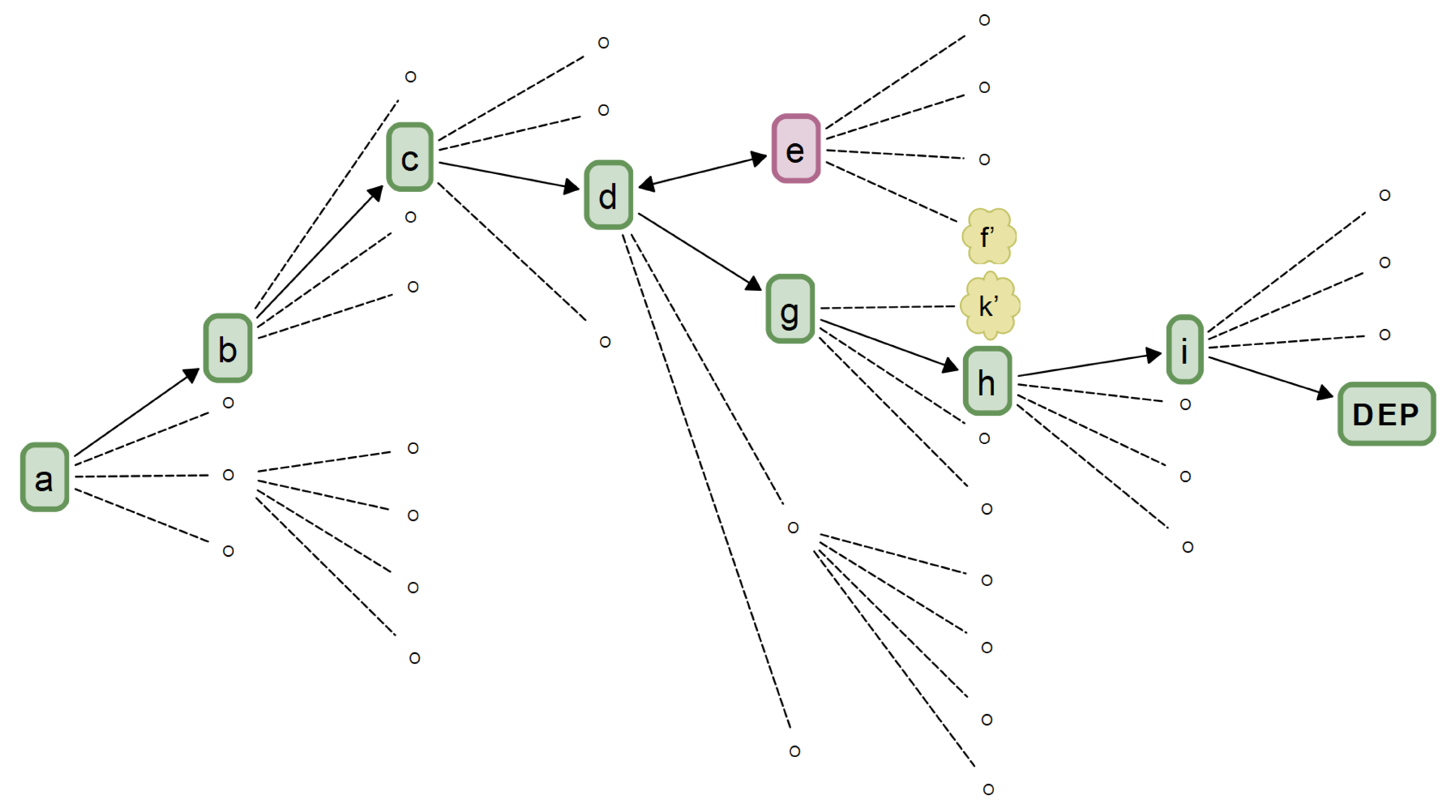
Figure 1 also illustrates an underlying model candidate: the Statistical Agent-based Model of Development and Evaluation (SAbMDE). SAbMDE joins with those [25] who accept development as an inherently human process and builds on a neuroscience foundation [26,27,28] of agent mind, body, and environment interaction. SAbMDE then uses process algebra ideas, such as Wang’s [29,30], to represent each development phase so that analytical techniques can be uniformly applied across the entire development cycle. Wang has shown [31] that a desired end product (DEP) can be developed by sequentially composing intermediate products (IP) from sets of fundamental composable elements: processes and relations. SAbMDE introduces an agent who decides which elements to compose. A correct decision set produces a sequence of compositions that become an end product, hopefully, the DEP. SAbMDE recognizes (a) that each decision is one of a set of alternatives, (b) that the hierarchical super-set of alternatives forms a development space (DSpace), and (c) that the correct DEP decision set is the best of many development paths (DPaths) through DSpace. The model’s foundation reflects itself in this representation via three inter-related sub-models: Agent, Development, and Evaluation. Model D houses the algorithms and structures that quantitatively define DSpace as well as the tools for DSpace navigation and traversal. Model E contains the testing and evaluation mechanism that informs the decisions that compel DSpace compositions. Model A emulates a development agent’s perception, experience, vocabulary, and other human factors needed to create the Model E tests and to evaluate their results. Because each DSpace composition is connected by a decision to an evaluation of test results, there is an ESpace that mirrors DSpace. Because each ESpace test and/or evaluation maps to an agent’s perception and vocabulary, there is an ASpace that mirrors ESpace. These spaces, generically XSpaces, have the same form and share a mathematical description. When executed together, Models A, D, and E represent a development cycle quantitatively and flexibly. This capability allows SAbMDE to hypothesize that DSpace characteristics constrain and guide an agent’s decision-making in ways that conventional development cycle models can not. SAbMDE constructs DSpace from sets of composable elements: vocabulary items, V, and relations, R. For example, (1) and (2) are the basis of the simple DSpace fragment in Figure 2. Composable elements are supplied directly by an agent or extracted from documents by simple parsing or more sophisticated techniques such as those applied by Park and Kim [32].
V = { v 0 , v 1 , v 2 , v 3 }
R = { r 0 }
The construction begins at composition index 0 ( l = 0 ) with an empty set. Construction continues by enumerating the composable elements at l = 1 , and then by using the cross-product operator to compose all the combinations of composable elements for l > 1 . As a result, at every DSpace node (DNode) for l > 1 , an agent decision-maker has exactly | V | | R | options from which to choose. Note that at l = 1 , only the vocabulary items are listed because composition is the same as vocabulary item selection at this composition index; relations have been enumerated but not applied. DSpace is characterized by the choice of composable elements, the numbers of types of composable elements, | V | and | R | ), and the number of compositions, L, required to produce the DEP.
A development agent navigates or traverses DSpace by deciding which DNode to compose next. Figure 2 shows a DPath. Note that the DPath is not a direct one. The decision to traverse to DNode e was a mistake that had to be corrected. An evaluation of DNodes f and k confirmed the error. Thus, the actual DPath is contorted. At each DNode, the structure of DSpace offers a probability floor for the agent’s likelihood of making a successful decision, i.e., one that leads to the DEP. Those floor values are defined by (3)–(5); and they correspond to random choices. In real situations, agents act with some level of skill. To recognize this skill, the DNode probabilities are scaled with a 0–10 (random–perfect) index, f s , as in (6).
p ( l ) = 0 , l = 0 1 | V | , l = 1 1 | V | | R | , l > 1
u = 1 | V |
q = 1 | V | | R | = 1 Q
p = x + f s 10 ( 1 x ) , f s = 0 , 1 , . . . 10 and x = u or q
With this brief outline and with the details to follow, SAbMDE proposes to quantitatively model development processes. This paper supports that proposal by focusing on one aspect of that modeling: resource estimation.

3. Related Work

Resource estimation is critical to any project management effort; and, as might be expected, there is a rich history of modeling efforts to make estimates accurately and efficiently. This is certainly true in the software development domain. Several researchers, e.g., [33,34,35,36], have compared, cataloged, and categorized the various software estimation methods. The categories include model-based, expertise-based, learning-oriented, dynamics-based, regression, and Bayesian. Over time, researchers have explored these techniques extensively. Trendowicz has even defined a set of requirements that should be considered when selecting an estimation method. Having done so, he states, “An analysis of existing estimation methods with respect to industrial objectives and derived requirements indicates a few leading methods that meet most of the requirements; although no single method satisfies all requirements.
Unfortunately, the results of the researchers’ comparisons are also not encouraging. For example, Trendowicz [34] concludes, “The discrepancy between what is needed by the software industry and what is actually provided by the research community indicates that further research should, in general, focus on providing estimation methods that keep up with current industrial needs and abilities.” And, Boehm et al. [33] conclude, “The important lesson to take from this paper is that no one method or model should be preferred over all others. The key to arriving at sound estimates is to use a variety of methods and tools and then investigating the reasons why the estimates provided by one might differ significantly from those provided by another.” Basha and Dhavachelvan [37] agree with Boehm: “The primary conclusion is that no single technique is best for all situations, and that a careful comparison of the results of several approaches is most likely to produce realistic estimates.
Vera et al. [35] approach the estimation method selection problem from a different angle. They attempt to identify a taxonomy so that would-be estimators can speak clearly about the methodological options available to them. In answer to their first research question (RQ1) about Software Development Estimation (SDEE), they conclude, “Concerning the RQ1 this work determined that there is not a widely accepted taxonomy, since there are too many relevant and almost independent criteria to classify the SDEE techniques. Moreover, the hierarchical structure used to represent the taxonomies is not much useful to help identify clusters of techniques potentially useful for a software organization. This is probably true also to organize the knowledge in this study domain.
There appears to be a consensus that the state-of-the-art of software effort estimation is not ideal. The implication is that a better effort estimation method is needed.

4. Results

This paper hypothesizes that one characteristic of the proposed model is the ability to compute the effort required to complete a project. In the language of the proposed model, completing a project is traversing a DSpace along a DPath that leads to a DEP. This section derives and describes the methods and calculations needed to make the traversal. After this section, the calculations are discussed; and then conclusions are drawn.
The estimation calculations are presented in four parts. First is the definition of the components of a resource estimation calculation: DSpace traversal, a pricing scheme, and the cost computation procedure. Then, SAbMDE resource estimation results are compared to the empirically-derived Constructive Cost Model (COCOMO) [38] effort estimation results.

4.1. DSpace Traversal

The ideal traversal of a DSpace to a specified DEP requires a sequence of L correct composition decisions. What is an agent’s likelihood of making L correct decisions in a row? The structure of DSpace is a graph, a tree, that defines the minimal probability of a correct decision. At any DNode, that probability is the inverse of an agent’s choice of DPath alternatives as in (3). Because, at each DNode, an agent’s next-node traversal decision is independent of any previous such decision [39], a DPath can be treated like a Markov Chain. The Markov Chain probability is described by (7) and, after insertion of (3), by (8).
p ( L ) = p ( 1 ) l = 2 L p ( l | ( l 1 ) ) )
p ( l ) = | V | ( 2 l + 1 ) | R | ( 2 l + 3 )
After substitution of simplifying transforms, (4) and (5), the Markov Chain probability becomes (9).
p ( l ) = u 2 q ( 2 l 3 )
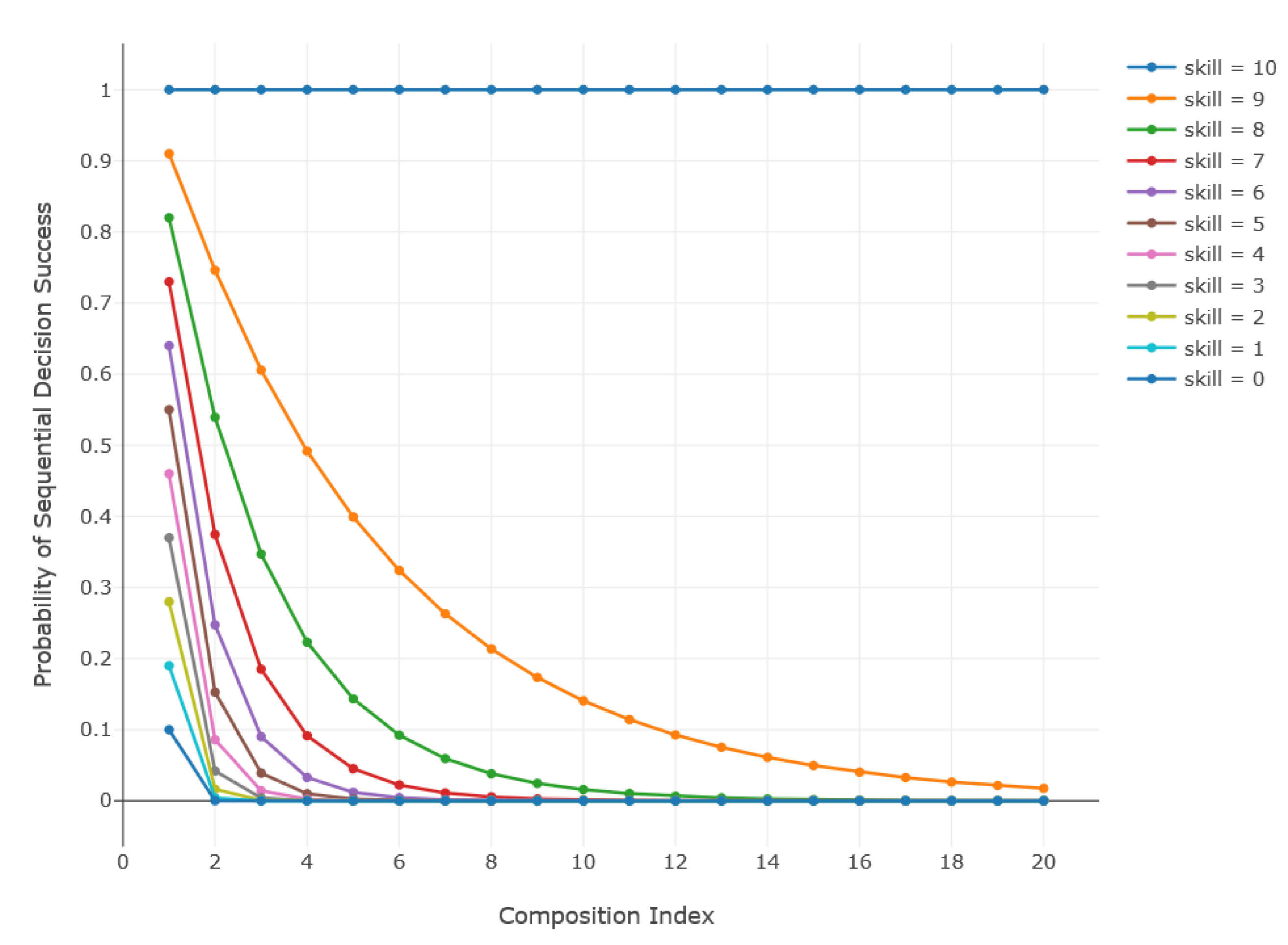
Figure 3 is a graph of (9) scaled with (6). It shows that, in all but the case of the perfect decision-maker, the likelihood of successfully traversing a DEP DPath is low. Even the skill index 9 agent has only a 50% chance of getting four sequential decisions correct. It is clear that every agent that attempts a DSpace traversal will make mistakes, some more than others. This is not an unexpected result. One implication is that only agents with maximum skill should be decision-makers. Another implication is that whatever method an agent uses to make a decision should be re-calibrated frequently to prevent the agent from sliding down the multi-decision probability curve.

4.2. SAbMDE Resource Utilization

Begin an estimate of the resource utilization associated with a DPath by assigning a price to each vocabulary item and relation. Then, with an appropriate function, assign a price to the act of their composition. Similarly, assign a price to their decomposition. The definitions and equations below describe a simple pricing system.
P v = vocabulary item price , actual or normalized P r = relation price , actual or normalized g c p ( P v , P r ) = composition pricing function g d p ( P v , P r ) = decomposition pricing function f b = backtrack factor l b = backtrack length n = number of decision re-tries
g c p ( P v , P r ) = ( P v + P r )
g d p ( P v , P r ) = f b g c p ( P v , P r )
P = g c p + ( n 1 ) l b g d p
Finally, calculate a DPath’s resource utilization by summing the composition prices for each product in the DPath. Such a summation for as-yet untraversed portions of the DPath is an estimate of the resources to be utilized. As noted previously, only a perfect agent can make the perfect decision set to reach a DEP. All other agents will make incorrect decisions. Of course, agents must attempt to complete a project; so when an agent discovers an incorrect decision, they will likely undo that decision and try again. The number of retries is a function of the agent’s skill index and the number of alternative choices as defined by the DSpace. An agent retries by selecting one of the alternatives, evaluating the selection, and again discarding incorrect selections. The hypergeometric distribution [40] in (13) can describe this process.
p c ( k m ) = K M k m M K M m k m M m
where
M = | V | | R | , K M = M p s k i l l , k m = 0
The (13) variables are interpreted as follows. For each skill index, there is a probability, p s k i l l , of making a correct decision. For a decision population size, M, p s k i l l is equivalent to having a correct decision population size, K M . Given these values, the hypergeometric distribution can calculate the probability that a sample of size m will have k m correct decisions. Setting k m = 0 and choosing a small probability criterion, p c ( k m ) , corresponds to calculating an upper limit on the number of retries, n = k m , that will guarantee a correct decision. Table 1 is an excerpted example of this calculation for a p s k i l l corresponding to skill index=0, M = 100 , K M = 1 , and a 0.1 probability criterion, p c ( k m ) . The table shows that as many as 90 retries are required to ensure a 90% chance of decision success.
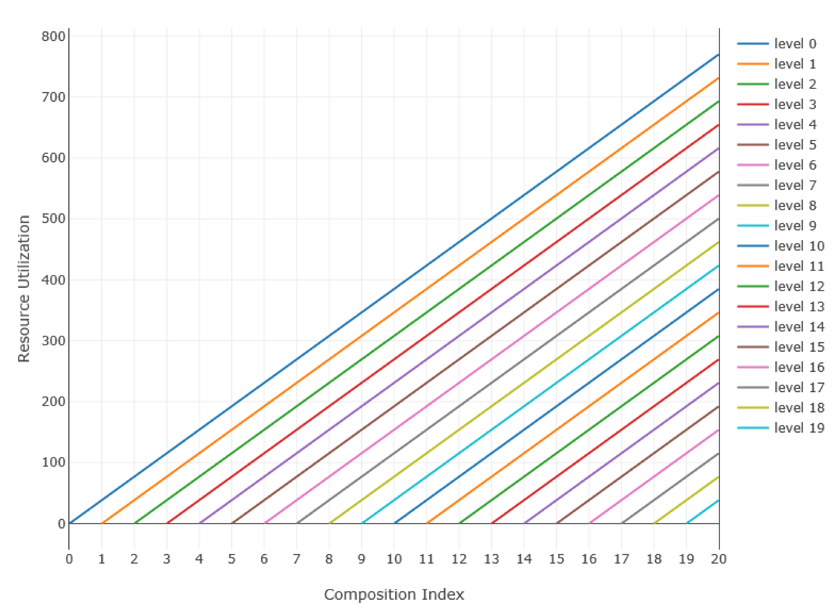
When an agent makes an incorrect decision, the agent may continue on the incorrect DPath for some number of compositions. Once the error is discovered, the agent will likely return to the last correct decision and retry; and the no longer needed compositions will be decomposed during the return trip. Equations (11) and (12) handle the added resource utilization with the backtrack length and backtrack factor parameters. The latter assumes that the price of composition and decomposition differ. Figure 4 shows resource utilization estimates calculated as described above. These estimates were calculated using skill index 7, with vocabulary item and relation prices of 1 and 10, respectively, and with backtrack length and backtrack factor values of 1 and 1.5, respectively. In keeping with the last Markov Chain implication noted above, estimates are repeated at each composition index of the 20-composition project.
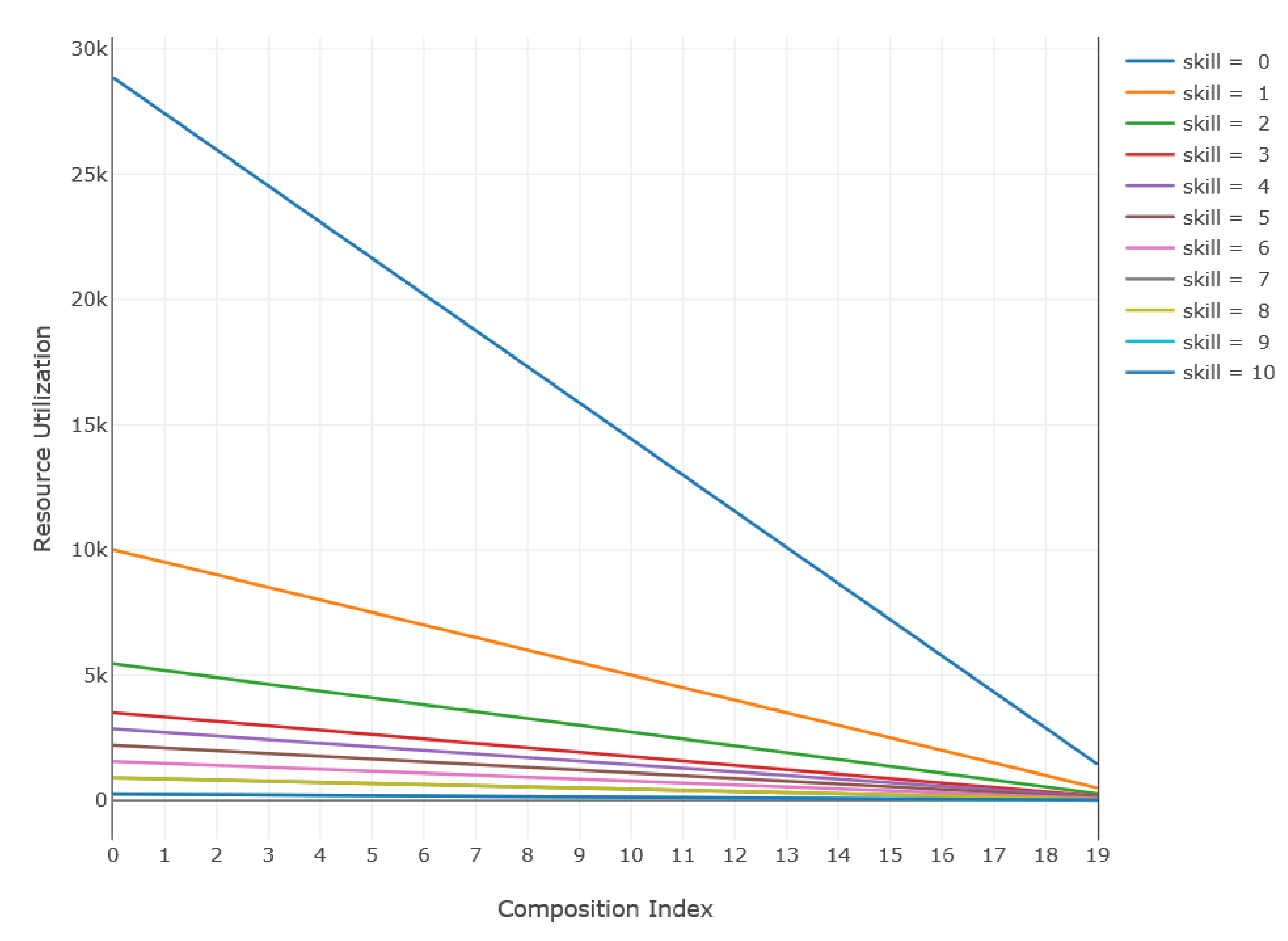
For each graph trace, the resource utilization value on the far right ( l = 19 ) is the estimate for the remainder of the project as viewed from the composition index of the origin of the trace. When only those far right values were plotted as a function of their origins ( l = 0 , 1, 2, …), they appear as shown in Figure 5 which includes estimates for each skill index.
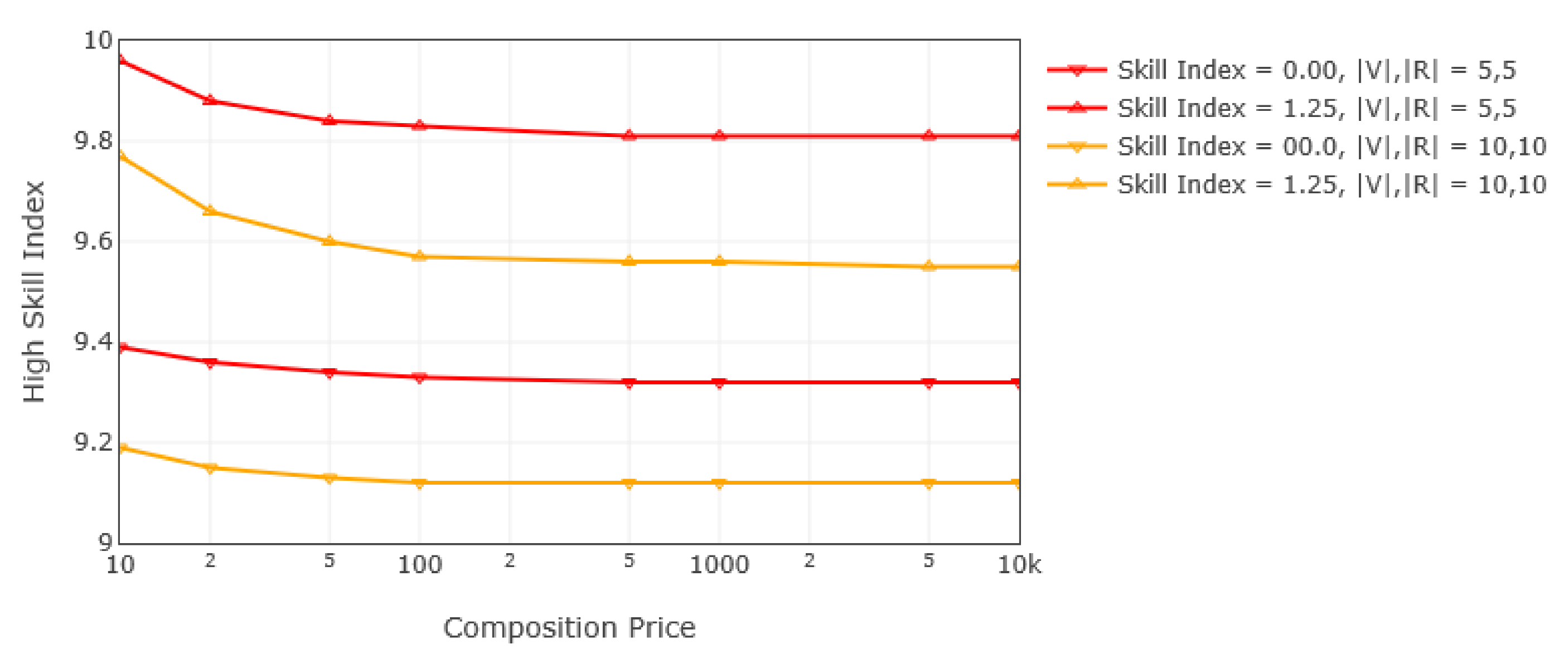
Table 2 shows that, at composition index 0, the high skill index estimate values are approximately 16 times the low estimate values. The Figure 5 estimates were computed with vocabulary item and relation prices of 5 and 8 respectively. Figure 6 shows the 16:1 skill indices computed for other prices. It shows that these indices vary only slightly with price, and even then, only at the smallest prices.
When the 16:1 ratio skill index calculation is done with fixed price but with varying backtrack parameter values, as in Table 3, there is also only a slight variation.
The 16:1 ratio of high to low estimate values as a function of skill index, as revealed by the effort estimation procedure, appears to be a nearly invariant characteristic of DSpace.

4.3. COCOMO Effort Estimation

The 16:1 ratio is noteworthy because it is very similar to empirical data captured in Boehm’s [41] (p. 311) Cone of Uncertainty (COU). This similarity encourages additional comparison with COCOMO estimation [38]. Equations (14) and (15) are the COCOMO effort estimation formula that computes the Person-Months ( P M ) required by a project. The formula is an exponential regression curve based on code size and other variables derived from analysis of project data. Code size, S i z e , is measured in thousands of lines of source code (KLOC).
P M N S = A ( S i z e E ) i = 1 n h E M i
where E = B + 0.01 j = 1 5 S F j
The project-related Scale Factors ( S F ) and the developer-related Effort Multipliers ( E M ) are computed from subjective data. An estimator observes, surveys, and otherwise gathers data that is then ranked with the scales in Table 4 and Table 5. The regression parameters A through E calibrate the model to the available data. Table 6 and Table 7 show values calibrated to the COCOMO data set.
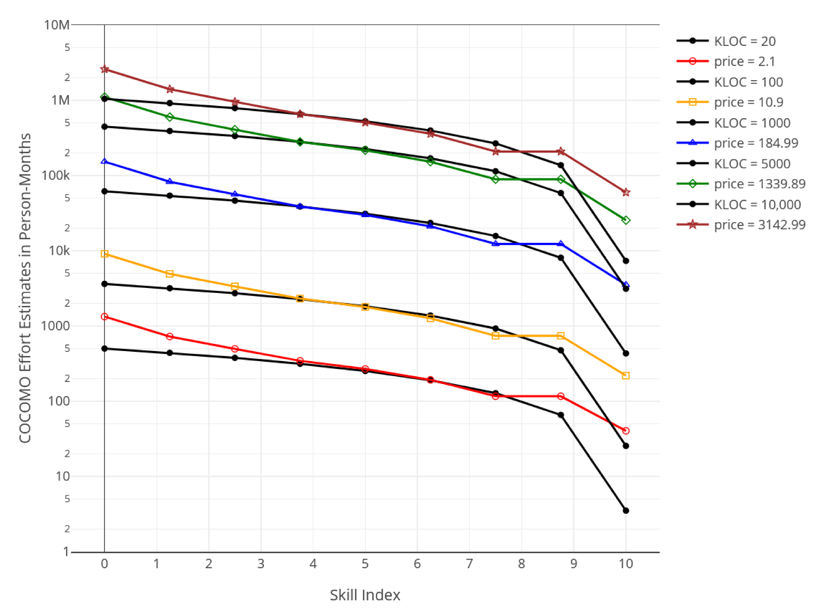
Figure 7 shows COCOMO estimates calculated with the parameters above and for a range of code sizes. In anticipation of comparison with SAbMDE estimates, only the upper limit estimate values, those for E = 1.23 , were plotted.

4.4. SAbMDE–COCOMO Comparison

The successful comparison of SAbMDE resource utilization and COCOMO effort estimates requires a slight adjustment of the independent variable that indexes the SAbMDE resource utilization values. For SAbMDE, skill index = 0 indicates that an agent makes random composition decisions; whereas skill index = 10 indicates perfect decisions. However, for COCOMO, skill index = 0 indicates a minimal (non-random) level of skill whereas skill index = 10 indicates a maximum skill level that is less than perfect. This was described by Boehm [38] (p. 31), e.g., “Analyst teams that fall in the fifteenth percentile are rated very low and those that fall in the ninetieth percentile are rated as very high.” To resolve these scaling differences, SAbMDE skill indices 0 and 10 were removed. SAbMDE skill indices 1 and 9 were matched to COCOMO skill indices 0 and 10; and the remaining SAbMDE skill index intervals were stretched by 10/8 to fit the new end points. The result of this adjustment is shown inTable 8. The new 9-point scale now has the same meaning for both SAbMDE and COCOMO estimate values. Table 8 also shows the corresponding Scaled E M values.
When the Figure 7 COCOMO and SAbMDE estimates are recalculated with their corresponding adjusted skill indices, the estimates can be compared confidently. The comparison, COCOMO with SAbMDE estimates overlaid, is shown graphically in Figure 8.
The SAbMDE and COCOMO estimates, S i and C i , were closely matched by setting initial composable element prices, g c p ( 1 , 1 ) from (10), and then incrementally increasing those prices until the estimates’ mean sum of differences (MSD) were minimized using (16). The minimization was performed with a simple brute force technique. The minimization target on the right-hand side of (17) is calculated by applying a minimization criterion, ε , to the mean sum of the COCOMO estimate for a given KLOC value. For example, ε = 0.1 .
m s d = 1 N i = 0 N | C i S i |
m s d ε N i = 0 N | C i |
The SAbMDE and COCOMO estimates compare favorably over their common skill index ranges. They compare even more favorably over a central range, skill index from 3 to 7; and it was this central range that was used for the MSD matching.

5. Discussion

The estimate correlations are important; but other factors should also be considered. On one hand, COCOMO is a well thought out curve fit to a well-known, long-used data set. Using COCOMO is a matter of gathering information about a project in its very earliest stages, casting that data in terms of the COCOMO regression parameters, and taking into account any differences between the COCOMO data set projects and the project being estimated. Once this is done, the actual calculation takes seconds to complete. The results assume that the estimate is made at the beginning of the project. Also, the results are designed to apply to projects that use the Waterfall or the Spiral development methodology [38] (p. 44). On the other hand, using SAbMDE requires an agent to select the number of compositions to represent the current project at its current maturity level, to enumerate the composable elements associated with those compositions, and then to assign prices to the composable elements. Once this is done, the actual calculation takes seconds to complete. The calculation can adjusted easily as the current project evolves. An estimate can be performed as frequently as needed. The results are methodology-agnostic. SAbMDE is a work in progress. Further mathematical and software development is necessary. Although the model reproduces COCOMO results quite well and has been shown to match certain accepted characteristics of other design theories, additional validation is necessary and underway. Because the modeling concept is new and because user interface requirements are challenging, practical deployment of the model could be problematic; however, these issues are being given due consideration.

6. Conclusions

The focus of this work has been development resource estimation. This work has demonstrated that a constructive technique for estimating development resource utilization is possible and that it produces results very similar to the COCOMO technique currently used for software development. A constructive technique has the advantage of allowing its user to understand the mechanism by which its results were generated. However, SAbMDE has demonstrated several additional benefits. It calculates using the current project’s characteristics, not historical values of other projects. It can be applied and re-applied throughout the development cycle to ensure use of the most current project data. It identifies project prediction limits and calculates project resource utilization bounds. Its input can be captured more objectively. SAbMDE does not depend on a specific development methodology.

Author Contributions

This paper was written from S.D.’s Ph.D. dissertation. A.E., the advisor of S.D., helped draft preparation of the article. S.M. and S.E.-O., S.D.’s committee members helped with reviewing and editing of the article. All authors have read and agreed to the published version of the manuscript.

Funding

This research received no external funding.

Conflicts of Interest

The authors declare no conflict of interest.

Abbreviations

SymbolsDefinitions
C i COCOMO estimate values
ε msd minimization criterion
f b backtrack factor, the ratio of decomposition to composition price
f s skill index value
g c p function that computes the price of composition
g d p function that computes the price of decomposition
k m hypergeometric distribution tagged sample size
K M hypergeometric distribution tagged population size
lcomposition index
l b backtrack length, the number of incorrect compositions performed after a bad
decision and prior to recognition of that bad decision; conversely, the number of
decompositions required to be back on track.
Lnumber of composition levels needed to compose a DEP
m s d mean sum of differences
mhypergeometric distribution sample size
Mhypergeometric distribution population size
nnumber of retries needed to select the correct DNode
Nnumber of skill index values over which m s d summation is averaged
pgeneric probability variable
p c hypergeometic distribution decision probability criterion
P r relation price
p s k i l l probability associated with a skill index value
P v vocabulary item price
qprobability associated with DNode selection
Qproduct of V and R
Rset of relations
rmember of the set of relations
S i SAbMDE estimate values
s k i l l , s k i l l i n d e x index with range [0, 10] that ranks an agent’s skill level, see f s
uprobability associated with vocabulary item selection
vmember of the set of vocabulary items
Vset of vocabulary items
xplaceholder variable

References

  1. Howard, M.; Lipner, S. The Security Development Lifecycle; Secure Software Deelopment, Microsoft Press: Redmond, WA, USA, 2006; p. 320. [Google Scholar]
  2. Microsoft. Simplified Implementation of the Microsoft SDL. Available online: https://www.microsoft.com/en-us/securityengineering/sdl/ (accessed on 3 May 2020).
  3. NIST Special Publication 800-37 Revision 2. Risk Management Framework for Information Systems and Organizations. Department of Commerce p183. Available online: https://doi.org/10.6028/NIST.SP.800-37r2 (accessed on 23 May 2020).
  4. Systems Engineering Life Cycle Department of Homeland Security: P 15. Available online: https://www.dhs.gov/sites/default/files/publications/Systems%20Engineering%20Life%20Cycle.pdf (accessed on 23 May 2020).
  5. Seal, D.; Farr, D.; Hatakeyama, J.; Haase, S. The System Engineering Vee is it Still Relevant in the Digital Age? In Proceedings of the NIST Model Based Enterprise Summit 2018, Gaithersburg, MD, USA, 4 April 2018; p. 10. [Google Scholar]
  6. FHWA. Systems Engineering for ITS Handbook—Section 3 What is Systems Engineering? Available online: https://ops.fhwa.dot.gov/publications/seitsguide/section3.htm (accessed on 3 May 2020).
  7. Modi, H.S.; Singh, N.K.; Chauhan, H.P. Comprehensive Analysis of Software Development Life Cycle Models. Int. Res. J. Eng. Technol. 2017, 4, 5. [Google Scholar]
  8. Sedmak, A. DoD Systems Engineering Policy, Guidance and Standardization. In Proceedings of the 19th Annual NDIA Systems Engineering Conference, Springfield, VA, USA, 26 October 2016; p. 21. Available online: https://ndiastorage.blob.core.usgovcloudapi.net/ndia/2016/systems/18925-AileenSedmak.pdf (accessed on 1 June 2020).
  9. Systems Engineering Plan Preparation Guide. Department of Defense. 2008, p. 96. Available online: http://www.acqnotes.com/Attachments/Systems%20Engineering%20Plan%20Preparation%20Guide.pdf (accessed on 1 June 2020).
  10. Jolly, S. Systems Engineering: Roles and Responsibilities. In Proceedings of the NASA PI-Forum, Annapolis, MD, USA, 27 July 2011; p. 21. Available online: https://www.nasa.gov/pdf/580677main_02_Steve_Jolly_Systems_Engineering.pdf (accessed on 1 June 2020).
  11. Kaur, D.; Sharma, M. Classification Scheme for Software Reliability Models. In Artificial Intelligence and Evolutionary Computations in Engineering Systems, Advances in Intelligent Systems and Computing 394; Dash, S., Ed.; Springer: New Delhi, India, 2016; pp. 723–733. [Google Scholar] [CrossRef]
  12. Kruchten, P.; Nord, R.L.; Ozkaya, I. Managing Technical Debt: Reducing Friction in Software Development, 1st ed.; SEI Series in Software Engineering; Addison-Wesley Professional: Boston, MA, USA, 2019. [Google Scholar]
  13. Palepu, V.K.; Jones, J.A. Visualizing Constituent Behaviors within Executions. In Proceedings of the 2013 First IEEE Working Conference on Software Visualization (VISSOFT), Eindhoven, The Netherlands, 27–28 September 2013; IEEE: Los Alamitos, CA, USA, 2013; pp. 1–4. [Google Scholar] [CrossRef]
  14. Palepu, V.K.; Jones, J.A. Revealing Runtime Features and Constituent Behaviors within Software. In Proceedings of the 2015 IEEE 3rd Working Conference on Software Visualization (VISSOFT), Bremen, Germany, 27–28 September 2015; IEEE: Los Alamitos, CA, USA, 2015; pp. 86–95. [Google Scholar] [CrossRef]
  15. Gericke, K.; Blessing, L. Comparisons Of Design Methodologies And Process Models Across Disciplines: A Literature Review. In Proceedings of the International Conference On Engineering Design, ICED11, Technical University of Denmark, Copenhagen, Denmark, 15–18 August 2011. [Google Scholar]
  16. Thakurta, R.; Mueller, B.; Ahlemann, F.; Hoffmann, D. The State of Design—A Comprehensive Literature Review to Chart the Design Science Research Discourse. In Proceedings of the 50th Hawaii International Conference on System Sciences, Hilton Waikoloa Village, HI, USA, 4–7 January 2017; pp. 4685–4694. [Google Scholar]
  17. Forlizzi, J.; Stolterman, E.; Zimmerman, J. From Design Research to Theory: Evidence of a Maturing Field. In Proceedings of the International Association of Societies of Design Research Conference, Seoul, Korea, 18–22 October 2009; Korean Society of Design Science: Seongnam-si, Korea, 2009; pp. 2889–2898. [Google Scholar]
  18. Antunes, R.; Gonzalez, V. A Production Model for Construction: A Theoretical Framework. Buildings 2015, 5, 209–228. [Google Scholar] [CrossRef] [Green Version]
  19. Vandenbrande, J. Transformative Design (TRADES). Available online: https://www.darpa.mil/program/transformative-design (accessed on 3 May 2020).
  20. Vandenbrande, J. Enabling Quantification of Uncertainty in Physical Systems (EQUiPS). Available online: https://www.darpa.mil/program/equips (accessed on 3 May 2020).
  21. Vandenbrande, J. Fundamental Design (FUN Design). Available online: https://www.darpa.mil/program/fundamental-design (accessed on 3 May 2020).
  22. Vandenbrande, J. Evolving Computers from Tools to Partners in Cyber-Physical System Design. Available online: https://www.darpa.mil/news-events/2019-08-02 (accessed on 3 May 2020).
  23. Ertas, A. Transdisciplinary Engineering Design Process; John Wiley & Sons, Inc.: Hoboken, NJ, USA, 2018; p. 818. [Google Scholar]
  24. Suh, N.P. Complexity Theory and Applications; Oxford University Press: Oxford, UK, 2005. [Google Scholar]
  25. Friedman, K. Theory Construction in Design Research. Criteria, Approaches, and Methods. In Proceedings of the 2002 Design Research Society International Conference, London, UK, 5–7 September 2002. [Google Scholar]
  26. Saunier, J.; Carrascosa, C.; Galland, S.; Patrick, S.K. Agent Bodies: An Interface Between Agent and Environment. In Agent Environments for Multi-Agent Systems IV, Lecture Notes in Computer Science; Weyns, D., Michel, F., Eds.; Springer: Cham, Switzerland, 2015; Volume 9068, pp. 25–40. [Google Scholar] [CrossRef] [Green Version]
  27. Heylighen, F.; Vidal, C. Getting Things Done: The Science Behind Stress-Free Productivity. Long Range Plan. 2008, 41, 585–605. [Google Scholar] [CrossRef] [Green Version]
  28. Eagleman, D. Incognito; Vintage Books: New York, NY, USA, 2011; p. 290. [Google Scholar]
  29. Wang, Y. On Contemporary Denotational Mathematics for Computational Intelligence. In Transactions on Computer Science II; LNCS 5150; Springer: Berlin/Heidelberg, Germany, 2008; pp. 6–29. [Google Scholar]
  30. Wang, Y. Using Process Algebra to Describe Human and Software Behaviors. Brain Mind 2003, 4, 199–213. [Google Scholar] [CrossRef]
  31. Wang, Y.; Tan, X.; Ngolah, C.F. Design and Implementation of an Autonomic Code Generator Based on RTPA. Int. J. Softw. Sci. Comput. Intell. 2010, 2, 44–65. [Google Scholar] [CrossRef]
  32. Park, B.K.; Kim, R.Y.C. Effort Estimation Approach through Extracting Use Cases via Informal Requirement Specifications. Appl. Sci. 2020, 10, 3044. [Google Scholar] [CrossRef]
  33. Boehm, B.W.; Abts, C.; Chulani, S. Software development cost estimation approaches—A survey. Ann. Softw. Eng. 2000, 10, 177–205. [Google Scholar] [CrossRef]
  34. Trendowicz, A.; Münch, J.; Jeffery, R. State of the Practice in Software Effort Estimation: A Survey and Literature Review. In Software Engineering Techniques; Springer: Berlin/Heidelberg, Germany, 2011; pp. 232–245. [Google Scholar]
  35. Vera, T.; Ochoa, S.F.; Peroich, D. Survey of Software Development Effort Estimation Taxonomies; Computer Science Department, University of Chile: Santiago, Chile, 2017. [Google Scholar]
  36. Molokken-Ostvold, K.J. Effort and Schedule Estimation of Software Development Projects. Ph.D. Thesis, Department of Informatics, University of Oslo, Oslo, Norway, 2004. [Google Scholar]
  37. Basha, S.; Dhavachelvan, P. Analysis of Empirical Software Effort Estimation Models. Int. J. Comput. Sci. Inf. Secur. 2010, 7, 69–77. [Google Scholar]
  38. Boehm, B.W.; Abts, C.; Brown, A.W.; Devnani-Culani, S. COCOMO II Model Definition Manual. Report. University of Southern California. 1995. Available online: Http://citeseerx.ist.psu.edu/viewdoc/download;jsessionid=F4BA13F9AFABEFE4A81315DACCCFFD2C?doi=10.1.1.39.7440&rep=rep1&type=pdf (accessed on 24 June 2020).
  39. Weber, R. Markov Chains. Available online: Www.statslab.cam.ac.uk/~rrw1//markov/M.pdf (accessed on 1 June 2019).
  40. Hayter, A.J. Probability and Statistics for Engineers and Scientists, 2nd ed.; Duxbury Thomson Learning: Pacific Grove, CA, USA, 2002; p. 916. [Google Scholar]
  41. Boehm, B.W. Software Engineering Economics; Prentice-Hall, Inc.: Englewood Cliffs, NJ, USA, 1981; p. 767. [Google Scholar]
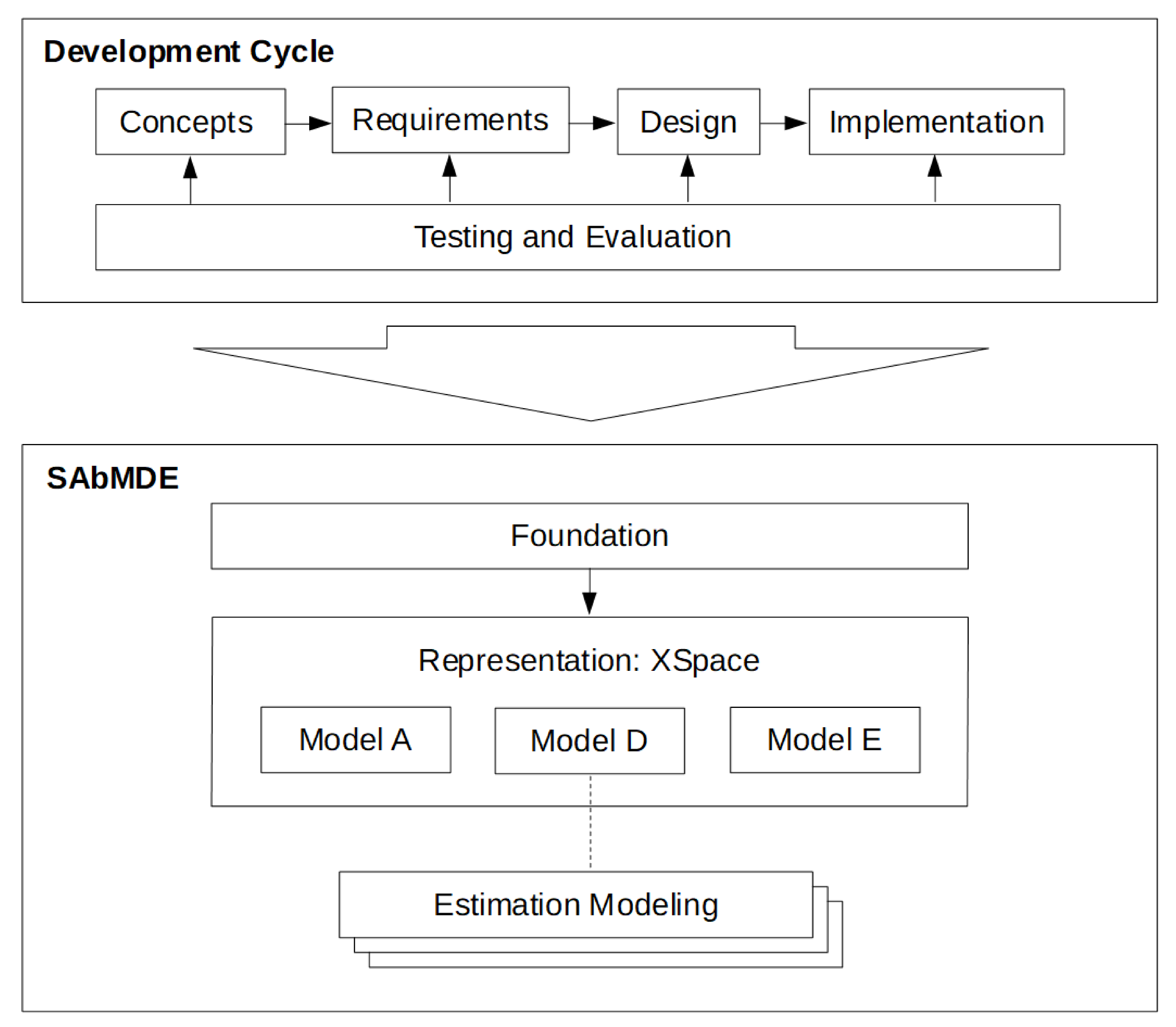
Figure 1. Development modeling framework.
Applsci 10 05013 g001
Figure 2. A simple development space (DSpace) excerpt with highlighted development paths (DPaths).
Applsci 10 05013 g002
Figure 3. Probability of sequential decision success.
Applsci 10 05013 g003
Figure 4. Cumulative resource utilization as estimated from each composition index (l).
Applsci 10 05013 g004
Figure 5. Cumulative resource utilization.
Applsci 10 05013 g005
Figure 6. Skill Indices for 16:1 estimate ratios by price.
Applsci 10 05013 g006
Figure 7. Constructive Cost Model (COCOMO) effort estimation for various program sizes measured in thousands of lines of source code (KLOC).
Applsci 10 05013 g007
Figure 8. Statistical Agent-based Model of Development and Evaluation (SAbMDE)-to-COCOMO effort estimation comparison for various KLOC values.
Applsci 10 05013 g008
Table 1. Hypergeometric retry count example.
nP(n)
10.99
20.98
30.97
880.12
890.11
900.10
910.09
920.08
Table 2. 16:1 Estimate Ratios by Skill Index.
Low Skill IndexHigh Skill Index
10.009.259.008.00
0.00111.00 38.5021.00
1.00111.00 38.5021.00
1.33 16.00
1.82 16.00
2.0031.0016.0011.006.00
Table 3. 16:1 Estimate Ratios by Backtrack Parameters.
Backtrack FactorBacktrack Length
123
0.0010.269.829.67
0.1010.189.789.64
0.2510.089.739.61
0.509.969.679.57
0.759.889.639.54
1.009.829.609.52
1.509.739.559.49
2.009.679.529.47
3.009.609.499.45
4.009.559.469.43
5.009.529.459.42
Table 4. COCOMO Scale Factors.
Scale FactorsScale Factor Range
Very LowLowNormalHighVery HighExtra High
PREC6.204.963.722.481.240.00
FLEX5.074.053.042.031.010.00
RESL7.075.654.242.831.410.00
TEAM5.484.383.292.191.100.00
PMAT7.806.244.683.121.560.00
Sum31.6225.2818.9712.656.320.00
Table 5. COCOMO Effort Multipliers.
Effort MultipliersEffort Multiplier Range
Very LowLowNormalHighVery High
ACAP1.421.191.000.850.71
PCAP1.341.151.000.880.08
PCON1.291.121.000.900.81
APEX1.221.101.000.880.81
PLEX1.191.091.000.910.85
LTEX1.201.091.000.910.84
Others1.001.001.001.001.00
Product4.282.001.000.490.03
Table 6. COCOMO Regression Parameters A–D.
NamesValues
KLOC100
A2.94
B0.91
C3.67
D0.28
Table 7. COCOMO Regression Parameters SF, EM, and E ranges.
NamesValues
Min(Effort)Max(Effort)
Effort Multipliers4.280.03
Scale Factors31.626.32
E1.230.97
Table 8. Skill Index and COCOMO Regression Parameter E, Adjusted.
StandardTruncatedAdjusted
COCOMOSAbMESAbMECOCOMO
Skill IndexScaled EMSkill IndexSkill IndexScaled EM
0.004.281.000.004.28
1.00
2.00
3.00
4.00
3.85
3.43
3.00
2.58
2.00
3.00
4.00
1.25
2.50
3.75
3.74
3.21
2.68
5.002.155.005.002.15
6.00
7.00
8.00
9.00
1.73
1.30
0.88
0.45
6.00
7.00
8.00
6.25
7.50
8.75
1.62
1.09
0.56
10.000.039.0010.000.03