Characterization of Inter-System Biases in GPS + BDS Precise Point Positioning

Abstract

With the combination of multi-GNSS data, the precise-point positioning (PPP) technique can improve its accuracy, availability and reliability: Inter-system bias (ISB) is the non-negligible parameter in multi-GNSS PPP. To further enhance the performance of multi-GNSS PPP, it is crucial to analyze the characterization of inter system biases (ISBs) and model them properly. In this contribution, we comprehensively investigate the characterization of ISBs between global positioning system (GPS) and BeiDou navigation satellite system (BDS) in different situations. (1) We estimate ISB by using different precise products from the Center for Orbit Determination (CODE), Deutsches GeoForschungsZentrum (GFZ) and Wuhan University (WHU). The results indicate that the one-day estimates of ISB are stable when using CODE and WHU products, whereas the estimates based on GFZ products vary remarkably. As for the three-day time series of ISB, a sudden jump exists between two adjacent days, which is due to the change of satellite clock datum; (2) We investigate the ISB characterization affected by the ambient environments of the receivers. The result shows that the ISBs estimated from receivers (and antennas) with same type are still inconsistent, which indicates that the ambient environment, probably the temperature, influences the ISB characterization as well, since the receivers are in different areas; (3) We analyze the ISB characterization affected by receiver and antenna type with the same ambient environment. To ensure the same ambient environment, the ultra-short baselines were applied to investigate the ISB characterization affected by the receiver and antenna type. With the insights into ISB characterizations, we carry out combined GPS and BDS PPP with modeling the ISB as time constant, random walk process and white noise. The results suggest that the random walk process outperforms in most cases, since it strengthens the model to some extend and, at the same time, considers the variation of ISBs.

1. Introduction

With the rapid developments and modernizations of the global navigation satellite systems (GNSSs) including the American GPS, Chinese BDS, European Galileo and Russian GLONASS, the integration of multi-GNSS brings a better and wider range of positioning, navigation, timing (PNT) and atmospheric retrieval applications [1,2,3,4,5,6]. As compared to GPS-only case, the multiple constellation increases the satellites in common view, thus enabling a higher accuracy and more reliability in precise-point positioning (PPP). The higher redundancy of the multi-GNSS model also shortens the initialization time of PPP. The combination of multi-GNSS opens up a new stage of its applications, whereas processing multi-GNSS data are more challenging [7,8].

The influence of intersystem bias (ISB) cannot be ignored in multi-GNSS PPP and unreasonable modeling of ISB will adversely affect the positioning accuracy and convergence speed [9]. In order to explore a reliable processing strategy of ISB, further investigation of its characteristic is necessary. After rigorous formula derivation, the ISB estimated by PPP contains the satellite clock datum and the receiver-code biases. Many agencies providing precise products have their own processing strategy in orbit determination and clock estimation, resulting in different satellite clock datums. Moreover, new efforts are made to rethink the assumption of constant receiver-code bias, which is closely related to temperature [10]. Therefore, to analyze the characterization of ISBs, a proper way is considering different satellite clock datums in precise products, the receiver (and antenna) type and other related factors such like the ambient environment (temperature) of the receiver.

Extensive studies have reported the influences of the abovementioned factors upon the ISB estimation. The receiver-code bias remarkably affects the ISB in the relative positioning [11,12]. The ISB between GPS and GLONASS is related to receiver type, antenna type and time system offset [13]. The code ISBs of BDS GEO, IGSO and MEO satellites to GPS estimated by single point positioning (SPP) are consistent [14]. The purpose of analyzing the characterization of ISBs is to model them more properly in PPP, many investigations provide their suggested strategies. A simple way is modeling the ISBs as constant process in one day [15,16,17,18], while some studies model the ISB as random walk process [19]. There also exist some investigations which model the ISB as white noise in the estimation [20]. In more detail, Zhou et al. believes that estimating ISBs as random walk or white noise process is much more reliable in multi-GNSS PPP processing [21]. Liu et al. find that the ISBs estimated with the center for orbit determination (CODE) and Wuhan University (WHU) final precise products are stable, which estimated with Deutsches GeoForschungsZentrum (GFZ) final precise products vary to a significant extent. Therefore, they recommends that, in GPS/BDS PPP, modeling the ISB as constant process when using precise products from the center for orbit determination (CODE) and Wuhan University (WHU) and modeling ISB as random walk when using precise products from Deutsches GeoForschungsZentrum (GFZ) [21]. In addition, some studies propose a short-term ISB model to predict the ISB in GPS/BDS-combined PPP [19].

To the best of our knowledge, there are few studies take the variation of the receiver-code bias into consideration. Whereas the receiver-code bias is affected by temperature and even exists a variation of ten meters. As we know, the ISB estimated by PPP contains the receiver-code bias. The question is how the variation of receiver-code bias influences the ISB. In this work, we further investigate the characterization of GPS/BDS ISBs in different scenarios. Except for estimating ISBs based on precise products from CODE, WHU and GFZ, we select the stations equipped with receivers of the same type in different areas to study whether or not the ambient environment (typically the temperature) of the receiver affects the ISB. Furthermore, the ultra-short baselines with the same ambient environment were applied to analyze the influence of receiver and antenna type in the ISB. After the analysis of ISB characterization, we implement combined GPS and BDS PPP with modeling the ISB as time constant, random walk process and white noise. The comparison of positioning performances will provide the guidance in proposing the optimal modeling strategy of ISB.

The remainder of this work is organized as follows: In the subsequent section, we review the undifferenced GPS/BDS PPP model and present the processing strategy. Following this, we designed four experiments to analyze, respectively, the influences of satellite clock datum, receiver type, antenna type and ambient environment upon ISB characterization. We also conducted a GPS/BDS PPP experiment with modeling ISB in different manners to find the optimal strategy. Finally, the last section presents summaries and conclusions.

2. Methods

This section reviews the full-rank undifferenced GPS/BDS model and gives insight into the estimable ISBs in the model. In addition, it also presents the processing strategy in detail.

The Undifferenced GPS/BDS PPP

Let us start with the original undifferenced observation equations. For a receiver-satellite combination $r-s$ at frequency $j$ in epoch $i$, the undifferenced code $P_{r,f}^{T,s}(i)$ and phase $L_{r,f}^{T,s}(i)$ observations are defined as [22]:

$$\begin{array}{l}{P}_{r,f}^{T,s}(i)={\rho }_r^{T,s}(i)+c\left(\Delta t_r^T(i)-\Delta t^{T,s}(i)\right)+{\mu }_f^T{I}_{r,1}^{T,s}(i)+T_r^s+b_{r,f}^T+b_f^{T,s}+{\epsilon }_P^T(i)\hfill \\ L_{r,f}^{T,s}(i)={\rho }_r^{T,s}(i)+c\left(\Delta t_r^T(i)-\Delta t^{T,s}(i)\right)-{\mu }_f^T{I}_{r,1}^{T,s}(i)+T_r^s+{\lambda }_f^T{N}_{r,f}^{T,s}+B_{r,f}^T+B_f^{T,s}+{\epsilon }_L^T(i)\hfill \end{array}$$

(1)

where superscript $T$ represents the system (G for GPS and C for BDS). ${\rho }_r^{T,s}(i)$ is the geometric distance; $c$ is the speed of light; $\Delta t_r^T(i)$ and $\Delta t^{T,s}(i)$ are the receiver and satellite clock offsets; $I_{r,1}^{T,s}(i)$ the (first-order) slant-ionosphere delay on the first frequency with its coefficient (${\mu }_f^T={\lambda }_f^2/{\lambda }_1^2$, in which ${\lambda }_f$ is the wavelength); $T_r^s$ is the tropospheric slant delay; $b_{r,f}^T$ and $b_f^{T,s}$ are the receiver and satellite code biases; $N_{r,f}^{T,s}$ is the integer ambiguity; $B_{r,f}^T$ and $B_f^{T,s}$ are receiver and satellite phase biases; ${\epsilon }_P(i)$ and ${\epsilon }_L(i)$ are noise in code and phase observation. Except $N_{r,f}^{T,s}$(unit: cycle), ${\lambda }_f$(unit: m/cycle) and ${\mu }_f^T$(without unit), all quantities are expressed in units of range.

Note that, the effects of phase windup, solid tide, ocean loading, relativistic effects, earth rotation have been corrected by corresponding models [23].

Conventionally, the IGS precise clock products absorb the ionosphere-free (IF) combination of satellite code biases as following [24]:

$$\widehat{\Delta }{t}^{T,s}(i)=\Delta t^{T,s}(i)-(\frac{{\mu }_2^T}{{\mu }_2^T-1}{b}_{r,1}^T-\frac{1}{{\mu }_2^T-1}{b}_{r,2}^T)$$

(2)

Equation (1) represents a rank-deficient system. In order to deal with the linear correlation between parameters (the receiver clock offsets with the receiver-code bias, the slant-ionosphere delay with the receiver-code bias, the ambiguities with the receiver and satellite phase biases, hardware biases between frequencies), the idea is to lump some of them together [25]. The reparameterization process is as below:

$$\begin{array}{l}{P}_f^{T,s}(i)={\rho }^{T,s}(i)+c\left[\Delta t_r^T(i)-\Delta t^{T,s}(i)\right]+{\mu }_f^T{I}_{r,1}^{T,s}(i)+T_r^s+b_{r,f}^T+b_f^{T,s}+{\epsilon }_P\\ ={\rho }^{T,s}(i)+c[\underset{\widehat{\Delta }{t}_r^T(i)}{\underbrace{\Delta t_r^T(i)+\frac{{\mu }_2^T}{{\mu }_2^T-1}{b}_{r,1}^T-\frac{1}{{\mu }_2^T-1}{b}_{r,2}^T}}-\widehat{\Delta }{t}^{T,s}(i)]\\ +\underset{{\mu }_f^T{\widehat{I}}_{r,1}^{T,s}(i)}{\underbrace{\frac{c{\mu }_f^T}{{\mu }_2^T-1}(b_{r,2}^T-b_{r,1}^T+b_2^{T,s}-b_1^{T,s})+{\mu }_f^T{I}_{r,1}^{T,s}(i)}}+T_r^s+{\epsilon }_P(i)\end{array}$$

(3)

$$\begin{array}{l}{L}_f^{T,s}(i)={\rho }^{T,s}(i)+c[\widehat{\Delta }{t}_r^T(i)-\widehat{\Delta }{t}^{T,s}(i)]+{\mu }_f^T{\widehat{I}}_{r,1}^{T,s}(i)+T_r^s+\\ {\lambda }_f^T\left\{\underset{{\widehat{N}}_{r,f}^{T,s}}{\underbrace{N_{r,f}^{T,s}+B_{r,f}^T+B_f^{T,s}+\frac{c}{{\lambda }_f^T({\mu }_2^T-1)}[({\mu }_f^T+1)(b_{r,2}^T+b_2^{T,s})-({\mu }_f^T+{\mu }_2^{T,s})(b_{r,1}^T+b_1^{T,s})]}}\right\}+{\epsilon }_L\end{array}$$

(4)

where ^ presents that the parameter after recombination. The full-rank GPS/BDS PPP observation equations can be rewritten as

$$\begin{array}{l}{P}_f^{T,s}(i)={\rho }^{T,s}(i)+c[\widehat{\Delta }{t}_r^T(i)-\widehat{\Delta }{t}^{T,s}(i)]+{\mu }_f^T{\widehat{I}}_{r,1}^{T,s}(i)+T_r^s+{\epsilon }_P(i)\hfill \\ L_f^{T,s}(i)={\rho }^{T,s}(i)+c[\widehat{\Delta }{t}_r^T(i)-\widehat{\Delta }{t}^{T,s}(i)]-{\mu }_f^T{\widehat{I}}_{r,1}^{T,s}(i)+T_r^s+{\lambda }_f^T{\widehat{N}}_f^{T,s}+{\epsilon }_L(i)\hfill \end{array}$$

(5)

We select the estimable GPS receiver clock $\widehat{\Delta }{t}_r^G$ as reference, then the GPS/BDS ISB can be denote as

$$\begin{array}{l}IS{B}^{G,C}=\widehat{\Delta }{t}_r^C-\widehat{\Delta }{t}_r^G\\ =(\overline{\Delta }{t}_r^C-\overline{\Delta }{t}_r^G)+(\frac{{\mu }_2^C}{{\mu }_2^C-1}{b}_{r,1}^C-\frac{1}{{\mu }_2^C-1}{b}_{r,2}^C)-(\frac{{\mu }_2^G}{{\mu }_2^G-1}{b}_{r,1}^G-\frac{1}{{\mu }_2^G-1}{b}_{r,2}^G)\\ =(\Delta t_r^C-\Delta t_r^G)+(\Delta D^G-\Delta D^C)+(\frac{{\mu }_2^C}{{\mu }_2^C-1}{b}_{r,1}^C-\frac{1}{{\mu }_2^C-1}{b}_{r,2}^C)-(\frac{{\mu }_2^G}{{\mu }_2^G-1}{b}_{r,1}^G-\frac{1}{{\mu }_2^G-1}{b}_{r,2}^G)\end{array}$$

(6)

where $\overline{\Delta }{t}_r^G$ and $\overline{\Delta }{t}_r^C$ respectively represent the GPS and BDS receiver clock offset which absorb the satellite clock datum. $\Delta D^G$ and $\Delta D^C$ are GPS and BDS satellite clock datum, respectively. For the reason that the receiver and satellite clock parameters are linear dependent, a reference of clock offset must be set for each system [26]. In the meantime, the variation of the reference will be absorbed in the receiver clock offset. Therefore, the ISB obtained by PPP contains the offsets of inter-system satellite clock datums and the receiver-code biases.

The state vector X of GPS/BDS undifferenced and uncombined PPP can be written as

$$X=[\begin{array}{lllllll}x\hfill & \widehat{\Delta }{t}_r^G(i)\hfill & T_r^s\hfill & {\widehat{I}}_{r,1}^{G,s}(i)\hfill & {\widehat{I}}_{r,1}^{C,s}(i)\hfill & {\widehat{N}}_{r,f}^{G,s}\hfill & {\widehat{N}}_{r,f}^{C,s}\hfill \end{array}]$$

(7)

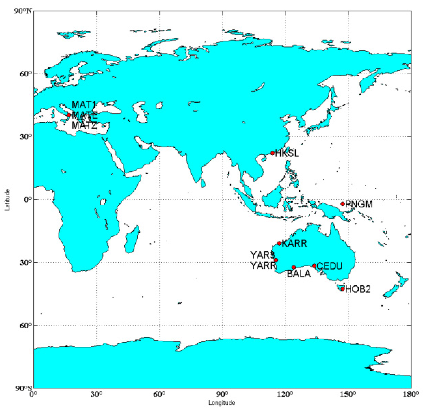
3. Processing Strategy

The final precise orbit (5 min interval for CODE and GFZ, 15 min interval for WHU) and clock products (30 s interval) from Wuhan University (WUM), center for orbit determination (CODE) and Deutsches GeoForschungsZentrum (GFZ) were employed. The absolute antenna phase-center correction models (igs14.atx) were applied to correct the phase-center offset and variation, which for BDS satellites obtained from European Space Agency (ESA). In order to analyze the characteristics of ISB, the ISB is modeled as white noise. The UNB3 model was used to correct the tropospheric dry delay and the tropospheric zenith wet delay is estimated as parameter, with Neil as the mapping function. The float phase ambiguities were estimated as constant for each continuous satellite arc. The traditional methods—turbo-edit detection—namely the geometry-free and MW observations were applied in the detection of cycle slip [27]. The elevation cutoff angle was set to $7°$ and an elevation-dependent weighting scheme (${\sin }^2(elevation)$) for the observation was applied [28]. The weight ratio of GPS and BDS is set at 1:1.5 [29]. Due to the BDS GEO satellite orbit and clock accuracy, the weight of BDS GEO satellite observations is reduced by 10 times [30]. In order to strengthen the model, we estimated the ISBs with static PPP processing. The detail processing strategies are shown in

Table 1. Adopted models and strategies.

Options	Processing Strategies
System	GPS/BDS
Observation interval	30 s
Estimation principal	Kalman filter
Frequency	L1,L2/B1,B2
Elevation cutoff angle	7°
Receiver clock	White noise
Inter-system bias (ISB)	White noise
Ionospheric delay	White noise
Tropospheric delay	Random walk $({10}^{-8}{\mathrm{m}}^2/\mathrm{s})$
Receiver coordinates	Static
Ambiguities	Constant over time

. The distribution of the selected stations is shown in Figure 1.

4. Characterization of ISB

According to Equation (6), the ISB estimated by PPP contains the satellite clock datum and the receiver-code bias. In the following, undifferenced and uncombined PPP was adopted to analyze the influence factors of ISB. The technical features of the receiver and antenna types mentioned in the experiments are available in the official websites, TRIMBLE (https://geospatial.trimble.com), LEICA (https://leica-geosystems.com), SETPENTRIO (https://www.septentrio.com).

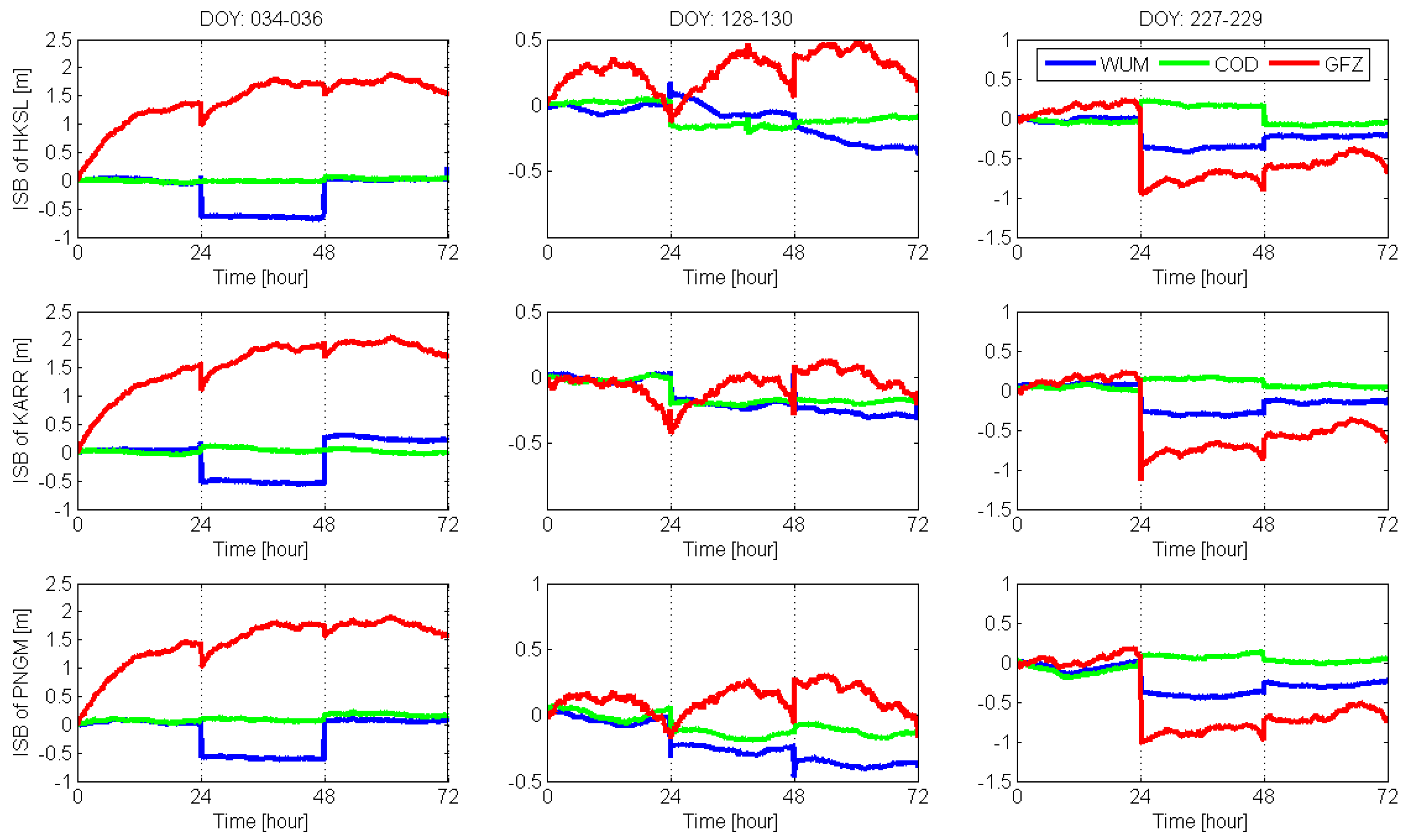
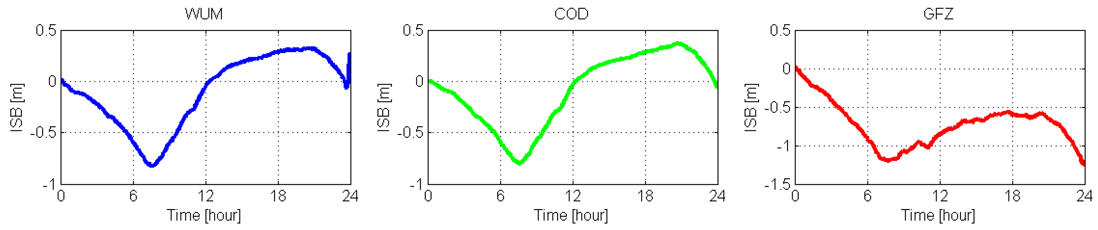
4.1. ISB Characterization Affected by the Satellite Clock Datum

In this experiment, randomly, we collect data from three IGS stations including PNGM, HKSL and GAMG from day of year (DOY) 034–036, day of year (DOY) 128–130, day of year (DOY) 227–229, 2018, respectively. The observation data are available over FTP (ftp://cddis.gsfc.nasa.gov) for free.

The absolute ISBs estimated with different precise products differ a lot in magnitude. To show the results clearly, all estimates are subtracted by the ISB estimated in first epoch.

Figure 2 shows the ISB time series of three stations using WUH, CODE and GFZ precise products, respectively. The ISBs suddenly jump between two adjacent days, and the amplitude of the fluctuation is different-with-different precise products. This fluctuation is caused by the change of satellite clock datum [31]. Moreover, the daily ISBs based on CODE and WHU products are stable, while the variation of daily ISBs corresponding to GFZ products is remarkable. As we can see, the time series of ISBs from three stations using same products are consistent. It further proves that the change of satellite clock datum affects the ISBs.

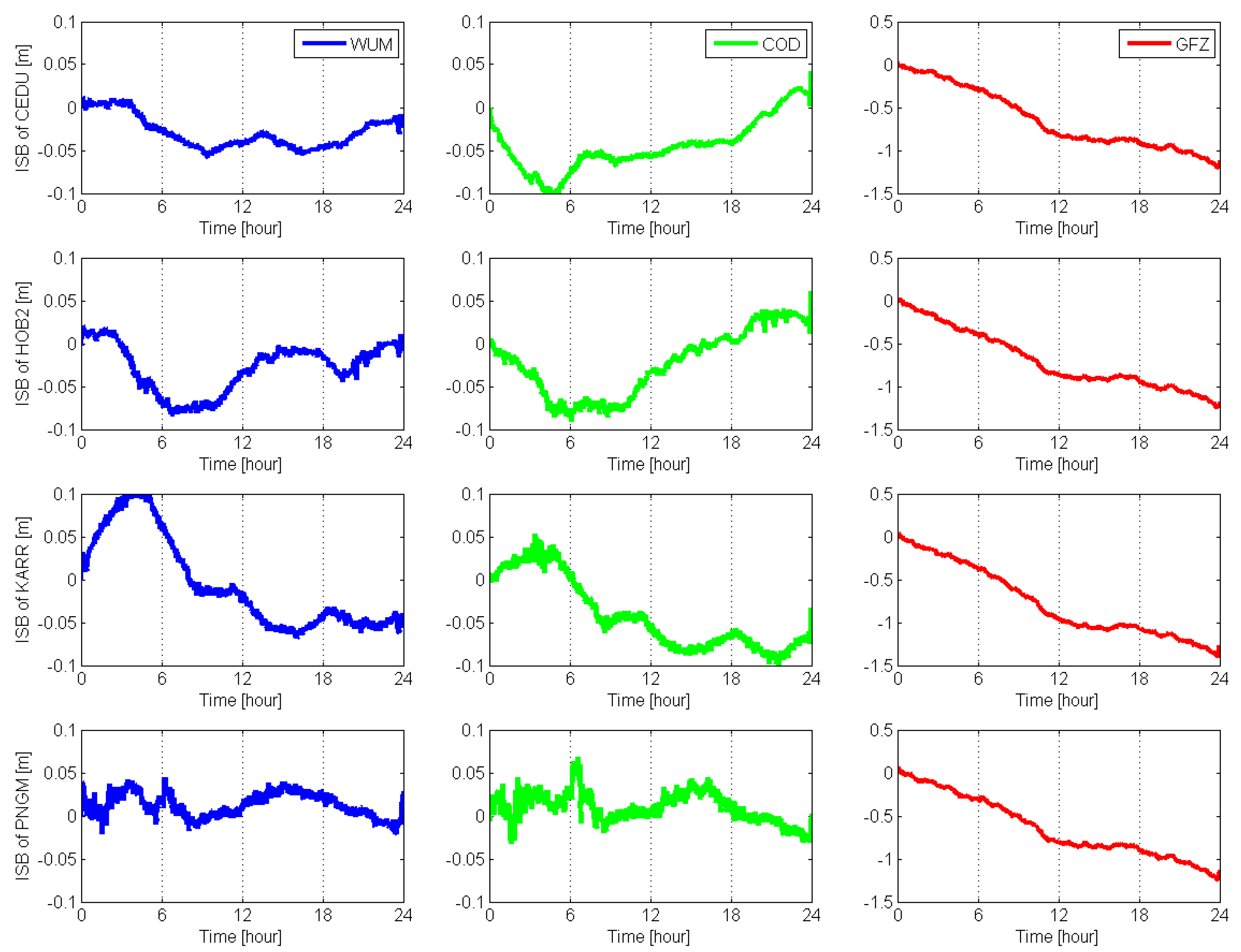
4.2. ISB Characterization Affected by the Ambient Environment

Four IGS stations (CEDU HOB2 KARR and PNGM) are selected on DOY 002, 2018. Stations CEDU and HOB2 are equipped with SEPT POLARX5 receivers while stations KARR and PNGM are equipped with TRIMBLE NETR9 receivers. For more detailed information, see

Table 2. Stations selected for the investigation of ISB characterization affected by the ambient environment.

Station	Receiver type	Antenna type
CEDU	SEPT POLARX5	AOAD/M_T
HOB2	SEPT POLARX5	AOAD/M_T
KARR	TRIMBLE NETR9	TRM59800.00
PNGM	TRIMBLE NETR9	TRM59800.00

.

Figure 3 shows that the ISBs estimated with the WUM and CODE precise products showed little fluctuation. It is worth noting that even though stations KARR and PNGM were equipped with the same type of receivers and antennas, the ISB estimate were still different when using WUM and CODE precise products. We surmised that the ambient environment of the receiver, probably the temperature, may have affected the characterization of ISBs [10]. However, for the reason that the satellite clock datum of GFZ final products vary over time significantly, the difference between the different stations could not perform notably.

4.3. Discussion

Figure 3 shows that the ISBs obtained with even the same receiver and antenna type, they had little difference. Therefore, in order to investigate the receiver and antenna type affected the ISB characterization, we collected the data from ultra-short baseline (about several meters) stations to ensure the same ambient environments. We discuss the implication of receiver and antenna type in more detail below.

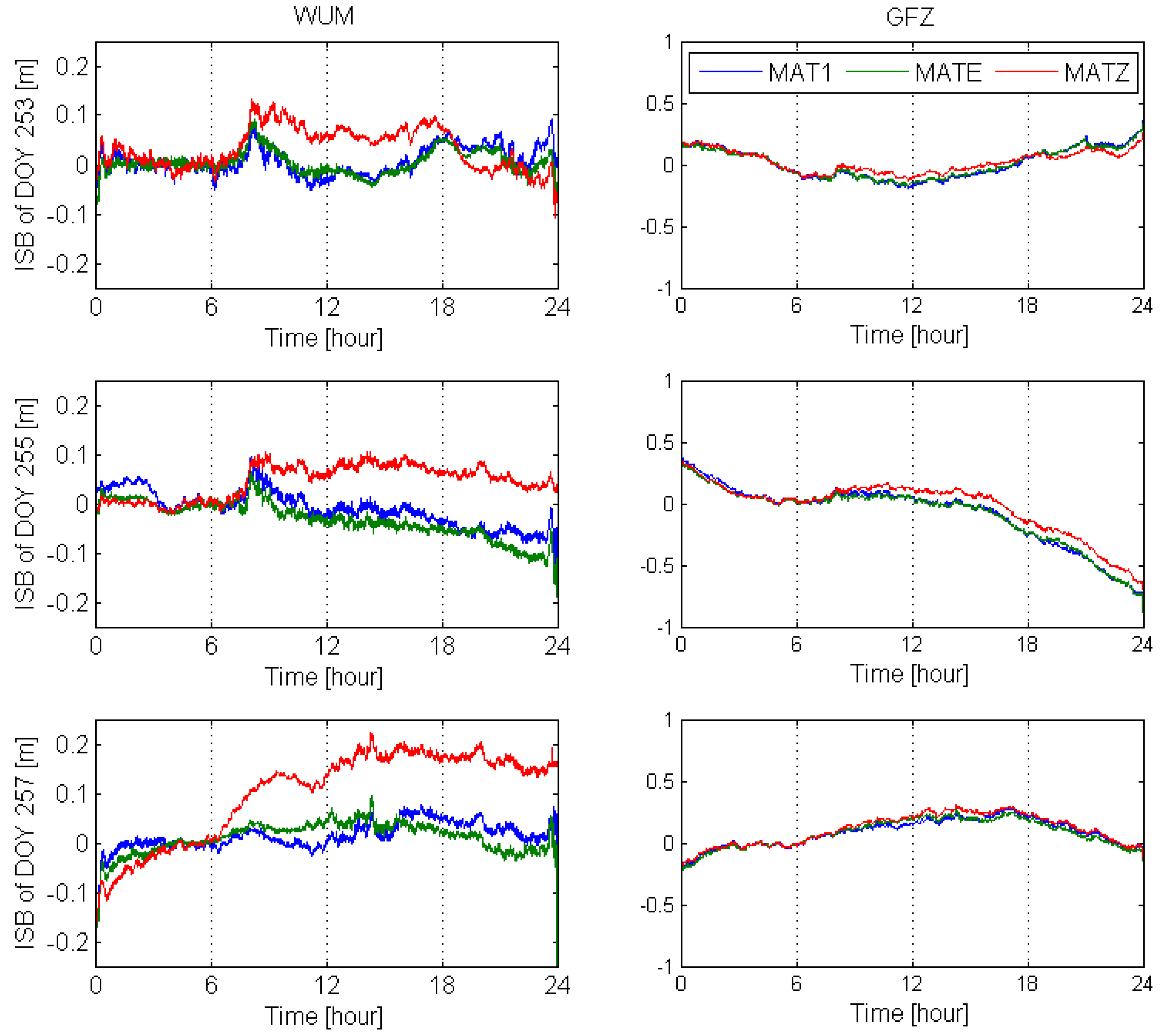
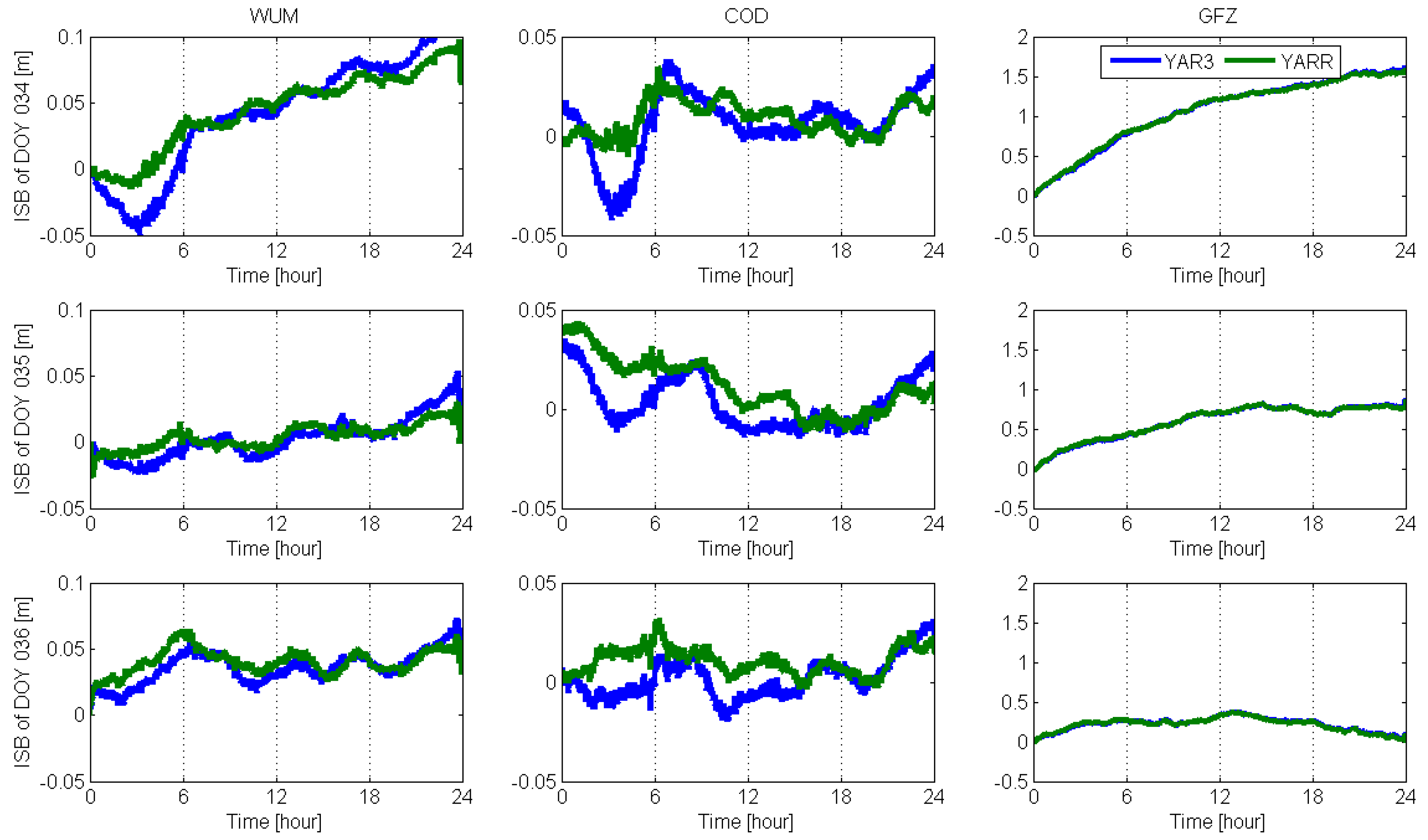
4.4. ISB Characterization Affected by the Receiver Type

As shown in

Table 3. Stations selected for the investigation of ISB characterization affected by the receiver type.

Station	Receiver Type	Antenna Type
MAT1	LEICA GR30	LEIAR20
MATE	LEICA GR30	LEIAR20
MATZ	SEPT POLARX5TR	LEIAR20

, this experiment selects two stations (MAT1, MATE) equipped LEICA GR30 receivers and one station equipped SEPT POLARX5TR receiver. All of them were connected to LEIAR20 antennas. The distance between any two of them was less than 30 m. Therefore, we assumed that the external temperature of three stations was identical. For the reason that the observed BDS satellites were not enough, we only estimated the ISBs using WUM and GFZ products in this experiment due to the CODE precise products exclude the BDS GEO satellites. For the same reason, we skipped the data on DOY 254 and 256, 2018 and displayed the results on DOY 253, 255 and 257, 2018.

Figure 4 shows the ISB estimated from station MAT1, MAE1 and MAZ1. We see that the ISB time series from stations MAT1 and MATE equipped receivers with same type were consistent. However, see the results from station MATZ, which was equipped with the other type of receiver, the ISB estimates differed from the results from stations MAT1 and MAE1 in some periods. Typically, in the period of hour after 8, there was an offset about 0.1 m between ISBs from two types of receivers when using WUM products. As we can see, the gaps of ISB estimated by different receiver types were similar, it due to the variation of the receiver-code bias was closely related to temperature [10], while the temperatures were comparable in the adjacent days. In addition, the ISBs based on WUM products were more stable than those based on GFZ products, which was in accordance with what we find in Figure 2.

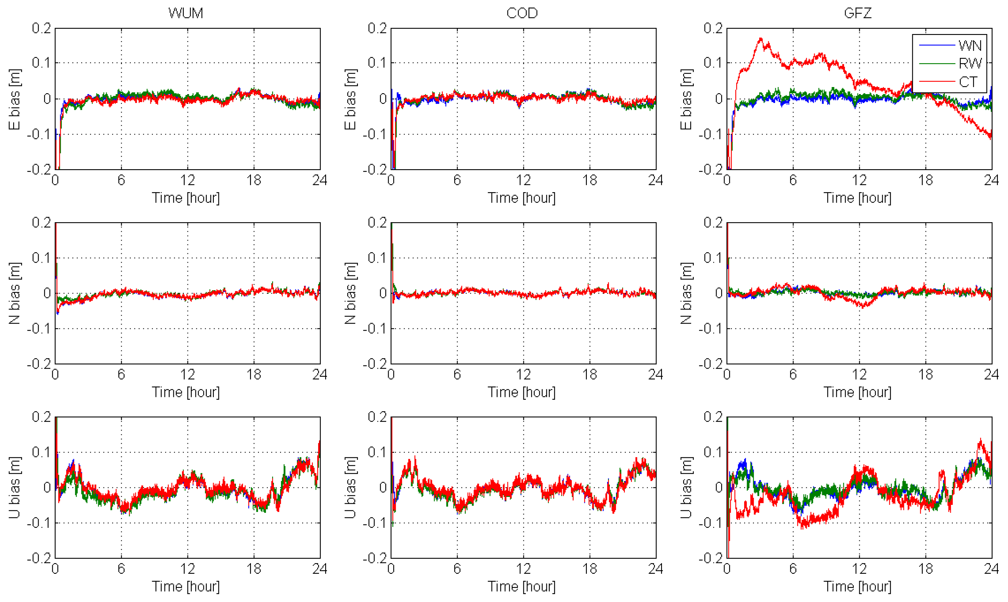
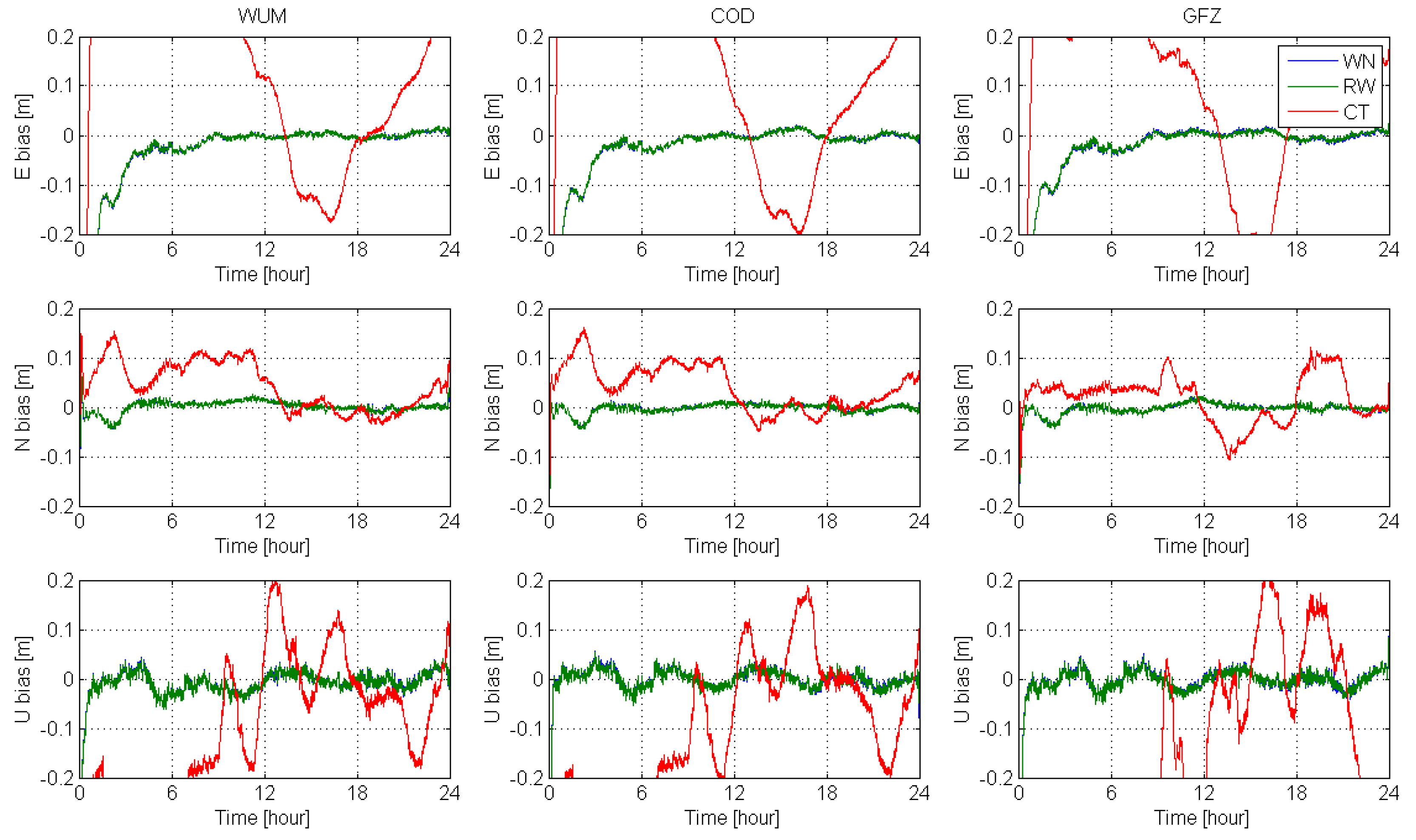
4.5. ISB Characterization Affected by the Antenna Type

This experiment aimed to find out whether the ISB characterization was related to antenna type or not. See

Table 4. Stations selected for the investigation of ISB characterization affected by the antenna type.

Station	Receiver Type	Antenna Type
YARR	SEPT POLARX5	LEIAT504
YAR3	SEPT POLARX5	LEIAR25

, we select stations YARR and YAR3 equipped with the SEPT PLOARX5 receivers. Station YARR was connected to LEIAT504 antenna, while was YAR3 connected to LEIAR25 antenna. Similar as before, the distance between YARR and YAR3 was less than 30 m, the external temperature of these two stations could be considered very similar.

Figure 5 shows, the ISBs from different antennas were inconsistent when using WUM and CODE products, due to the smaller scales, the differences of ISB estimated with CODE precise products were more significant. This indicate that the ISB was related to antenna type and it may be caused by antenna and cable induced delay [32], thus making the ISB antenna-specific. However, the ISBs based on GFZ products were consistent, this was because the ISB variation caused by the change of satellite clock datum were much larger than the variation caused by the antenna code bias.

Based on the analysis of ISB characterizations, we carried out the GPS/BDS PPP with modeling the ISB as, constant (CT), random walk (RW) process and white noise (WN) [33], respectively. Data from twelve IGS stations on DOY 252–281, 2018 were used to analyze the performances of GPS/BDS float dynamic PPP using different ISB modeling strategies. Taking station PNGM as an example randomly, the GPS/BDS float dynamic PPP solutions were carried out with modeling ISB as constant, random walk and white noise process. As for the equipped receivers and antennas, refer to Table 2.

Figure 6 shows that, for the PNGM station, the positioning errors in east, north and up were almost the same with different modeling strategies of ISB using WUM and CODE precise products, while the solution using GFZ precise products, the performance with constant ISB modeling strategies were much worse than random walk and white noise ISB modeling strategies. Taken altogether, as

Table 5. RMS (cm) of GPS/BDS PPP result among different ISB modeling with different precise products.

	Constant			Random Walk			White Noise
	Horizontal	Vertical	3D	Horizontal	Vertical	3D	Horizontal	Vertical	3D
WUM	2.25	3.90	4.50	2.52	4.06	4.48	2.70	4.24	5.03
COD	2.02	3.68	4.20	2.29	3.84	4.45	2.46	3.91	4.62
GFZ	8.66	9.71	13.2	2.34	3.82	4.48	2.36	3.87	4.53

and

Table 6. Average times (minutes) of GPS/BDS PPP result convergence to 10 cm in horizontal and vertical directions and maintained for one hour among different ISB handling methods with different precise products.

	Constant		Random Walk		White Noise
	Horizontal	Vertical	Horizontal	Vertical	Horizontal	Vertical
WUM	39.4	26.5	42.1	27.7	45.2	30.0
COD	37.5	25.3	40.4	25.9	44.7	29.2
GFZ	157.3	31.1	47.7	26.6	46.9	29.8

, similar to the positioning performance, the convergence performances were almost uniform with different modeling strategies of ISB, the performances of GPS/BDS PPP based on CODE and WUM products were comparable. In these three cases, the CT process performs best, the RW process follows, and the WN process presents the worst performance. This was confirmed with the stability of ISBs based on CODE and WUM precise products. As for the results based on GFZ precise products, estimate the ISB as constant is not reasonable because it always performs great variation. Therefore, the results using RW and WN processing strategies were comparable, which were better than the results using CT processing strategy.

Consistently, the receiver-code biases from all the multi-GNSS experiment (MGEX) tracking stations demonstrate consistent stability as those from the stations we selected. Therefore, according to Table 5 and Figure 6, we came up with the results consistent with previous studies. However, the receiver-code bias was not always stable.

Peculiarly, we found that some stations varied significantly in receiver-code bias. Take the data from BALA on DAY 002, 2018 for example (besides GASC, JLCK, LAMB, MTDN, UCAL, etc. having the similar performance). This is freely available at Geoscience Australia FTP (ftp://ftp.ga.gov.au/). The station BALA is equipped with TRIMBLE NETR9 receiver and LEIAR25.R3 antenna.

As Figure 7 shown, the ISBs estimated by using CODE and WUM precise products were not always that stable due to the variation of receiver-code bias. Wrongly estimated the ISB as constant would carry out a terrible positioning performance as Figure 8. Therefore, we suggest that estimating ISB as random walk or white noise was more reliable, instead of constant.

5. Summary and Conclusions

In this contribution, we comprehensively analyzed the characterization of inter-system biases (ISBs) with different precise products, receiver types and antenna types. We also investigated whether or not the ambient environment of the receiver affects the ISB characterization. Based on the analysis of ISB characterization, we implemented the GPS/BDS PPP with modeling the ISB as time constant, random walk process and white noise.

A sudden jump exists in the ISB estimates between two adjacent days. It is caused by the change of satellite clock datum. The ISBs estimated with the precise products from different analysis centers have significant divergence. It is found that, in most cases, the estimated ISBs using WUM and CODE products are stable, while the variation of ISBs estimated by using GFZ products is remarkable. This is determined by the data processing strategies adopted in by different analysis centers. Moreover, even the stations equipped with the same type of receivers and antennas, the ISBs are inconsistent. This is because the stations are located in different places where the ambient environments (e.g., temperature) are different and the receiver-code biases are closely related to the temperature. The data from ultra-short baselines are used to confirm the same ambient environment, the result indicate that the receiver and antenna type both affects the characterization of ISBs. Therefore, besides the impact of different final precise products, the receiver type, antenna type and even the ambient environment affect the ISB characterizations.

For GPS/BDS PPP solutions with WUM and CODE precise products, the positioning performances agree well among the three ISB processing methods. However, when the receiver-code biases vary significantly and GFZ precise products are used, the results of GPS/BDS PPP obtained by random walk or white noise are more accurate than those using the constant method.

References

1. Defraigne, P.; Baire, Q. Combining GPS and GLONASS for time and frequency transfer. Adv. Space Res. 2011, 47, 265–275. [Google Scholar] [CrossRef]
2. Gao, Z.; Zhang, H.; Ge, M.; Niu, X.; Shen, W.; Wickert, J.; Schuh, H. Tightly coupled integration of multi-GNSS PPP and MEMS inertial measurement unit data. GPS Solut. 2017, 21, 377–391. [Google Scholar] [CrossRef]
3. Li, W.; Wang, G.; Mi, J.; Zhang, S. Calibration errors in determining slant Total Electron Content (TEC) from multi-GNSS data. Adv. Space Res. 2019, 63, 1670–1680. [Google Scholar] [CrossRef]
4. Yuan, Y.; Wang, N.; Li, Z.; Huo, X. The BeiDou global broadcast ionospheric delay correction model (BDGIM) and its preliminary performance evaluation results. Annu. Navig. 2019, 66, 55–69. [Google Scholar] [CrossRef] [Green Version]
5. Zhang, B.; Chen, Y.; Yuan, Y. PPP-RTK based on undifferenced and uncombined observations: Theoretical and practical aspects. J. Geod. 2019, 93, 1011–1024. [Google Scholar] [CrossRef]
6. Zhang, B.; Teunissen, P.J.G.; Odijk, D. A novel un-differenced PPP-RTK concept. J. Navig. 2011, 64, S180–S191. [Google Scholar] [CrossRef] [Green Version]
7. Cai, C.; Gao, Y.; Pan, L.; Zhu, J. Precise point positioning with quad-constellations: GPS, BeiDou, GLONASS and Galileo. Adv. Space Res. 2015, 56, 133–143. [Google Scholar] [CrossRef]
8. Li, X.; Zhang, X.; Ren, X.; Fritsche, M.; Wickert, J.; Schuh, H. Precise positioning with current multi-constellation Global Navigation Satellite Systems: GPS, GLONASS, Galileo and BeiDou. Sci. Rep. 2015, 5, 8328. [Google Scholar] [CrossRef] [PubMed]
9. Zhou, F.; Dong, D.; Li, P.; Li, X.; Schuh, H. Influence of stochastic modeling for inter-system biases on multi-GNSS undifferenced and uncombined precise point positioning. GPS Solut. 2019, 23, 59. [Google Scholar] [CrossRef]
10. Zha, J.; Zhang, B.; Yuan, Y.; Zhang, X.; Li, M. Use of modified carrier-to-code leveling to analyze temperature dependence of multi-GNSS receiver DCB and to retrieve ionospheric TEC. GPS Solut. 2019, 23, 103. [Google Scholar] [CrossRef]
11. Odijk, D.; Teunissen, P.J. Characterization of between-receiver GPS-Galileo inter-system biases and their effect on mixed ambiguity resolution. GPS Solut. 2013, 17, 521–533. [Google Scholar] [CrossRef]
12. Dalla Torre, A.; Caporali, A. An analysis of intersystem biases for multi-GNSS positioning. GPS Solut. 2015, 19, 297–307. [Google Scholar] [CrossRef]
13. Chen, J.; Xiao, P.; Zhang, Y.; Wu, B. GPS/GLONASS system bias estimation and application in GPS/GLONASS combined positioning. In Proceedings of the China satellite Navigation Conference (CSNC) 2013, Wuhan, China, 15–17 May 2013; pp. 323–333. [Google Scholar]
14. Zeng, A.; Yang, Y.; Ming, F.; Jing, Y. BDS–GPS inter-system bias of code observation and its preliminary analysis. GPS Solut. 2017, 21, 1573–1581. [Google Scholar] [CrossRef]
15. Guo, J.; Li, X.; Li, Z.; Hu, L.; Yang, G.; Zhao, C.; Fairbairn, D.; Watson, D.; Ge, M. Multi-GNSS precise point positioning for precision agriculture. Precis. Agric. 2018, 19, 895–911. [Google Scholar] [CrossRef] [Green Version]
16. Li, X.; Ge, M.; Dai, X.; Ren, X.; Fritsche, M.; Wickert, J.; Schuh, H. Accuracy and reliability of multi-GNSS real-time precise positioning: GPS, GLONASS, BeiDou, and Galileo. J. Geod. 2015, 89, 607–635. [Google Scholar] [CrossRef]
17. Liu, T.; Yuan, Y.; Zhang, B.; Wang, N.; Tan, B.; Chen, Y. Multi-GNSS precise point positioning (MGPPP) using raw observations. J. Geod. 2017, 91, 253–268. [Google Scholar] [CrossRef]
18. de Bakker, P.F.; Tiberius, C.C. Real-time multi-GNSS single-frequency precise point positioning. GPS Solut. 2017, 21, 1791–1803. [Google Scholar] [CrossRef] [Green Version]
19. Jiang, N.; Xu, Y.; Xu, T.; Xu, G.; Sun, Z.; Schuh, H. GPS/BDS short-term ISB modelling and prediction. GPS Solut. 2017, 21, 163–175. [Google Scholar] [CrossRef] [Green Version]
20. Hong, J.; Tu, R.; Gao, Y.; Zhang, R.; Fan, L.; Zhang, P.; Liu, J. Characteristics of inter-system biases in Multi-GNSS with precise point positioning. Adv. Space Res. 2019, 63, 3777–3794. [Google Scholar] [CrossRef]
21. Liu, X.; Jiang, W.; Chen, H.; Zhao, W.; Huo, L.; Huang, L.; Chen, Q. An analysis of inter-system biases in BDS/GPS precise point positioning. GPS Solut. 2019, 23, 116. [Google Scholar] [CrossRef]
22. Leick, A.; Rapoport, L.; Tatarnikov, D. GPS Satellite Surveying; John Wiley & Sons: Hoboken, NJ, USA, 2015. [Google Scholar]
23. Kouba, J. A Guide to Using International GNSS Service (IGS) Products; Kouba, Jan: Pasadena, CA, USA, 2009. [Google Scholar]
24. Kouba, J.; Héroux, P. Precise point positioning using IGS orbit and clock products. GPS Solut. 2001, 5, 12–28. [Google Scholar] [CrossRef]
25. Odijk, D.; Zhang, B.; Khodabandeh, A.; Odolinski, R.; Teunissen, P.J.G. On the estimability of parameters in undifferenced, uncombined GNSS network and PPP-RTK user models by means of \mathcal {S}-system theory. J. Geod. 2016, 90, 15–44. [Google Scholar] [CrossRef]
26. Han, S.; Kwon, J.H.; Jekeli, C. Accurate absolute GPS positioning through satellite clock error estimation. J. Geod. 2001, 75, 33–43. [Google Scholar] [CrossRef]
27. Blewitt, G. An automatic editing algorithm for GPS data. Geophys. Res. Lett. 1990, 17, 199–202. [Google Scholar] [CrossRef] [Green Version]
28. Wang, J.; Stewart, M.; Tsakiri, M. Adaptive Kalman filtering for integration of GPS with GLONASS and INS. In Geodesy beyond 2000; Presentation at the XXIIth International Union for Geodesy and Geophysics (IUGG); Springer: Berlin/Heidelberg, Germany, 2000; pp. 325–330. [Google Scholar]
29. Hou, P.; Zhang, B.; Yuan, Y. Analysis of the stochastic characteristics of GPS/BDS/Galileo multi-frequency observables with different types of receivers. J. Spat. Sci. 2019, 1–25. [Google Scholar] [CrossRef]
30. Pan, L.; Xiaohong, Z.; Fei, G. Ambiguity resolved precise point positioning with GPS and BeiDou. J. Geod. 2017, 91, 25–40. [Google Scholar] [CrossRef]
31. Zhang, H.; Hao, J.; Liu, W.; Yu, H.; Tian, Y. A Kalman filter method for BDS/GPS short-term ISB modelling and prediction. Acta Geod. Cartogr. Sin 2016, 45, 31–38. [Google Scholar]
32. Tegedor, J.; Øvstedal, O.; Vigen, E. Precise orbit determination and point positioning using GPS, Glonass, Galileo and BeiDou. J. Geod. Sci. 2014, 4, 65–73. [Google Scholar] [CrossRef] [Green Version]
33. Grewal, M.S.; Andrews, A.P. Kalman Filtering: Theory and Practice with MATLAB; John Wiley & Sons: New York, NY, USA, 2014. [Google Scholar]
Figure 1. Geographic distribution of stations used in the global positioning system (GPS)/ BeiDou navigation satellite system (BDS) precise-point positioning (PPP) experiment to analyze the characteristic of inter-system bias (ISB).
Applsci 10 04968 g001
Figure 2. GPS/BDS ISB series from stations HKSL, KARR and PNGM stations estimated by using Wuhan University (WHU), Center for Orbit Determination (CODE) and Deutsches GeoForschungsZentrum (GFZ) precise products during DOY 043–036, 128–130 and 227–229, 2018.
Applsci 10 04968 g002
Figure 3. GPS/BDS ISB series of CEDU/HOB2/KARR and PNGM stations estimated using WHU, CODE and GFZ precise products on DOY 002, 2018.
Applsci 10 04968 g003
Figure 4. GPS/BDS ISB series of MAT1/MATE and MATZ estimated using WHU, CODE and GFZ precise products on DOY 253, 255, 257, 2018.
Applsci 10 04968 g004
Figure 5. GPS/BDS ISB series of YARR and YAR3 stations estimated using WHU, CODE and GFZ precise products on DOY 034–036, 2018.
Applsci 10 04968 g005
Figure 6. Positioning result of GPS/BDS PPP at station PNGM on DOY 252, 2018, using constant, random walk and white noise methods.
Applsci 10 04968 g006
Figure 7. GPS/BDS ISB series of BALA WHU, CODE and GFZ precise products on DOY 002, 2018.
Applsci 10 04968 g007
Figure 8. Positioning result of GPS/BDS PPP at station BALA on DOY 2, 2018, using constant, random walk and white noise methods.
Applsci 10 04968 g008