Airflow Characteristics Downwind a Naturally Ventilated Pig Building with a Roofed Outdoor Exercise Yard and Implications on Pollutant Distribution

Abstract

The application of naturally ventilated pig buildings (NVPBs) with outdoor exercise yards is on the rise mainly due to animal welfare considerations, while the issue of emissions from the buildings to the surrounding environment is important. Since air pollutants are mainly transported by airflow, the knowledge on the airflow characteristics downwind the building is required. The objective of this research was to investigate airflow properties downwind of a NVPB with a roofed outdoor exercise yard for roof slopes of 5°, 15°, and 25°. Air velocities downwind a 1:50 scaled NVPB model were measured using a Laser Doppler Anemometer in a large boundary layer wind tunnel. A region with reduced mean air velocities was found along the downwind side of the building with a distance up to 0.5 m (i.e., 3.8 times building height), in which the emission concentration might be high. Additional air pollutant treatment technologies applied in this region might contribute to emission mitigation effectively. Furthermore, a wake zone with air recirculation was observed in this area. A smaller roof slope (i.e., 5° slope) resulted in a higher and shorter wake zone and thus a shorter air pollutant dispersion distance.

1. Introduction

Natural ventilation systems have the advantages of low capital investment, energy saving [1], and absence of noise [2] compared with mechanical ventilation systems. Thus, they are widely implemented in livestock buildings. Naturally ventilated pig production systems equipped with outdoor exercise yards are receiving increasing interest in Europe, the United States, and South Africa [3,4]. This housing system provides pigs larger living areas, enables the separation of lying and excretion areas, and allows pigs to exhibit natural behaviours [5]. It provides pigs access to an outdoor exercise area, enables pigs to mainly excrete outdoors, and thus results in improved indoor air quality [6], animal welfare [3], and meat quality [7] compared with a conventional housing system. The design of naturally ventilated pig buildings (NVPBs) with outdoor access is mainly based on the consideration of animal production performance and animal welfare [3,8].

However, one important issue associated with this type of buildings is the amount of air pollutants produced in the buildings and their emission to the surrounding environment. The open-type barn structure allows a direct air exchange between the indoor and outdoor environment, and consequently leads to a wide dispersion of gaseous emissions into the atmosphere [9]. The gaseous pollutants produced from the buildings including ammonia, greenhouse gases, hydrogen sulphide, particulate matter, odours and aerosols contribute to environmental problems and causes nuisance to neighbouring residents [10]. The transport and dispersion processes of gaseous emissions are strongly affected by airflow [11,12], which is influenced by the atmospheric boundary layer (ABL) such as temperature, humidity, wind speed, wind direction, and terrain [13]. The ABL experiences periodic evolution of daytime convective [14], transitional (occurs in the morning, late afternoon or early evening) [15], and nocturnal stable states [16] due to the solar diurnal cycle. This dynamic behaviour of the ABL may also affect the evolution of particulate matter [17]. In addition to the ABL, building configurations (e.g., roof structure and openings) also affect airflow field within and around the building [18], and thus may have an impact on the pollutant transport and dispersion processes. Therefore, a good understanding of airflow distributions including airflow pattern and mean and turbulent characteristics, particularly downwind of the buildings contributes to understanding air pollutant dispersion mechanisms.

One of the most common ways to reduce nuisance of airborne pollutants in the vicinity of pig barns is by using artificial or natural windbreaks [19]. One function of windbreaks is acting as barriers that deflect the airflow upwards, increase the dilution of air pollutants [20], and consequently reduce their concentration at the ground level [21]. Ikeguchi et al. [9] reported that using a solid wall, a screen, and another building as windbreaks placed upwind of a pig barn had different influences on air momentum and airflow patterns around the target building and might affect air dispersion patterns. Apart from the airflow redirection impact, natural windbreaks, for example shelterbelts, also contribute to the reduction of wind speed, interception/absorption of chemical compounds, particulate matter and aerosols, and therefore can dilute and mitigate airborne pollutants [22]. It is found that the influence of natural windbreaks on the pollutant dispersion is related to the height, optical porosity and type of windbreaks [19,20], and the distance from the pollutant source [20,22].

Apart from windbreaks, it is essential to investigate the effect of building configurations e.g., the roof design on the dispersion process of gaseous pollutants. This information may help to provide building engineers guidelines for planning or design of new livestock buildings in order to reduce adverse impacts of the buildings on nearby environment and residents. For environmental reasons, outdoor exercise yards of pig buildings are often partly or totally roofed to minimise the impact of rain to remoisten the soiled areas. Additionally, the roof of a building plays an important role in air separation, airflow pattern within and around the building [23,24] and airflow characteristics in the wake of the building [25], and thus is expected to affect the pollutant dispersion from the building. The effect of building roof on air pollutant transport has been investigated inside and over urban street canyons [26]. It was found that the roof shape [27,28] and the roof slope [28] significantly affected the air vortex within the canyon and the pollutant concentration and dispersion. The influences of the roof type (open-ridge, semi-monitor and mono-slope) and roof slope on air movement for a naturally ventilated dairy house were studied in a wind tunnel, and the dispersion properties were predicted from the airflow measurement results [18]. The authors found that the open-ridge roof type tended to increase dispersion downwind from the house, and the roof slope largely affected the air movement and contaminant dispersion [18]. However, their work only measured air velocities at the vertical symmetry plane of the building, and detailed airflow field information downwind the building was limited. Moreover, the configurations of NVPBs with roofed outdoor exercise yards are very different from street canyons and dairy houses. There is lack of airflow information about this type of buildings with roofed outdoor exercise areas. Therefore, it is required to understand in detail airflow characteristics including both mean (time-averaged) velocity and turbulent fluctuations downwind NVPBs with outdoor access. This knowledge can contribute to a better understanding of the transport and dispersion processes of airborne pollutants and of an optimised roof design.

Wind tunnel and scaled model experiments are widely applied in aerodynamics studies because of their advantages of allowing fully controlled boundary conditions, working with real airflow [29], providing a large amount of data in a short time [30], and the flexibility in the experimental setup [11]. Because of the scaled-down model, similarity criteria e.g., geometric similarity, boundary similarity, Reynolds number similarity have to be met in order to make the wind tunnel experimental results be comparable to the results from full-scaled buildings [31]. By carefully checking the similarity criteria, the wind tunnel tests method was therefore used in this paper in order to conduct the airflow characteristics research. Moreover, the data obtained from the wind tunnel measurements can also be used to validate accuracy and reliability of computational fluid dynamics (CFD) models and therefore to investigate more complex flow (e.g., airflows above emitting surfaces) and dispersion phenomena, to perform comprehensive parametric studies, and finally to mitigate the production of emissions from livestock buildings.

The objectives of this study were to investigate mean and turbulent characteristics of airflows downwind of a NVPB with an outdoor exercise yard covered with roofs with different roof slopes, to predict air pollutant distribution and dispersion properties, and to provide valuable experimental data for CFD validation. The novelties of this study are as follows:

• It is the first to provide detailed airflow information around a naturally ventilated livestock building combined with a roofed outdoor area;
• It predicts the potential distribution of gaseous pollutants from the building using airflow measurement results;
• It provides a large amount of experimental data of both mean velocity and turbulent fluctuations downwind the building with a high resolution that can be used for CFD validation.

2. Materials and Methods

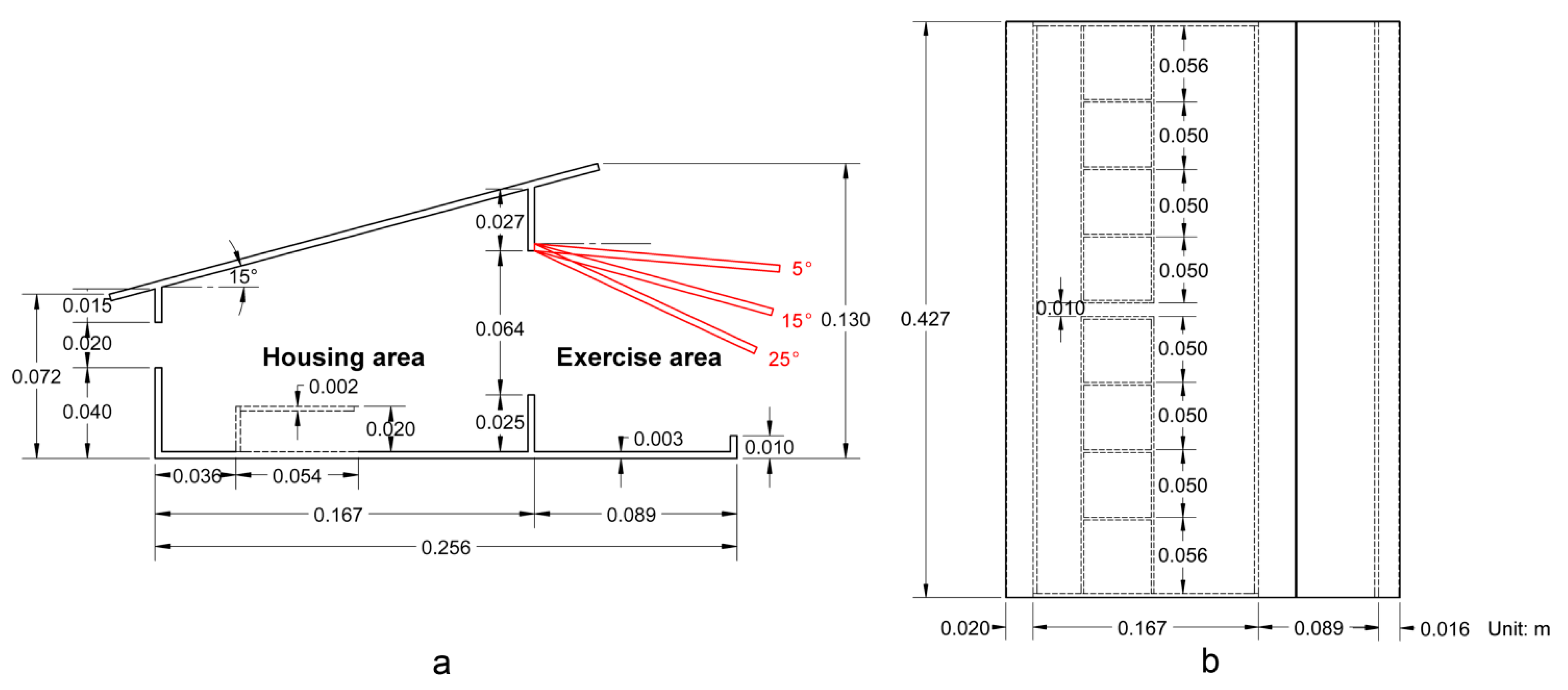
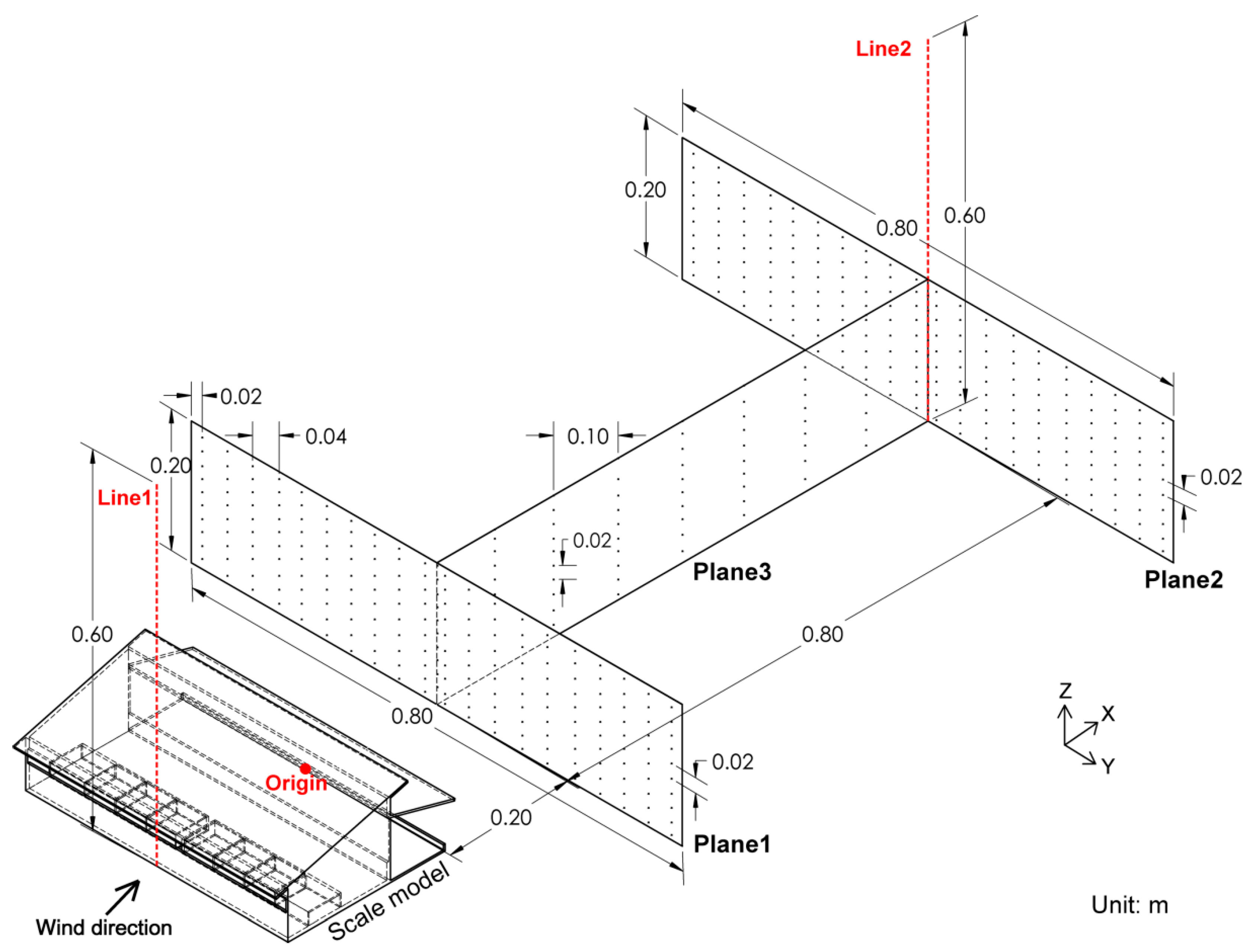
2.1. Scaled Pig Building Model

A scaled model of a naturally ventilated pig building with an outdoor exercise yard was used in this study. The prototype pig barn, situated in the state of Lower Saxony in northwest Germany, was designed for rearing around 80 fattening pigs. The scaled model was a 1:50 geometric reduction of the full-scale pig barn and was constructed at the Leibniz Institute for Agricultural Engineering and Bioeconomy (ATB), Germany.

The scaled model was made of transparent acrylic glass and consisted of an indoor housing area and an outdoor exercise area. The external dimension of the model was 0.427 m (length) × 0.256 m (width) × 0.130 m (height). The housing area had two sidewall openings with opening heights of 0.020 m and 0.064 m, respectively. Eight pigpens with open pen fronts were placed in the housing area. The height and width of all pigpens were 0.020 m and 0.054 m, respectively. The length of the two pigpens located next to gable walls was 0.056 m, and of other pigpens was 0.050 m. Pigpen walls had a thickness of 0.002 m, and all other walls of the building model had a thickness of 0.003 m. The roof of the building housing area had a fixed slope of 15°. The free access between indoor and outdoor areas through plastic strips or rotating doors in the prototype pig barn was constructed by a 0.025 m high acrylic sheet in the scaled model. The outdoor exercise area had a flexible roof with a length of 0.108 m and with a fixed top part, which totally covered the outdoor yard. There was a 0.010 m high sidewall but were no gable walls in the outdoor area. The prototype pig building was constructed to direct the excretion behaviour of pigs to the outdoor exercise yard [32], in which solid floors in the housing area and slatted floors with a deep pit in the outdoor area were adopted. Therefore, in this study we only considered the roof slope variations for the outdoor area, where the majority of emissions are expected to come from. Three cases with roof slopes of 5°, 15°, and 25° were studied in this paper. It has been found that the presence of animals has an insignificant impact on the airflow and pollutant dispersion within the barn [33], therefore, pigs and other internal structures that have smaller dimensions than the group of pigs, such as feeders, drinkers, metal bars, and slatted floors are expected to have minor influences on the airflow field downwind of the building. To simplify the model construction, pigs and these internal structures were not constructed. Detailed dimensions of the scaled pig building model and the three roof slope variations are illustrated in Figure 1.

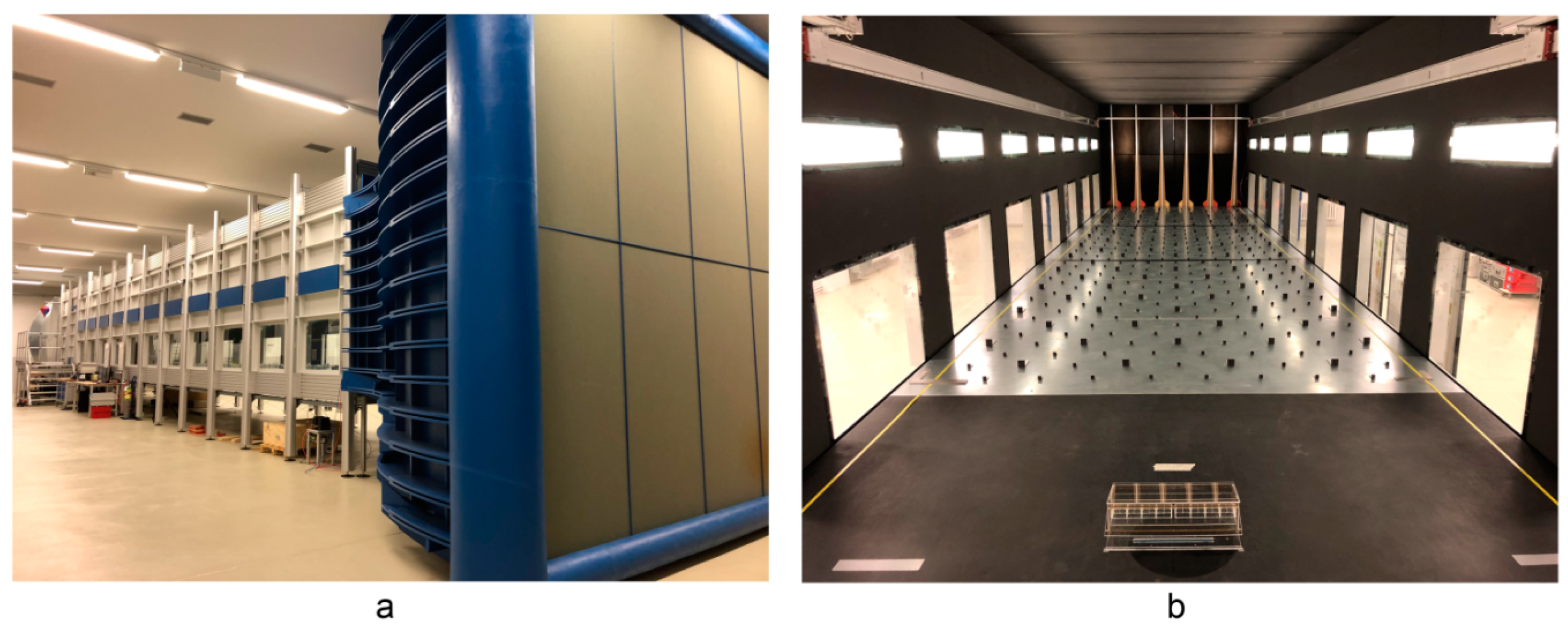
2.2. Boundary Layer Wind Tunnel and Measurement Devices

The experiments were carried out in a large boundary layer wind tunnel (BLWT) at ATB, Germany. The BLWT was specially designed to investigate ventilation and dispersion processes in agricultural buildings [34,35,36,37], and has also been used to generate datasets for CFD validation [24,38,39]. The wind tunnel is 28.5 m long, consisting of an air inlet fitted of honey combs, an air outlet equipped with an axial fan, and a 19.5 m-long test section. The cross-sectional area of the test section is 3 m (width) × 2.3 m (height). A combination of six spires and roughness elements was used to create a boundary layer flow. The spires were installed at the entrance of the test section. The roughness elements consisting of two sizes of right-angled steel brackets, with dimensions length × width × height of 0.010 m × 0.004 m × 0.004 m and 0.004 m × 0.002 m × 0.002 m for small and big brackets respectively, were arrayed in staggered rows downstream the spires. The total length of the roughness elements was 9.6 m with 0.2 m space between each row. The 1:50 scaled pig building model was placed at the symmetry line of the wind tunnel at 1.2 m downstream from the roughness elements. The model was oriented with sidewall openings perpendicular to the approaching flow and the outdoor yard at the downwind side. The blockage ratio of the scaled model to the cross-section of the wind tunnel was 0.8%, which is far less than the recommended maximum value of 5% for wind tunnel tests in VDI-guideline 3783/12 [40], and thus the tunnel effect can be neglected. Figure 2 shows photographs of the wind tunnel with the scaled model placed inside.

The free stream wind speed at the wind tunnel inlet (U_inlet) was measured using a Prandtl tube, connected to a pressure transducer MKS Baratron^® Type 120A (MKS Instruments, Andover, USA). The Prandtl tube was located at the centre of the entrance of the test section at a height of 1.3 m from the wind tunnel floor. Air velocity and turbulence around the scaled model were measured using a 2D fibre-optic Laser Doppler Anemometer (LDA) (Dantec Dynamics, Skovlunde, Denmark) combined with the BSA Flow Software package (Dantec Dynamics, Skovlunde, Denmark). The LDA probe head was 0.06 m in diameter and 0.45 m in length and provided a focal length of 0.25 m. The LDA probe was mounted on a three-dimensional computer-controlled traverse system that allowed automated and precise probe positioning with an uncertainty of <0.1 mm. A fog generator Tour Hazer II (Smoke Factory, Burgwedel, Germany) was placed at the wind tunnel inlet to produce seeding particles for LDA measurements. The temperature, relative humidity, and static pressure of the ambient air were measured using a FHAD 46x sensor with ALMEMO^® D6 plug (AHLBORN Mess- und Regelungstechnik GmbH, Ilmenau, Germany). The data were sampled approximately every hour. The mean values of temperature, relative humidity, and static pressure for each day were used to calculate the air density, and therefore to calculate the U_inlet by using together with the data from the Prandtl tube.

2.3. Measurement of Boundary Layer Profile

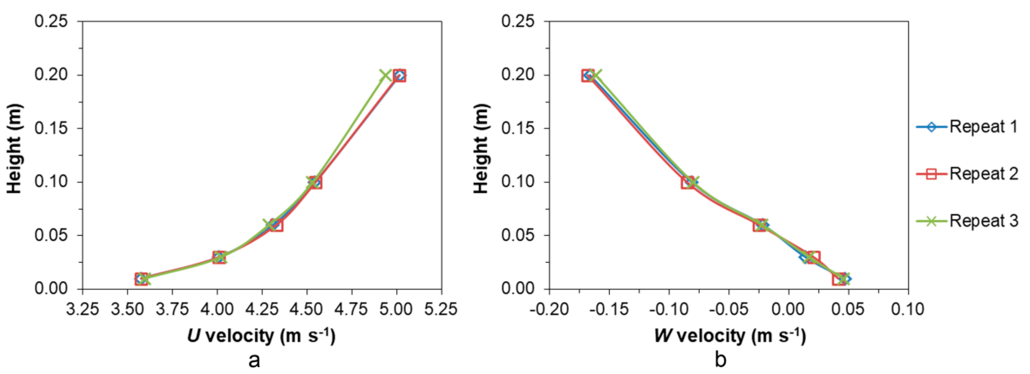
2.3.1. Reynolds Number Independence Study

In order to obtain a fully developed turbulent flow in the wind tunnel, a Reynolds number independence study for the approaching flow was carried out. The wind profile was measured at 20 positions along a vertical line ranging from 0.003 m to 0.6 m above the wind tunnel floor at the upstream edge of the scaled model (i.e., at Line 1 in Figure 3). The wind profile measurements were performed without the presence of the scaled model at free stream wind speeds (U_inlet) of 4, 6, 8, 10, and 12 m·s⁻¹, respectively. The streamwise (U) and vertical (W) velocity components were measured using the 2D LDA. The measurements at each measurement position were taken continuously until the sampling number reached 40,000 readings or the maximum sampling time reached 820 s before moving the LDA probe to another position. The average sampling rate during experiments was around 300 s⁻¹. A 10s pause between each measurement position was set in order to minimise the disturbance of the movement of the LDA probe to the flow field. The above LDA setup was chosen according to a preliminary experiment for the reproducibility of statistic results, in which air velocities at heights of 0.01 m, 0.03 m, 0.06 m, 0.1 m, and 0.2 m along Line 1 were measured and repeated three times at U_inlet of 8 m·s⁻¹. The results showed that with this setup the measurement uncertainty for the time-averaged U and W velocities was 0.3%, and 5.5%, respectively (Figure 4). The above mentioned LDA setup was used for all air velocity measurements in this study.

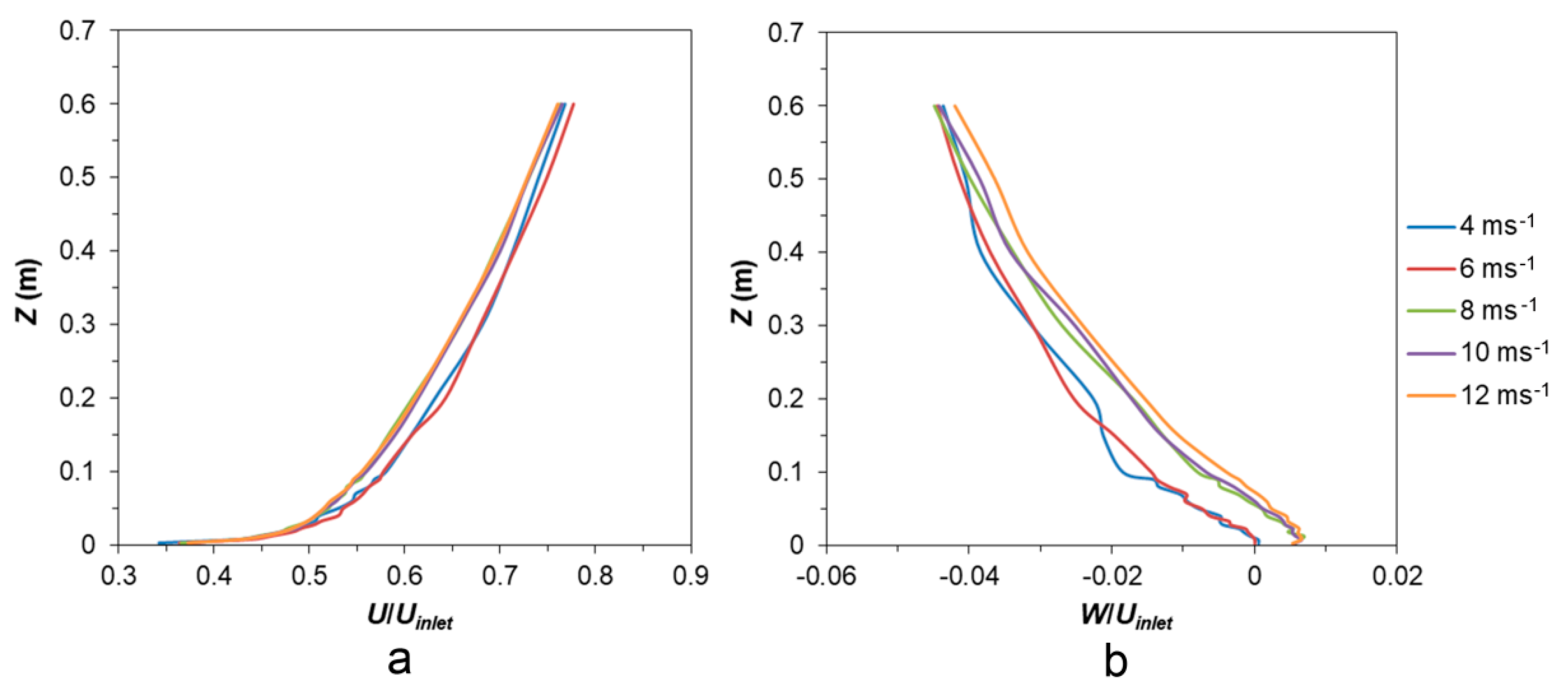
2.3.2. Stability Study

To establish a stable boundary layer airflow that represents a farmland terrain, the characteristics of wind profiles within the region of interest were assessed. The arrangement of the roughness elements was adjusted accordingly until reaching a desirable boundary layer flow following the VDI-guideline 3783/12 [40]. Air velocities at two vertical lines, one at the upstream edge of the scaled model (i.e., Line 1 in Figure 3) and the other at the downstream end of the region of interest (i.e., Line 2 in Figure 3), from 0.003 m to 0.6 m height along the symmetry line of the model were measured. Measurements were carried out using the 2D LDA without the presence of the scaled model. Free stream wind speed in the wind tunnel was 8 m·s⁻¹. Parameters that define the roughness class of the boundary layer, e.g., the wind profile power exponent, roughness length, and turbulence intensity were examined.

2.4. Measurement of Airflows Downwind the Building

In order to investigate airflow characteristics and to predict air pollutant dispersion properties downwind the building, air velocities at three vertical planes (Planes 1–3, Figure 3) downwind the 1:50 scaled pig building model were measured with the LDA. Streamwise and vertical velocity components were measured simultaneously. Mean and instantaneous air velocities were recorded to obtain average and turbulent airflow information. Plane 1 and Plane 2 were parallel to the building sidewalls at separation distances of 0.2 m (corresponded to 10 m in full-scale) and 1.0 m (corresponding to 50 m in full-scale) downwind the building model, respectively. Both Plane 1 and Plane 2 had a dimension of Y × Z = 0.8 m (width) × 0.2 m (height), each consisting of 200 velocity measurement points with 10 points in each vertical line and 20 points in each horizontal line. Plane 3 was positioned along the symmetry plane of the scaled model with a dimension of X × Z = 0.8 m (length) × 0.2 m (height), including 90 measurement positions distributed at 9 vertical lines. In this study, X, Y and Z denoted the axes of the coordinate system, which were aligned with the streamwise, spanwise and vertical wind directions, respectively. The origin of the coordinate system was located at the centre of the downstream edge of the scaled model at the wind tunnel floor. The airflow measurement positions and the definition of the coordinate system are depicted in Figure 3. According to the wind profile measurement results (described in Section 3.1), a stable and fully developed turbulent flow that represents a farmland terrain boundary layer could be obtained when the free stream wind tunnel speed (U_inlet) was at least 8 m·s⁻¹. Therefore, all airflow measurements downwind the scaled model were performed at U_inlet of 8 m·s⁻¹.

2.5. Data Analysis

The mean and the standard deviation of the air velocity in streamwise and vertical directions at each measurement position were provided by BSA Flow Software (Dantec Dynamics, Skovlunde, Denmark). Air velocity and air turbulence characteristics were processed from 40,000 samples at each position to ensure statistically reliable results.

The velocity magnitude calculated from two-dimensional velocity components was defined as:

$$V_{2D}=\sqrt{U^2{+W}^2}$$

(1)

where V_2D is the velocity magnitude, m·s⁻¹; U and W are mean air velocities in streamwise and vertical directions, respectively, m·s⁻¹.

Turbulence intensity and turbulent kinetic energy of the airflow were calculated by Equations (2) and (3), respectively.

$$TI=\sqrt{0.5\left({\sigma }_U^2{+\sigma }_W^2\right)}/V_{2D}\times 100\%$$

(2)

$$TKE=0.5\left({\sigma }_U^2{+\sigma }_W^2\right)$$

(3)

where TI is the turbulence intensity, %; TKE is the turbulent kinetic energy, m²·s⁻²; V_2D is the velocity magnitude, m·s⁻¹; σ_U and σ_W are standard deviations of the instantaneous air velocity in streamwise and vertical directions, respectively, m·s⁻¹.

It is noted that in this study V_2D, TI, and TKE were calculated based on a two-component velocity analysis.

3. Results and Discussion

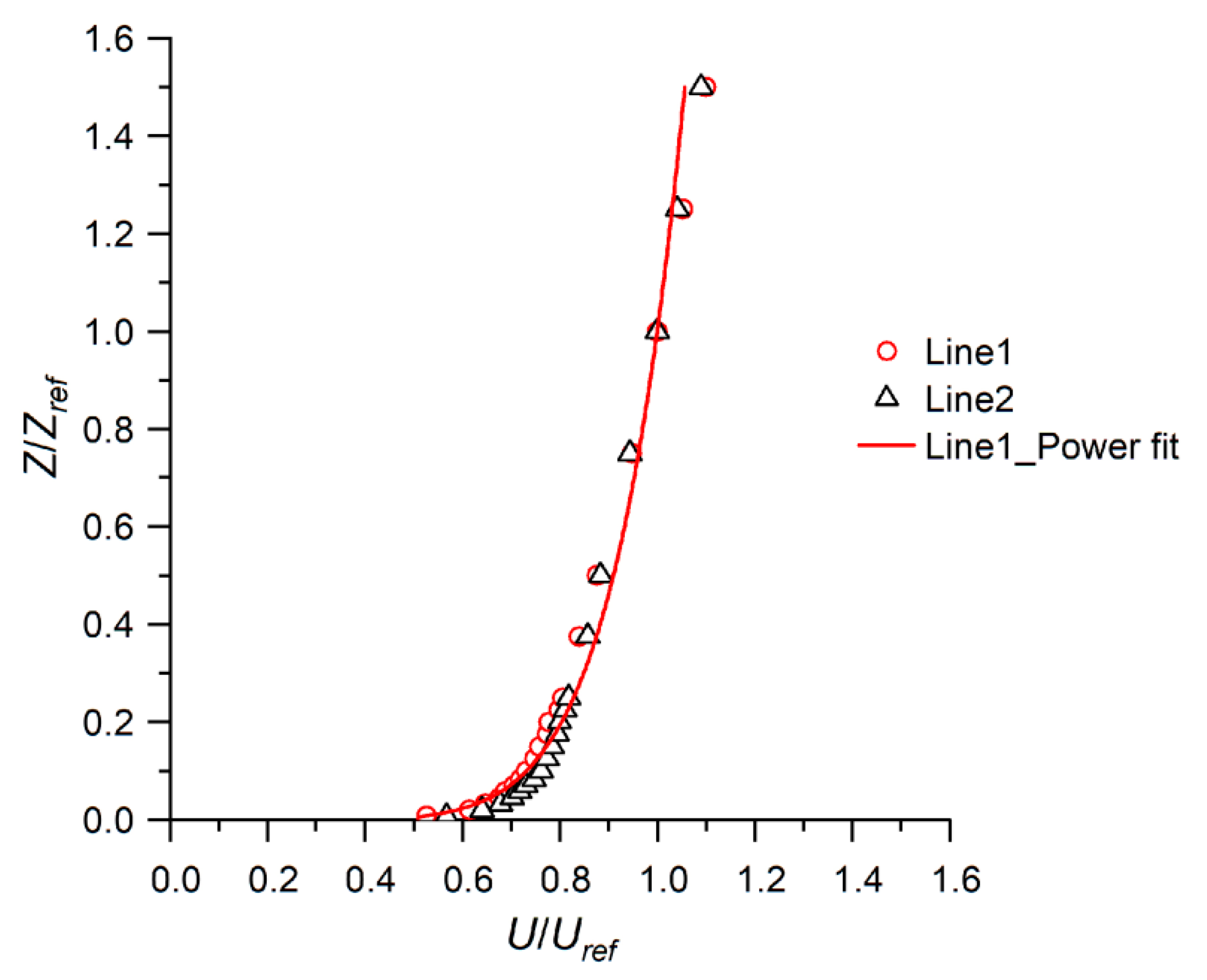
3.1. Boundary Layer Profile

3.1.1. Reynolds Number Independence Study

Dimensionless streamwise (U/U_inlet) and vertical (W/U_inlet) velocity profiles in the vertical direction (Z) at Line 1 in Figure 3 are compared in Figure 5 for different free stream wind speeds at the wind tunnel inlet (U_inlet), in order to identify the critical U_inlet above which the flow can be considered Reynolds number independent [41]. The results showed that under U_inlet of 4 m·s⁻¹ and 6 m·s⁻¹ conditions, the values of both U/U_inlet and W/U_inlet were different to the other cases. When U_inlet increased from 6 m·s⁻¹ to 8 m·s⁻¹, the average relative change of dimensionless air velocities was 0.391 and 0.006 for U/U_inlet and W/U_inlet, respectively. In contrast, when U_inlet increased from 8 m·s⁻¹ to 10 m·s⁻¹, the average relative change was only 0.003 and 0.001 for U/U_inlet and W/U_inlet, respectively. It indicated that when U_inlet exceeded 8 m·s⁻¹, the dimensionless wind profile did not change considerably with further increase of the wind tunnel wind speed. Therefore, the Reynolds number independence was reached and a fully-developed turbulent flow was obtained at U_inlet of 8 m·s⁻¹.

3.1.2. Stability Study and Wind Profile Properties

To ensure a stable airflow within the region of interest, wind profiles at the upwind edge of the model (Line1) and the end of downwind airflow measurement region (Line 2) were measured without the scaled model. The vertical profiles of the streamwise air velocity component for Line 1 and Line 2 are compared in Figure 6. The results showed that the two profiles agreed well with each other with an average relative difference of 3.5%, indicating that a stable airflow was achieved within the region of interest.

Figure 6 showed that the mean streamwise air velocity profile of the incident flow (i.e., at the upwind edge of the model) in the vertical direction followed a power law with the exponent of 0.14 and the coefficient of determination R² of 0.98:

$${U=U}_{ref}{\left(Z/Z_{ref}\right)}^{0.14}$$

(4)

where U and U_ref are the mean streamwise air velocity at height Z and a reference height Z_ref, respectively, m·s⁻¹. To achieve the best fit of the model for the air velocity profile, U_ref = 5.55 m·s⁻¹ and Z_ref = 0.4 m were chosen in this study.

The streamwise air velocity at the building height (U_B), calculated by Equation (4), was 4.77 m·s⁻¹. This resulted in a building Reynolds number (Re_B) of 53,759, which was calculated by Equations (5) and (6).

$${Re}_B{=U}_B·D/\nu$$

(5)

$${D=2W}_B·Z_B/\left(W_B{+Z}_B\right)$$

(6)

where ν is the kinematic viscosity of the air, m²·s⁻¹; D is the characteristic length of the scaled pig building model, calculated as the hydraulic diameter of the cross-section of the model, m; W_B and Z_B are the width and the height of the scaled model, respectively, m. The average ambient temperature and relative humidity during the whole experimental period were 22.4 °C and 34.2%, respectively. Therefore, ν took the value of 1.53 × 10⁻⁵ m²·s⁻¹ at temperature of 22.4 °C.

By fitting the air velocity profile of the incident flow to a logarithmic law, it gave the friction velocity (u*) of 0.22 m·s⁻¹ and the full-scale roughness length (z₀) of 6.4 × 10⁻³ m, in which the von Karman constant took the value of 0.4. This gave the roughness Reynolds number (Re_z0) of 92, which was calculated according to Equation (7).

$${Re}_{z0}{=u}^{*}·z_0/\nu$$

(7)

It is stated in the VDI-guideline [40] that a moderately rough (corresponds to grassland or farmland) turbulent boundary layer should meet the following requirements: the profile power law exponent falls within the region of 0.12–0.18, and the roughness length within 0.005–0.1 m. In this study, both the power exponent of 0.14 and z₀ of 6.4 × 10⁻³ m satisfied the aforementioned criteria, hence the generated boundary layer can be considered to represent the airflow over farmland terrain.

Additionally, both the building Reynolds number (Re_B) of 53,759 and the roughness Reynolds number (Re_z0) of 92 were considerably higher than the reported critical Re_B of 4000 [42] and critical Re_z0 of 2.5 [43], respectively for a Reynolds number independent flow. It further indicated that the airflow generated in our wind tunnel at U_inlet of 8 m·s⁻¹ was fully developed turbulent.

Therefore, all subsequent measurements were performed at U_inlet of 8 m·s⁻¹.

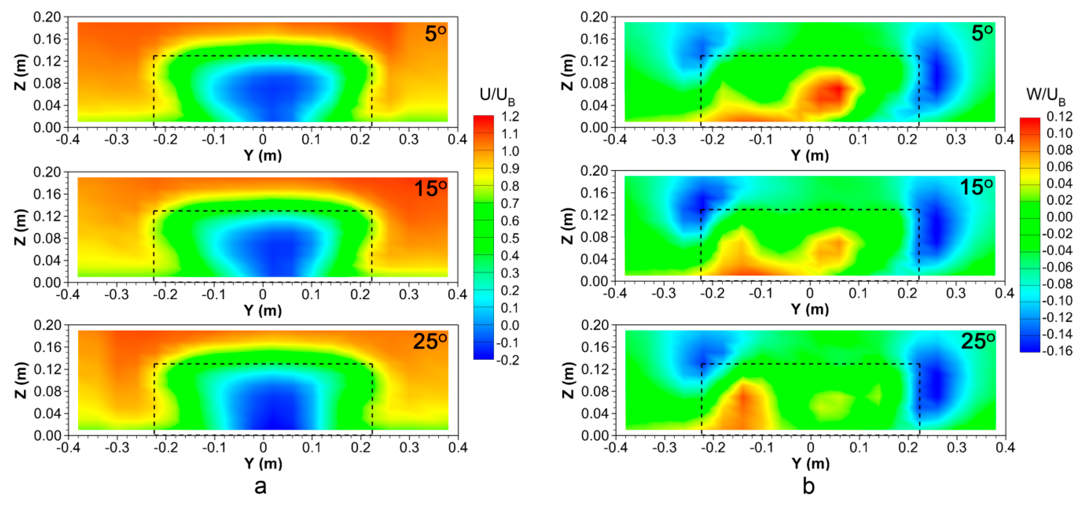
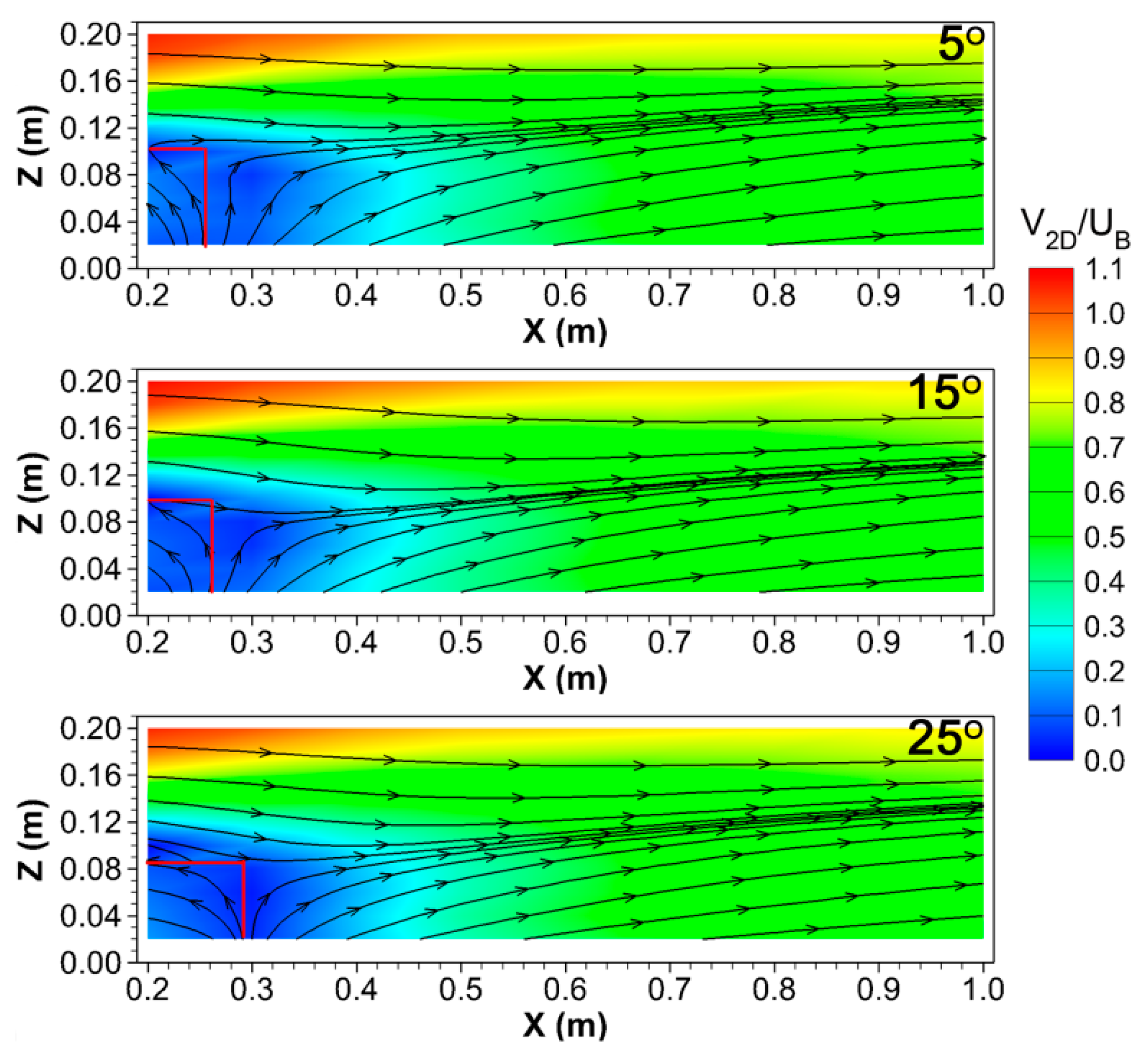
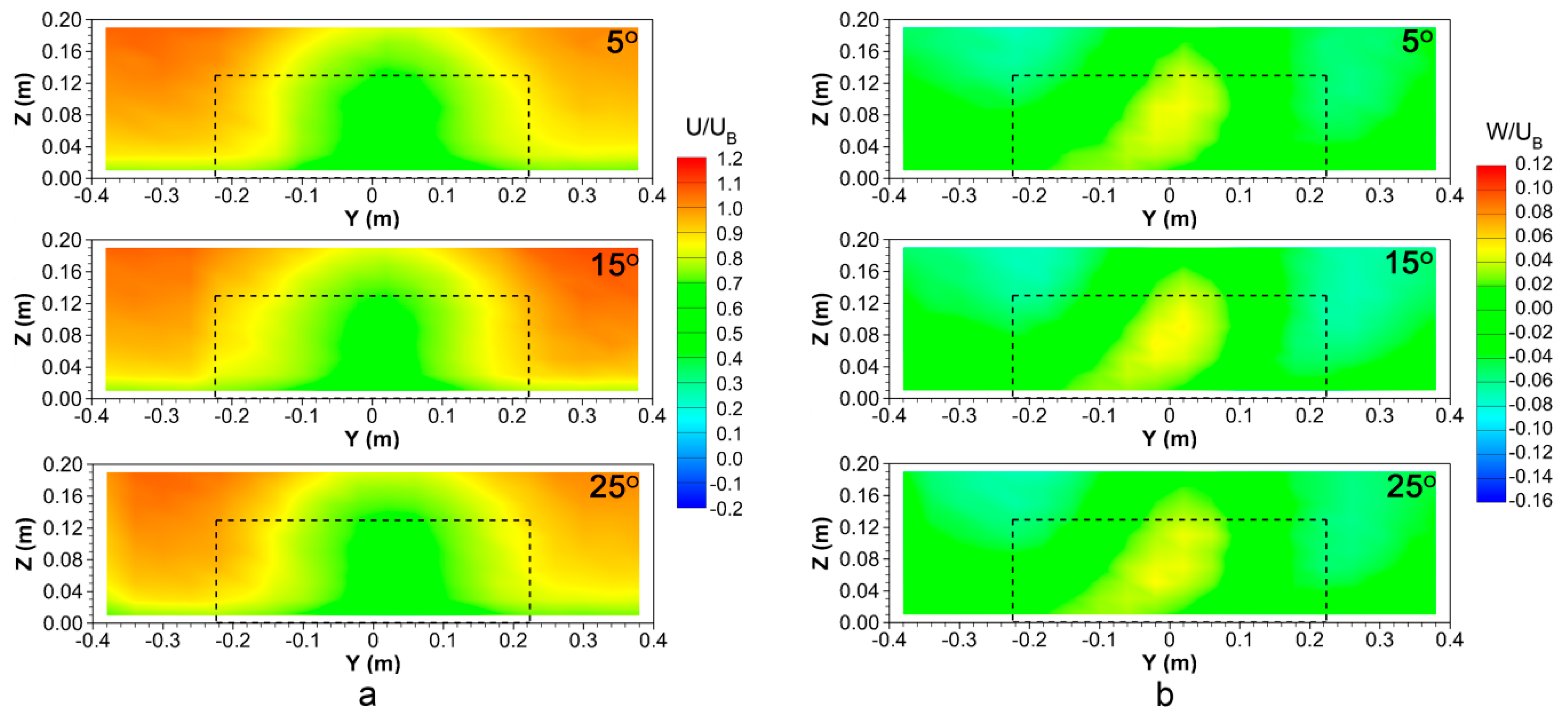
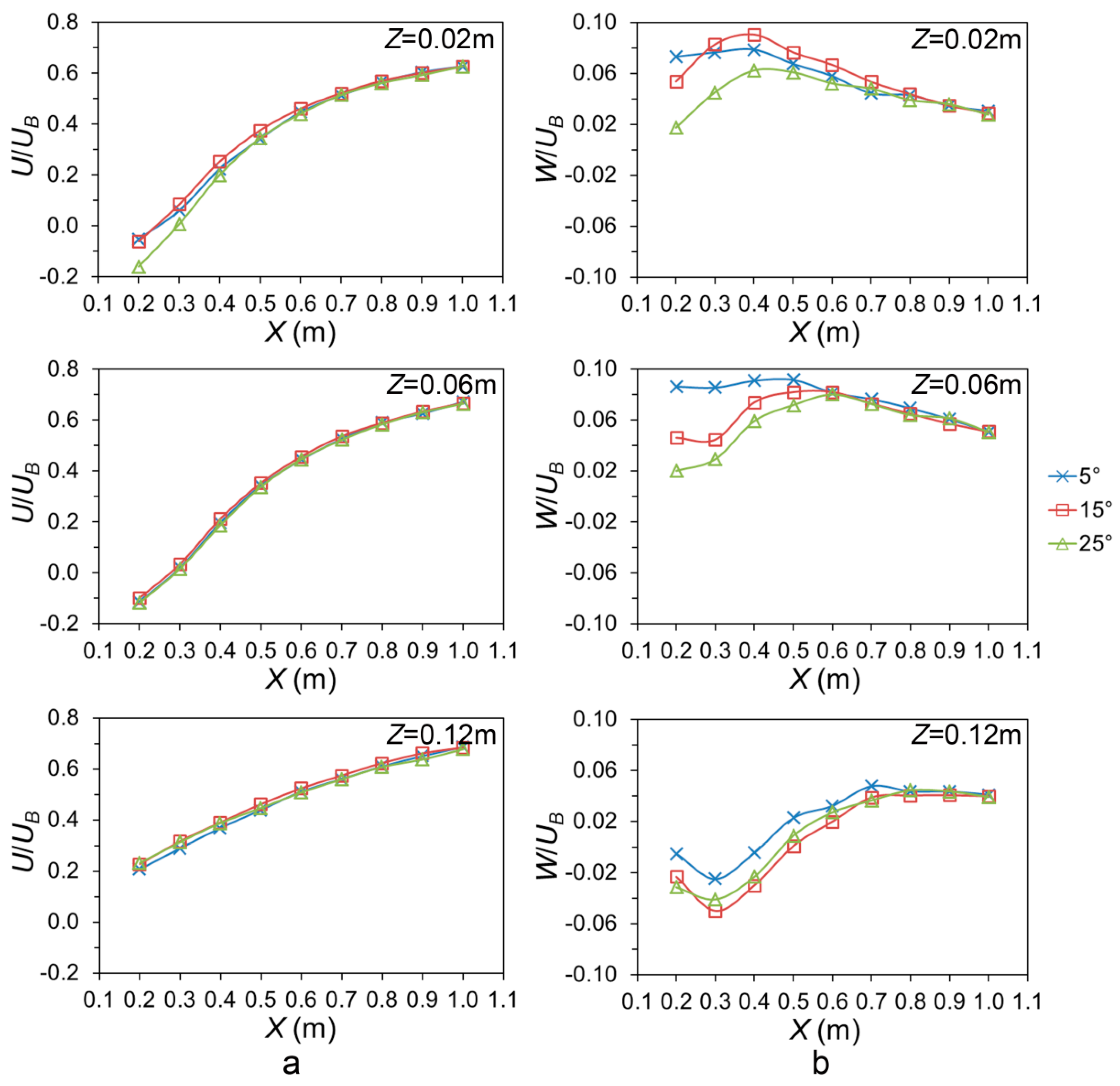
3.2. Mean Air Velocities Downwind the Building

Figure 7a shows contours of mean streamwise air velocity normalised by the air velocity at the building height (U_B) at Plane 1 for three roof slopes of the exercise yard of the scaled pig building model. Considerably lower air velocities were observed right behind the building with negative values in the centre (represented in dark blue in Figure 7a). The negative U velocities indicated reverse flows through Plane 1, which occurred slightly below the building height. The region of the reverse flow was affected by the roof slope in the spanwise wind direction (Y). It became narrower in the upper part but wider in the lower part for a steeper roof. Beyond the reverse flow region, the air flowed towards downstream with a reduced air velocity. Figure 7b compares the dimensionless mean vertical air velocity contours at Plane 1 for roof slopes of 5°, 15°, and 25°. It was found that at both sides of the building, W velocities were negative, which indicated a downward flow direction. In contrast, within the region right behind the building upward airflows were observed. This indicated a complex three-dimensional air movement downwind the building caused by the air passing through and around the building. It is noted that the velocity contours were not strictly symmetric even though the scaled model was geometrically symmetric and the wind direction was perpendicular to the model sidewalls. The most possible reason for the asymmetrical airflow contours was the disturbance of the LDA probe to the flow field when it was positioned close to the building. The cross-sectional area of the LDA probe was 0.003 m², accounting for 5% blockage to the airflow at the position right behind the building. This was not intended but was unavoidable, restricted by the focal length of the LDA. The potential influence of the air velocity sensor to the airflow was also reported by Sauer et al. [25], who observed an asymmetrical air velocity pattern at a vertical plane downstream from four aligned swine building models measured using a 3D hot-film anemometer. The results raised a potential interesting topic that is to quantify the disturbance of the LDA probe to the flow field, which could be done with CFD simulations.

Figure 8 depicts contours of dimensionless streamwise and vertical air velocities at Plane 2 for the three roof slopes. Lower air velocities at the position behind the building than around the building were still observed. This indicated that the presence of the building affected the airflow field at a distance of 1.0 m (i.e., 7.7Z_B, where Z_B is the building height, corresponding to 50 m in full scale) downwind the building. In contrast to Plane 1, no reverse flows occurred at Plane 2 for all three cases. It was found that U velocities right behind the building at Plane 2 were obviously higher than those at Plane 1. However, Plane 1 presented higher air velocities at the height above 0.16 m than Plane 2 (Figure 7a and Figure 8a), which was caused by the wind shear effect that accelerated the air when the air flowed over the top of the building. Compared with Plane 1, Plane 2 presented a more homogeneous vertical air velocity pattern with slightly upward airflows occurring near the centre (Figure 8b). Only small differences among different roof slope cases for both U and W velocities at Plane 2 were observed. It demonstrated that the slope of the leeward roof did not considerably affect the airflow at Plane 2.

Airflow streamlines and contours of the air velocity magnitude (V_2D) normalised by U_B at Plane 3 for the three roof slopes are compared in Figure 9. The axes X and Z indicate the downwind distance to the building and the height from the wind tunnel floor, respectively. There was an elliptic-shaped low air velocity region with V_2D/U_B of smaller than 0.4 behind the building with a height of 0.13 m (i.e., 1Z_B) and a downstream distance of 0.5 m (i.e., 3.8Z_B and corresponding to 25 m in full-scale) for all three roof slopes. This region is expected to have a high concentration of air pollutants. This is because airborne pollutants are mainly transported by mean airflow, which results in the concentration of pollutants being inversely related to the air velocity downwind the building if no recirculation regions are presented [44]. If applying additional air pollutant treatment technologies, for example using pollutant traps or sprinklers to collect or wash high-concentrated air pollutants in this low air velocity region might effectively mitigate air contaminants and release their burden to the surrounding environment and residents. Additionally, within this low air velocity region, a wake zone with reversed airflow was observed at Plane 3, implying an anti-clockwise air recirculation in which air pollutants would accumulate. The size and shape of the wake was affected by the roof slope. For the roof slope of 5°, 15°, and 25°, the wake height (in Z direction) was 0.103 m, 0.099 m, and 0.084 m, respectively. Accordingly, the wake length (in X direction) was 0.254 m, 0.261 m, and 0.290 m, respectively. It showed that the larger the roof slope was, the lower and longer the wake became, and vice versa. As a result, the accumulated air pollutants would disperse farther for a steeper roof slope. The wake length observed by Tominaga et al. [23] was 2.5Z_B and 2.8Z_B for a gable-roof building (without openings) with the roof slope of 16.7° and 26.6°, respectively, which is slightly greater than 2.0Z_B and 2.2Z_B for the roof slope of 15° and 25° respectively obtained in our study. This is because the sealed building structure could result in a much lower pressure field behind the building and thus a larger air recirculation region. In contrast to the results in this paper where the wakes were found from the floor level until above the roof, in a wind tunnel study of Ikeguchi and Okushima [18] using naturally ventilated dairy building models without outdoor exercise yards, the wakes were only observed above the leeward roof. One possible reason could be the large sidewall openings used in their study, which resulted in a cross ventilation through the building. In contrast, in our study, a small slot inlet opening with a high sidewall led to an up-jet airflow pattern inside the housing area. Additionally, the exercise yard with an upwind sidewall further complicated the airflow and resulted in the reversed flow behind the building. Therefore, our results are expected to be applicable to naturally ventilated livestock buildings with small inlet openings and downwind outdoor yards in a perpendicular wind direction.

Figure 10 shows the variations of the dimensionless air velocities with distance to the building at heights (Z) of 0.02 m, 0.06 m, and 0.12 m, which corresponded to 1 m, 3 m, and 6 m in full-scale. At Z of 0.02 m, the roof slope of 25° resulted in lower U/U_B and W/U_B velocities than roof slopes of 5° and 15° until a distance of around 0.7 m from the building. At Z of 0.06 m and 0.12 m, there were not many differences for U/U_B velocities among the three roof slopes. However, for W/U_B velocities, the 5° roof slope presented the highest values among three cases until a distance of 0.6 m at Z of 0.06 m and a distance of 0.8 m at Z of 0.12 m, respectively, indicating a more upwards airflow direction. At a distance beyond 0.8 m (i.e., 6.2Z_B) from the building, the roof slope had almost no effect on the air velocities. This is in line with the previous observations at Plane 2 shown in Figure 8 where no considerable differences could be detected among three roof slope cases.

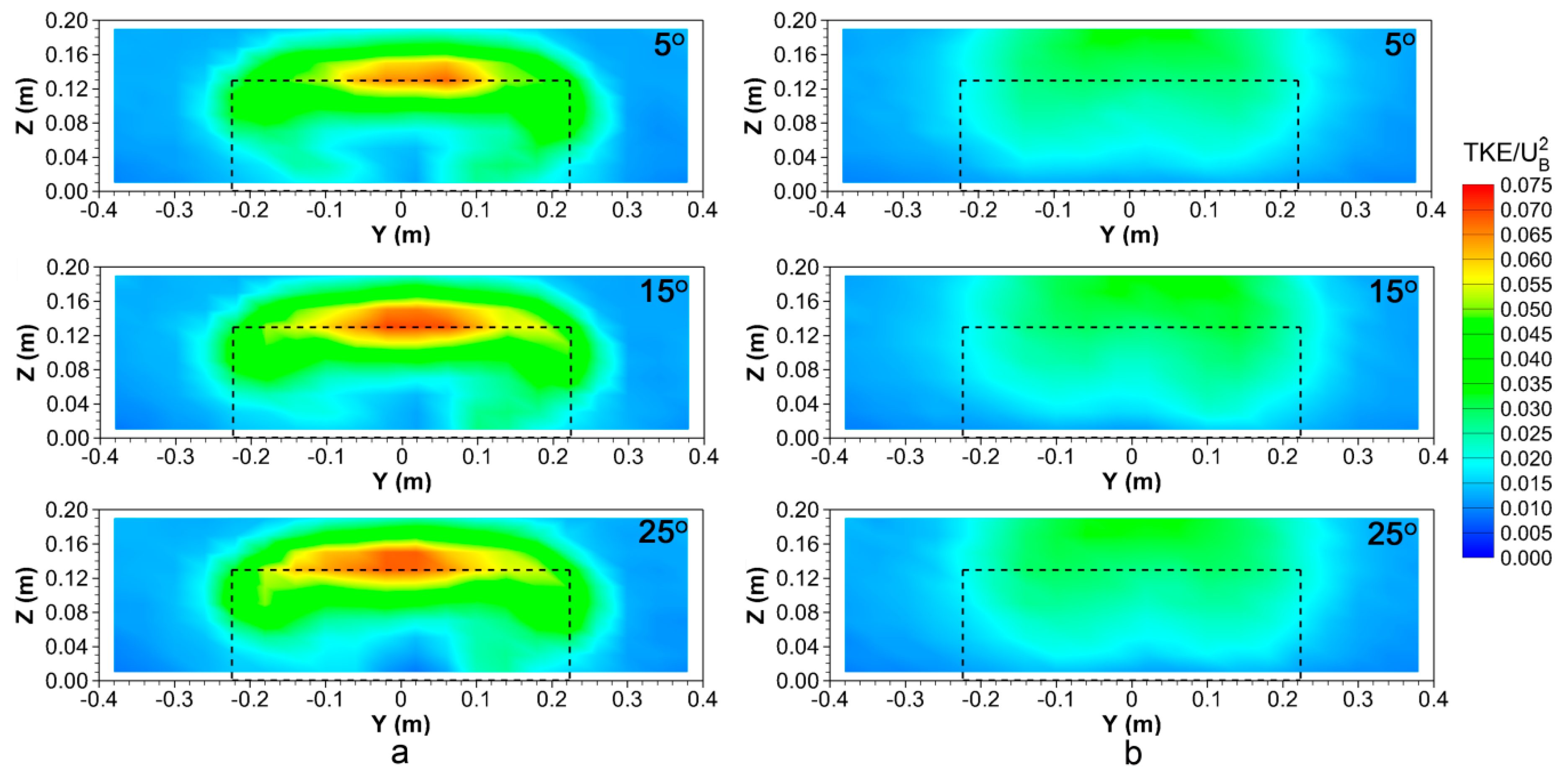
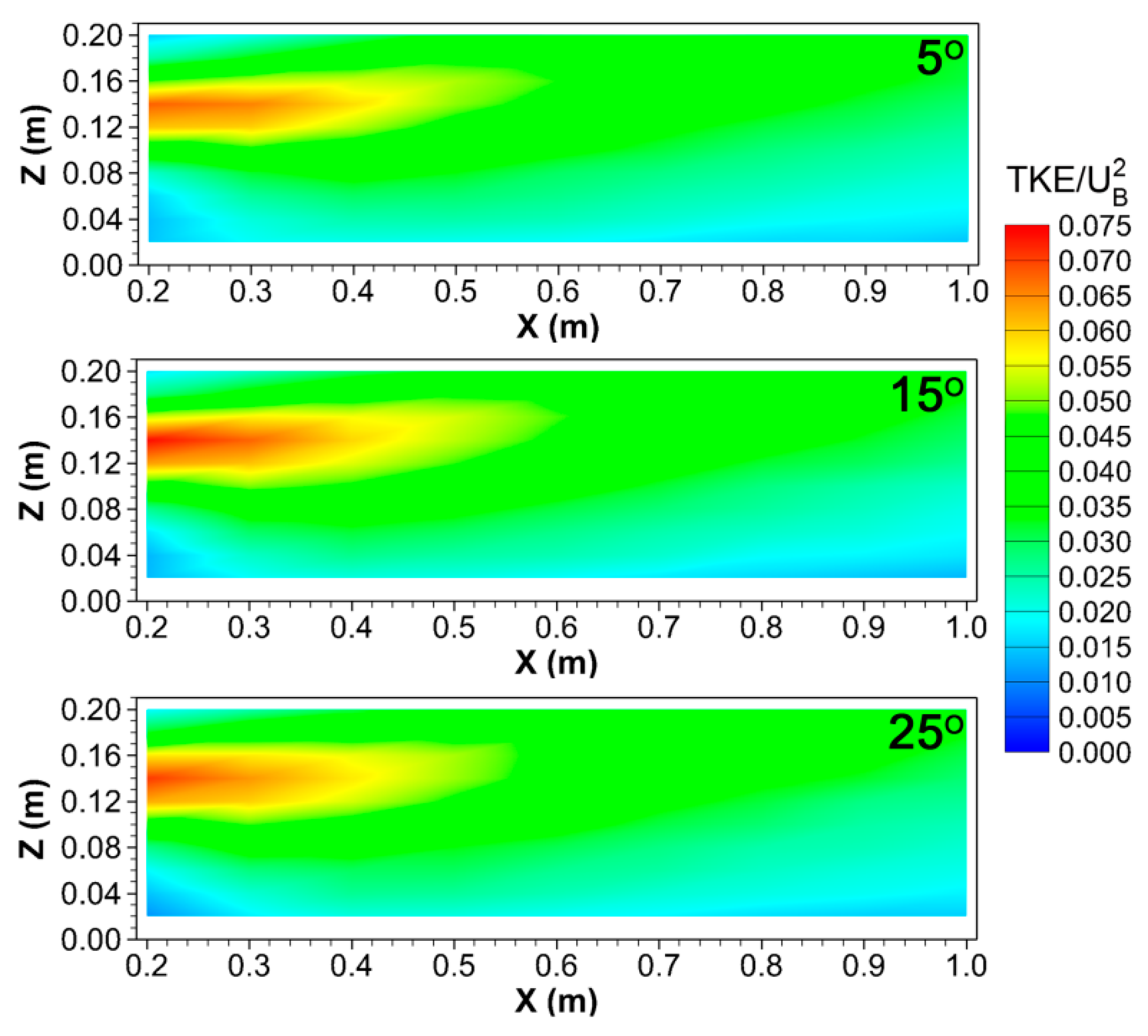
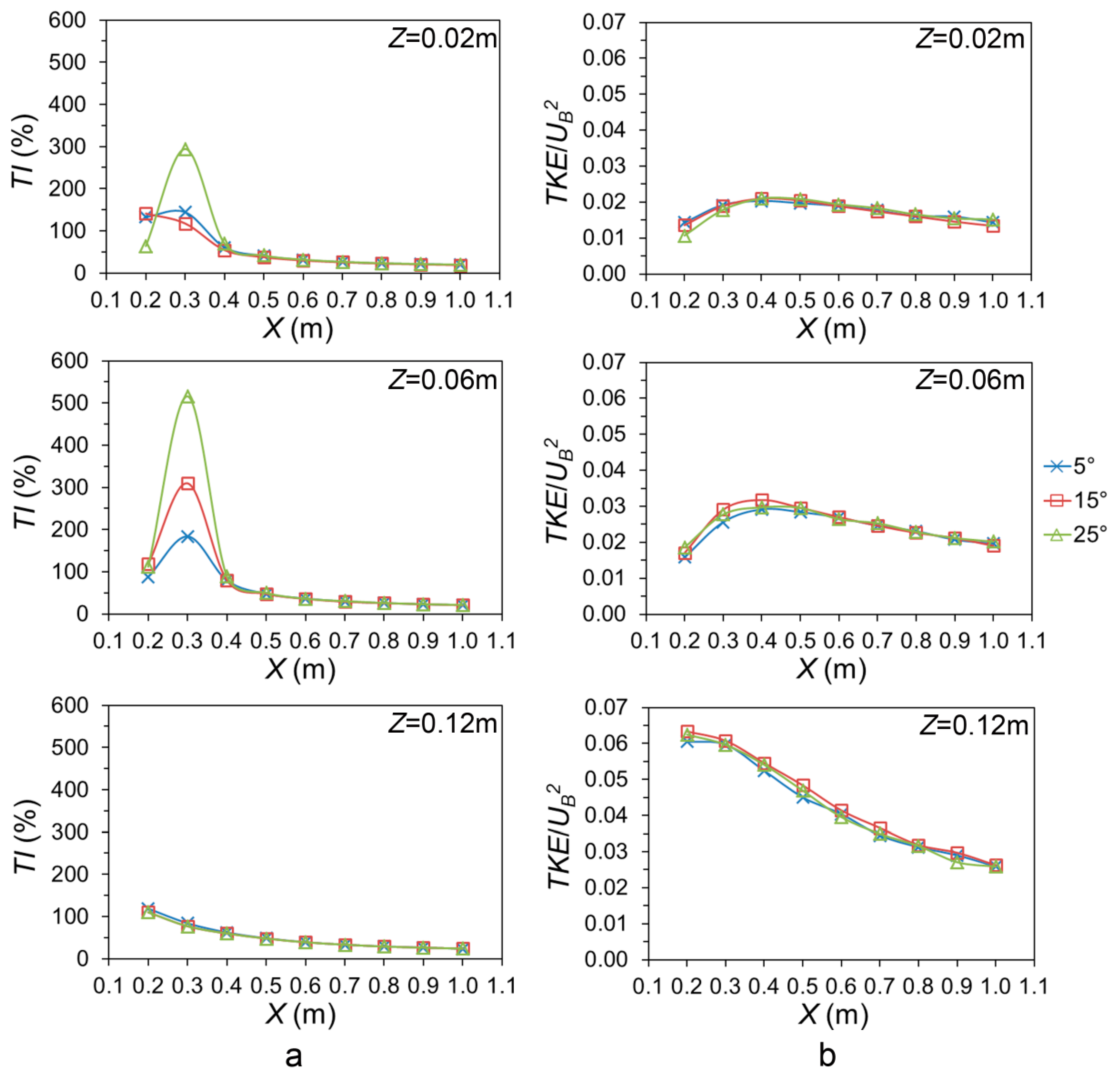
3.3. Air Turbulence Downwind the Building

Spatial distributions of the turbulent kinetic energy (TKE) normalised by the square of the streamwise air velocity at the building height (U_B) at Plane 1 and Plane 2 for roof slopes of 5°, 15°, and 25° are compared in Figure 11. It was found that TKE had different patterns from air velocities, where the region of low air velocities generally presented higher TKE values. At Plane 1, the highest TKE occurred at the centre of the building around the building height. This might be caused by the air collision of the reverse flow occurred in the wake and the bulk air flowed over the building, which increased the air turbulence in that region. At Plane 1, the high TKE region was the smallest when the roof slope was 5°. At Plane 2, higher TKE was observed behind and above the building than in other areas. It indicated that the influence of the building on the downwind air turbulence reached Plane 2. Only minor TKE pattern differences among different roof slopes were observed at Plane 2, which implied that the roof slope had almost no effects on TKE at Plane 2.

Figure 12 illustrates the normalised TKE distributions at Plane 3 for three roof slopes. The highest TKE was observed in the region in the vicinity of the building height. It decayed gradually as the distance to the building increased. The high TKE region that is represented in red and yellow in Figure 12 extended up to approximately 0.5 m (i.e., 3.8Z_B) downwind from the building. It was located right above the region in which the air velocity was low (as depicted in Figure 9). This could be attributed to the flow reattachment on the leeward roof that led to the production of TKE. Ntinas et al. [45] also found a high turbulence production in the air recirculation region behind the scaled model. It is known that the transport of airborne pollutants is affected by both the mean air velocity and the air turbulence [46]. Therefore, in that low air velocity region, the aerial pollutants would be likely transported via the energetic turbulent eddies/turbulence diffusion.

The influences of the roof slope on the air turbulence, denoted by the turbulence intensity (TI) and dimensionless turbulent kinetic energy (TKE/$U_B^2$), with respect to the downwind distance from the building (X) at heights (Z) of 0.02 m, 0.06 m, and 0.12 m are described in Figure 13. A considerably higher TI was found at X of 0.2 m–0.4 m for Z of 0.02 m and 0.06 m, where the air vortex was formed in the wake as depicted in Figure 9. The highest TI was observed in the most downward roof structure (i.e., roof slope of 25°), which was attributed to an enhanced disturbance of the roof to the airflow. At Z of 0.12 m, the TI had lower values compared with Z of 0.02 m and 0.06 m, and decreased slowly with distance from the building. The influence of the roof slope on the TI was negligible when the distance from the building exceeded 0.5 m (i.e., 3.8Z_B) (Figure 13a). The highest TKE/$U_B^2$ occurred at Z of 0.12 m and decayed gradually away from the building. Even though the roof slope had a big impact on the TI, no notable differences were observed among different roof slope cases for TKE/$U_B^2$, indicating that the variations in the leeward roof slope might have little influence on the turbulent kinetic energy of the airflow downwind the building. The same TKE/$U_B^2$ values for different cases implied that the velocity fluctuations, as explained by Equation (3), were not affected by the roof slope. However, the velocity magnitude (V_2D), which was calculated from the U and W velocities (Equation (1)) were affected by the roof slope, as seen in Figure 10. According to Equation (2), TI was calculated as the ratio of the square root of TKE to V_2D. Therefore, different TI values were observed among different roof slope cases although the same TKE/$U_B^2$ occurred.

4. Conclusions

Mean air velocity and air turbulence downwind a 1:50 scaled model of a naturally ventilated pig building with a totally roofed outdoor exercise yard with different roof slopes were measured in a large boundary layer wind tunnel to investigate downwind airflow characteristics and the related air pollutant transport and dispersion properties. Before the downwind airflow measurements, wind profile properties were examined to ensure a fully-developed turbulent flow in the wind tunnel. Based on the results obtained, the following conclusions could be drawn:

• Reduced air velocities were observed right behind the building. At the vertical plane parallel to the building sidewalls with a distance 0.2 m (i.e., 1.5Z_B, where Z_B is the building height) downwind the building, reverse flows occurred in the centre of the plane and were affected by the roof slope.
• An elliptic-shaped low air velocity region along the distance to the building was found. It had a similar height as the building and reached 0.5 m (i.e., 3.8Z_B and corresponded to 25 m in full-scale) downwind from the building. Within this region, the mean air velocities were low and thus might result in a higher gaseous pollutant concentration. This suggested that applying additional treatment technologies to trap the high-concentrated gaseous pollutants (e.g., odours or ammonia) in this region might contribute to the mitigation of pollutant emissions to the atmosphere and alleviation of the burden to the surrounding environment. Apart from the mean air velocity, the transport of the air pollutants in this region was likely attributed to the turbulent eddies.
• A wake zone with recirculated air was observed for all three roof slope cases. The larger the roof slope was, the lower and longer the wake zone became. It indicated that a steeper roof could result in the accumulated air pollutants dispersing to a farther distance.
• The effect of the roof slope to the mean air velocity and the air turbulence could reach up to distances of 0.8 m (i.e., 6.2Z_B) and 0.5 m (i.e., 3.8Z_B) downwind from the building, respectively.

To the best of our knowledge, the present study was the first to provide detailed information of the downwind airflow for a naturally ventilated pig building with totally roofed outdoor access. The airborne pollution transport and dispersion properties were predicted from the airflow characteristics. To support the findings, further research on the downwind gas concentration fields using a tracer gas will be conducted. The mean air velocity and air turbulence data provided in this paper can be used for validation of CFD models which permits more comprehensive studies on the effect of multiple factors on airflow patterns both indoors and around the building.

References

1. Stavrakakis, G.M.; Koukou, M.K.; Vrachopoulos, M.G.; Markatos, N.C. Natural cross-ventilation in buildings: Building-scale experiments, numerical simulation and thermal comfort evaluation. Energy Build. 2008, 40, 1666–1681. [Google Scholar] [CrossRef]
2. De Paepe, M.D.; Pieters, J.G.; Cornelis, W.M.; Gabriels, D.; Merci, B.; Demeyer, P. Airflow measurements in and around scale model cattle barns in a wind tunnel: Effect of ventilation opening height. Biosyst. Eng. 2012, 113, 22–32. [Google Scholar] [CrossRef]
3. Honeyman, M.S. Extensive bedded indoor and outdoor pig production systems in USA: Current trends and effects on animal care and product quality. Livest. Prod. Sci. 2005, 94, 15–24. [Google Scholar] [CrossRef]
4. Park, H.-S.; Min, B.; Oh, S.-H. Research trends in outdoor pig production—A review. Asian-Australas J. Anim. Sci. 2017, 30, 1207–1214. [Google Scholar] [CrossRef] [Green Version]
5. Gade, P.B. Welfare of animal production in intensive and organic systems with special reference to Danish organic pig production. Meat Sci. 2002, 62, 353–358. [Google Scholar] [CrossRef]
6. Møller, F. Housing of finishing pigs within organic farming. In Ecological Animal Husbandry in the Nordic Countries, Proceedings of the NJF-Seminar No. 303, Horsens, Denmark, 16–17 September 1999; Danish Research Centre for Organic Farming: Horsens, Denmark, 1999; pp. 93–98. [Google Scholar]
7. Hansen, L.L.; Claudi-Magnussen, C.; Jensen, S.K.; Andersen, H.J. Effect of organic pig production systems on performance and meat quality. Meat Sci. 2006, 74, 605–615. [Google Scholar] [CrossRef] [Green Version]
8. Fraser, D. Understanding animal welfare. Acta Vet. Scand. 2008, 50, S1. [Google Scholar] [CrossRef] [Green Version]
9. Ikeguchi, A.; Zhang, G.; Okushima, L.; Bennetsen, J.C. Windward windbreak effects on airflow in and around a scale model of a naturally ventilated pig barn. Trans. ASAE 2003, 46, 789–795. [Google Scholar] [CrossRef]
10. Mendes, L.B.; Pieters, J.G.; Snoek, D.; Ogink, N.W.M.; Brusselman, E.; Demeyer, P. Reduction of ammonia emissions from dairy cattle cubicle houses via improved management- or design-based strategies: A modeling approach. Sci. Total Environ. 2017, 574, 520–531. [Google Scholar] [CrossRef]
11. Aubrun, S.; Leitl, B. Unsteady characteristics of the dispersion process in the vicinity of a pig barn. Wind tunnel experiments and comparison with field data. Atmos. Environ. 2004, 38, 81–93. [Google Scholar] [CrossRef]
12. Samer, M.; Ammon, C.; Loebsin, C.; Fiedler, M.; Berg, W.; Sanftleben, P.; Brunsch, R. Moisture balance and tracer gas technique for ventilation rates measurement and greenhouse gases and ammonia emissions quantification in naturally ventilated buildings. Build. Environ. 2012, 50, 10–20. [Google Scholar] [CrossRef]
13. Pasquill, F. Atmospheric Diffusion: The Dispersion of Windborne Material from Industrial and Other Sources, 2nd ed.; Ellis Horwood Ltd.: Chichester, UK, 1974. [Google Scholar]
14. Wyngaard, J.C.; Brost, R.A. Top-down and bottom-up diffusion of a scalar in the convective boundary layer. J. Atmos. Sci. 1984, 41, 102–112. [Google Scholar] [CrossRef]
15. Angevine, W.M.; Edwards, J.M.; Lothon, M.; LeMone, M.A.; Osborne, S.R. Transition periods in the diurnally-varying atmospheric boundary layer over land. Bound. -Layer Meteorol. 2020, 1–19. [Google Scholar] [CrossRef]
16. Caughey, S.J.; Wyngaard, J.C.; Kaimal, J.C. Turbulence in the evolving stable boundary layer. J. Atmos. Sci. 1979, 36, 1041–1052. [Google Scholar]
17. Sastre, M.; Yagüe, C.; Román-Cascón, C.; Maqueda, G. Atmospheric boundary-layer evening transitions: A comparison between two different experimental sites. Bound. -Layer Meteorol. 2015, 157, 375–399. [Google Scholar] [CrossRef]
18. Ikeguchi, A.; Okushima, L. Airflow patterns related to polluted air dispersion in open free-stall dairy houses with different roof shapes. Trans. ASAE 2001, 44, 1797–1805. [Google Scholar] [CrossRef]
19. Tyndall, J.; Colletti, J. Mitigating swine odor with strategically designed shelterbelt systems: A review. Agroforest. Syst. 2007, 69, 45–65. [Google Scholar] [CrossRef]
20. Lin, X.-J.; Barrington, S.; Nicell, J.; Choiniere, D.; Vezina, A. Influence of windbreaks on livestock odour dispersion plume in the field. Agric. Ecosyst. Environ. 2006, 116, 263–272. [Google Scholar] [CrossRef]
21. Bottcher, R.W.; Keener, K.M.; Munilla, R.D. Comparison of Odor Control Mechanisms for Wet Pad Scrubbing, Indoor Ozonation, Windbreak Walls and Biofilters; ASAE Paper; ASAE: St. Joseph, MI, USA, 2000; pp. 49085–49659. [Google Scholar]
22. Parker, D.B.; Malone, G.W.; Walter, W.D. Vegetative environmental buffers and exhaust fan deflectors for reducing downwind odor and VOCs from tunnel-ventilated swine barns. Trans. ASABE 2012, 55, 227–240. [Google Scholar] [CrossRef]
23. Tominaga, Y.; Akabayashi, S.-I.; Kitahara, T.; Arinami, Y. Air flow around isolated gable-roof buildings with different roof pitches: Wind tunnel experiments and CFD simulations. Build. Environ. 2015, 84, 204–213. [Google Scholar] [CrossRef]
24. Yi, Q.; Li, H.; Wang, X.; Zong, C.; Zhang, G. Numerical investigation on the effects of building configuration on discharge coefficient for a cross-ventilated dairy building model. Biosyst. Eng. 2019, 182, 107–122. [Google Scholar] [CrossRef]
25. Sauer, T.; Hatfield, J.L.; Haan, F.L. A wind tunnel study of airflow near model swine confinement buildings. Trans. ASABE 2011, 54, 643–652. [Google Scholar] [CrossRef]
26. Ahmad, K.; Khare, M.; Chaudhry, K.K. Wind tunnel simulation studies on dispersion at urban street canyons and intersections—A review. J. Wind Eng. Ind. Aerodyn. 2005, 93, 697–717. [Google Scholar] [CrossRef]
27. Huang, Y.-D.; Xu, X.; Liu, Z.-Y.; Deng, J.-T.; Kim, C.-N. Impacts of shape and height of building roof on airflow and pollutant dispersion inside an isolated street canyon. Environ. Forensics 2016, 17, 361–379. [Google Scholar] [CrossRef]
28. Takano, Y.Y.; Moonen, P. On the influence of roof shape on flow and dispersion in an urban street canyon. J. Wind Eng. Ind. Aerodyn. 2013, 123, 107–120. [Google Scholar] [CrossRef]
29. Lee, I.-B.; Kang, C.; Lee, S.; Kim, G.; Heo, J.; Sase, S. Development of vertical wind and turbulence profiles of wind tunnel boundary layers. Trans. ASAE 2004, 47, 1717–1726. [Google Scholar] [CrossRef]
30. Lee, I.; Sase, S.; Okushima, L.; Ikeguchi, A.; Choi, K.; Yun, J. A wind tunnel study of natural ventilation for multi-span greenhouse scale models using two-dimensional particle image velocimetry (PIV). Trans. ASAE 2003, 46, 763–772. [Google Scholar]
31. Etheridge, D.W.; Sandberg, M. Building Ventilation: Theory and Measurement; John Wiley & Sons: Chichester, UK, 1996. [Google Scholar]
32. Olsen, A.W.; Dybkjær, L.; Simonsen, H.B. Behaviour of growing pigs kept in pens with outdoor runs II. Temperature regulatory behaviour, comfort behaviour and dunging preferences. Livest. Prod. Sci. 2001, 69, 265–278. [Google Scholar] [CrossRef]
33. Nosek, Š.; Kluková, Z.; Jakubcová, M.; Yi, Q.; Janke, D.; Demeyer, P.; Jaňour, Z. The impact of atmospheric boundary layer, opening configuration and presence of animals on the ventilation of a cattle barn. J. Wind Eng. Ind. Aerodyn. 2020, 201, 104185. [Google Scholar] [CrossRef]
34. Amon, T.; Yi, Q.; Heinicke, J.; Pinto, S.; Hoffmann, G.; Hempel, S.; Siemens, T.M.; Janke, D.; Ammon, C.; Amon, B. Optimisation of environment-animal-welfare interactions in high-performance dairy cows housed in naturally ventilated barns. In Proceedings of the 2019 International Symposium on Animal Environment and Welfare (2019 ISAEW), Chongqing, China, 21–24 October 2019; pp. 223–231. [Google Scholar]
35. König, M.; Bonkoß, K.; Amon, T. Wind tunnel measurements on reduction of near surface concentrations through naturally barrier on emissions from naturally ventilated barn. In Proceedings of the Physmod 2017—International Workshop on Physical Modelling of Flow and Dispersion Phenomena, Dynamics of Urban and Coastal Atmosphere, Nantes, France, 23–25 August 2017. [Google Scholar]
36. Yi, Q.; König, M.; Janke, D.; Hempel, S.; Zhang, G.; Amon, B.; Amon, T. Wind tunnel investigations of sidewall opening effects on indoor airflows of a cross-ventilated dairy building. Energy Build. 2018, 175, 163–172. [Google Scholar] [CrossRef]
37. Yi, Q.; Zhang, G.; König, M.; Janke, D.; Hempel, S.; Amon, T. Investigation of discharge coefficient for wind-driven naturally ventilated dairy barns. Energy Build. 2018, 165, 132–140. [Google Scholar] [CrossRef]
38. Yi, Q.; Wang, X.; Zhang, G.; Li, H.; Janke, D.; Amon, T. Assessing effects of wind speed and wind direction on discharge coefficient of sidewall opening in a dairy building model—A numerical study. Comput. Electron. Agric. 2019, 162, 235–245. [Google Scholar] [CrossRef]
39. Yi, Q.; Zhang, G.; Li, H.; Wang, X.; Janke, D.; Amon, B.; Hempel, S.; Amon, T. Estimation of opening discharge coefficient of naturally ventilated dairy buildings by response surface methodology. Comput. Electron. Agric. 2020, 169, 105224. [Google Scholar] [CrossRef]
40. VDI, Guideline 3783/12. In Physical Modelling of Flow and Dispersion Processes in the Atmospheric Boundary Layer—Application of Wind Tunnels; Beuth Verlag: Berlin, Germany, 2000; Volume 3783/12.
41. Uehara, K.; Wakamatsu, S.; Ooka, R. Studies on critical Reynolds number indices for wind-tunnel experiments on flow within urban areas. Bound. -Layer Meteorol. 2003, 107, 353–370. [Google Scholar] [CrossRef]
42. Castro, I.P.; Robins, A.R. The flow around a surface-mounted cube in uniform and turbulent streams. J. Fluid Mech. 1977, 79, 307–335. [Google Scholar] [CrossRef]
43. Snyder, W.H. Similarity criteria for the application of fluid models to the study of air pollution meteorology. Bound. -Layer Meteorol. 1972, 3, 113–134. [Google Scholar] [CrossRef]
44. Shimogata, S.; Sugawara, K.; Yokoyama, O. Wind tunnel experiment of diffusion of exhaust gas emitted from roof ventilator of long factory building. Pollut. Control 1974, 9, 62–70. [Google Scholar]
45. Ntinas, G.K.; Zhang, G.; Fragos, V.P.; Bochtis, D.D.; Nikita-Martzopoulou, C. Airflow patterns around obstacles with arched and pitched roofs: Wind tunnel measurements and direct simulation. Eur. J. Mech. B Fluid. 2014, 43, 216–229. [Google Scholar] [CrossRef]
46. Tominaga, Y.; Blocken, B. Wind tunnel experiments on cross-ventilation flow of a generic building with contaminant dispersion in unsheltered and sheltered conditions. Build. Environ. 2015, 92, 452–461. [Google Scholar] [CrossRef] [Green Version]
Figure 1. Sketch of the 1:50 scaled pig building model. (a) Front view with different slopes of the roof above the exercise yard; (b) top view of the scaled model with 15° roof slope.
Applsci 10 04931 g001
Figure 2. Photographs of the boundary layer wind tunnel (BLWT) at the Leibniz Institute for Agricultural Engineering and Bioeconomy (ATB), Germany. (a) Exterior view of the BLWT viewed from the air inlet; (b) interior view of the test section of the BLWT with the 1:50 scaled pig barn model.
Applsci 10 04931 g002
Figure 3. Isometric view of the scale model and air velocity measurement positions. Lines 1 and 2 indicate vertical lines for wind profile measurements. The black dots at Planes 1–3 represent actual velocity measurement positions downwind the building. X, Y and Z represent axes of the coordinate system. The red dot represents the origin of the coordinate system.
Applsci 10 04931 g003
Figure 4. Reproducibility study for air velocity measurements in the wind tunnel without scaled model for free stream wind speed of 8 m·s−1. (a) and (b) represent streamwise (U) and vertical (W) air velocity components, respectively.
Applsci 10 04931 g004
Figure 5. Dimensionless streamwise (U/Uinlet) (a) and vertical (W/Uinlet) (b) air velocity profiles of the incident flow in the vertical direction (Z) at the wind tunnel inlet wind speed (Uinlet) of 4, 6, 8, 10, and 12 m·s−1.
Applsci 10 04931 g005
Figure 6. Comparison of vertical (Z) profiles of streamwise air velocity (U) measured at Line 1 and Line 2. Uref is the reference streamwise velocity at the reference height Zref. The red line is the power fit of the wind profile measured at Line 1.
Applsci 10 04931 g006
Figure 7. Spatial distributions of (a) streamwise (U) and (b) vertical (W) air velocities at Plane 1 for roof slopes of 5°, 15°, and 25°. UB is the streamwise air velocity at the building height. Black dash lines indicate the profile of the scaled model.
Applsci 10 04931 g007
Figure 8. Spatial distributions of (a) streamwise (U) and (b) vertical (W) air velocities normalised by the air velocity at building height (UB) at Plane 2 for roof slopes of 5°, 15°, and 25°. Black dash lines indicate the profile of the scaled model.
Applsci 10 04931 g008
Figure 9. Air streamlines with contours of normalised air velocity magnitude (V2D/UB) at Plane 3 for roof slopes of 5°, 15°, and 25°. UB is the streamwise air velocity at the building height. Red lines indicate the height and length of the wake for each case.
Applsci 10 04931 g009
Figure 10. Variations of normalised streamwise air velocity U/UB (a) and vertical air velocity W/UB (b) with respect to the distance from the building (X) at heights (Z) of 0.02 m, 0.06 m, and 0.12 m for roof slopes of 5°, 15°, and 25°. UB is the streamwise air velocity at the building height.
Applsci 10 04931 g010
Figure 11. Spatial distributions of turbulence kinetic energy (TKE) normalised by the square of the air velocity at the building height ( U B 2 ) at Plane 1 (a) and Plane 2 (b) for roof slopes of 5°, 15°, and 25°. Black dash lines indicate the profile of the scaled model.
Applsci 10 04931 g011
Figure 12. Dimensionless turbulence kinetic energy (TKE/ U B 2 ) distributions at Plane 3 for roof slopes of 5°, 15°, and 25°.
Applsci 10 04931 g012
Figure 13. TI (a) and TKE/ U B 2 (b) variations with respect to the distance to the building (X) at heights (Z) of 0.02 m, 0.06 m, and 0.12 m for roof slopes of 5°, 15°, and 25°.
Applsci 10 04931 g013