Article

Deep Learning for Optic Disc Segmentation and Glaucoma Diagnosis on Retinal Images

1
Faculty of Engineering, King Mongkut’s Institute of Technology Ladkrabang, Bangkok 10520, Thailand
2
School of Information and Telecommunication Engineering, Tokai University, Tokyo 108–8619, Japan
*
Author to whom correspondence should be addressed.
Appl. Sci. 2020, 10(14), 4916; https://doi.org/10.3390/app10144916
Submission received: 10 June 2020 / Revised: 9 July 2020 / Accepted: 12 July 2020 / Published: 17 July 2020
(This article belongs to the Special Issue Advanced Intelligent Imaging Technology Ⅱ)

Abstract

:
Glaucoma is a major global cause of blindness. As the symptoms of glaucoma appear, when the disease reaches an advanced stage, proper screening of glaucoma in the early stages is challenging. Therefore, regular glaucoma screening is essential and recommended. However, eye screening is currently subjective, time-consuming and labor-intensive and there are insufficient eye specialists available. We present an automatic two-stage glaucoma screening system to reduce the workload of ophthalmologists. The system first segmented the optic disc region using a DeepLabv3+ architecture but substituted the encoder module with multiple deep convolutional neural networks. For the classification stage, we used pretrained deep convolutional neural networks for three proposals (1) transfer learning and (2) learning the feature descriptors using support vector machine and (3) building ensemble of methods in (1) and (2). We evaluated our methods on five available datasets containing 2787 retinal images and found that the best option for optic disc segmentation is a combination of DeepLabv3+ and MobileNet. For glaucoma classification, an ensemble of methods performed better than the conventional methods for RIM-ONE, ORIGA, DRISHTI-GS1 and ACRIMA datasets with the accuracy of 97.37%, 90.00%, 86.84% and 99.53% and Area Under Curve (AUC) of 100%, 92.06%, 91.67% and 99.98%, respectively, and performed comparably with CUHKMED, the top team in REFUGE challenge, using REFUGE dataset with an accuracy of 95.59% and AUC of 95.10%.

1. Introduction

The World Health Organization estimated that, in 2016, 64 million people were living with glaucoma and that it will increase to 95 million by 2030 [1]. Glaucoma is an eye disease, which damages the optic nerve and can lead to blindness if left untreated. It is currently the main cause of irreversible vision loss and is caused by high intraocular pressure pushing against the optic nerve in the eye [2]. The damaged nerve fiber leads to a larger optic cup region and thinning of the inferior rim around the optic nerve. Progression of the disease can lead to ‘pale disc’ and disc hemorrhage. Angle-closure glaucoma and open-angle glaucoma are the two common glaucoma types and present different warning signs. Angle-closure glaucoma causes very noticeable symptoms, for example, blurred vision, severe eye pain, sudden sight loss, light halos and more. On the other hand, open-angle glaucoma slowly progresses and shows no symptoms, until peripheral vision is lost thus it is called “the sneak thief of sight”. Therefore, regular eye examination once per year is essential and recommended for early glaucoma screening, particularly for people, over 40 years old, as the number of patients increases sharply with age and for people with early warning signs. Clinically, intraocular pressure measurement, visual field testing optic nerve head assessment are currently used to screen glaucoma, but only optic nerve head assessment can detect early stage glaucoma [3]. Thus, optic nerve assessment in retinal images becomes an essential and standard test for glaucoma detection. Glaucoma affects the optic disc (OD) region, and causes OD abnormalities, for example enlarging cup to disc ratio, a pale color, hemorrhage or changes in the vicinity of the OD. Figure 1 shows the noticeable differences of the OD in a healthy and a glaucoma eye. Various stages of glaucoma can be observed in Figure 2.
In routine clinical examinations, glaucoma can be detected by examining the abnormalities of OD in direct or indirect ways [4]. An ophthalmologist can directly examine the eye using an ophthalmoscope. Alternatively, a trained technician uses a fundus camera to capture fundus images and then an ophthalmologist visually examines the digital image. Glaucoma screening is expensive, labor-intensive, time-consuming and prone to human errors. It needs specialists with a high degree of expertise. In developing countries and rural areas, generally, there are insufficient eye specialists available. To deal with a large number of data and reduce human errors in screening, it is important to develop an automatic glaucoma detection system, which can deliver affordable, accurate, fast and interpretable diagnoses.
To develop an automated system a large set of retinal images is required. Nine datasets are readily available: REFUGE [5], ACRIMA [6], ORIGA [7], RIM-ONE [8], DRISHTI-GS1 [9], HRF [10], SiMES [11], SCES [12] and SiNDI [13]. The key characteristics of each dataset are listed in Table 1.
Automated retinal image analysis to detect glaucoma has been researched intensively in recent years with variable success. The methods vary from simpler machine learning approaches to sophisticated and advanced deep learning approaches. Most glaucoma detection algorithms have two common steps—the region of interest segmentation and classification for the presence of glaucoma. The simpler machine learning approach may first segment OD and Optic Cup (OC) regions, and then measure cup to disc ratio (CDR) or extract hand-crafted features to determine whether the image contains glaucoma or not [14,15,16,17,18,19]. Cheng et al. [14] segmented the OD region, using superpixel based segmentation, and then CDR was computed based on the change of intensity within the cropped OD image. The method was tested on two datasets, SiMES dataset and SCES dataset, separately and achieved AUC of 83% and 88%, respectively. Chakravarty et al. [15] used Hough transform to detect OD region, extracted the texture of projection and bag of words features from the detected OD, and finally trained SVM classifier to discriminate between healthy and glaucoma OD. They obtained an accuracy of 76.8% and AUC of 78.0% on DRISTI-GS1 dataset. Karkuzhali et al. [16] used superpixel segmentation to retrieve OD and OC regions, and measured CDR, inferior-superior-nasal-temporal (ISNT), distance between central OD and optic nerve head, the area of blood vessels inside optic nerve head and intensity value between central OD and optic nerve head. Neural networks were trained using the measurements as the attributes to identify the abnormality and obtained 100% accuracy on 26 images. However, their results were hampered by validating on a small number of images. Mohamed et al. [17] preprocessed images to remove noise and enhance the contrast, then segmented the OD and OC regions using simple linear iterative clustering superpixels. Finally, CDR was computed to determine the presence of glaucoma. They reported the value of CDR between 0.4 and 0.6 for the class of non-glaucomatous images and greater than 0.6 is for glaucomatous image. Selvathi et al. [18] directly extracted the features using a 2-D discrete wavelet transform from the entire image and fed them to train a neural network. They experimented on 45 images from HRF dataset and obtained 95.8% accuracy. Maheshwari et al. [19] applied wavelet transform method to decompose the retinal image, then extracted 12 core entropy features from four different color channels—red, green, blue and grayscale. Finally, the obtained features were input to least squares support vector machine. The accuracy of 81.3% was reported on RIM-ONE dataset.
These studies required domain knowledge from experts to design hand-crafted features. Recently, deep learning techniques have the ability to discover intricate structures directly from high dimensional data and have been applied in many automated detection systems in medical images. deep learning using convolutional neural network (CNN) was applied to glaucoma identification [3,5,6,20,21,22,23,24,25], with or without OD extraction. The studies in [3,5,20,21,25] classified glaucomatous images in two steps: the OD regions were first extracted and used them as input to deep CNN models. For instance, Fu et al. [3] segmented the OD region first using a U-shaped CNN, then the cropped region was transformed into a polar coordinate system and resized to 224 × 224 pixels, the input size of pre-trained networks from the ResNet model. Finally, an ensemble method was applied using a majority vote. They achieved accuracy of 83.2% for the SCES dataset and 66.6% for the SINDI dataset. Orlando et al. [5] described the methods used by 12 qualified teams that took part in the online REFUGE challenge, which focused on glaucoma classification and OD and OC segmentation, using 1200 images from the REFUGE database. The best performance team, CUHKMED, presented a two-stage approach: firstly, OD region was coarsely segmented, using ResNet-50, then the corresponding region was cropped and input to an ensemble learner of ResNet-50, ResNet-101, ResNet-152 and ResNet-38 models via a majority vote. Sensitivity of 97.5% and AUC of 98.8% were reported. Guo et al. [20] first segmented OD and OC regions using U-net, then extracted eight morphologic features and fed them as an input to a random forest classifier. They tested using ORIGA dataset and obtained accuracy of 76.9% and AUC of 83.1%. Bajwa et al. [21] identified OD region in three steps; region proposal network was applied first to randomly generate a number of rectangular objects then fed the filtered images to a CNN to find the object with the highest score and finally, the bounding box regression was used to locate and extract the OD region. In the second stage, a CNN model was used to classify the OD image. On the ORIGA dataset, they achieved sensitivity of 71.2% and AUC of 87.4%. Juneja et al. [25] first applied a U-net model to segment the OD and OC and then computed CDR using DRISHTI-GS dataset; they reported only OD and OC classifications with accuracies of 95.8% and 93.0%, respectively. In the recent studies, deep learning methods without need of OD segmentation have proposed. The entire retinal image was fed to deep CNN models [6,22,23,24]. For instance, Diaz-Pinto et al. [6] used five different CNN models—InceptionV3, XceptionNet, VGG16, VGG19 and ResNet50—to classify between normal and glaucomatous images. The XceptionNet model provided the best performance, yielding the accuracy 71.2% for RIM-ONE, 75.25% for DRISTI-GS1 and 70.21% for ACRIMA dataset and AUCs of 85.8%, 80.4% and 76.8% for the same datasets. Similarly, Gómez-Valverde et al. [22] reported five CNN models based on standard CNNs—VGG19, ResNet50, DENet and GoogleNet—from which VGG19 performed best with sensitivity of 87.0%, specificity of 89.0% and AUC of 94.0% for RIM-ONE dataset. Orlando et al. [23] first manually cropped the OD region and used blood vessels inpainting and contrast enhancement. Then, the deep activated features were extracted using OverFeat and VGG-S pretrained models and input to logistics regression. They achieved AUC of 76.26% for the DRISTI-GS1 dataset. Asaoka et al. [24] pre-trained a network based on ResNet model using the whole retinal image. They achieved an AUC of 94.8% using 1364 glaucoma images and 1768 healthy images from a local dataset.
In the previous studies, conventional image processing techniques were commonly used for OD segmentation, for example, superpixels methods [14,16,17] and Hough transform [15]. Few recent studies segmented OD using deep semantic segmentation techniques, especially U-net model. Despite the promising performance of DeepLabv3+, it has not been widely exploited for OD segmentation in glaucoma detection. Our previous study in chest X-ray segmentation showed that DeepLabv3+ outperformed other state-of-the-art deep semantic models such as U-net, fully connect convolutional (FCN) network and SegNet [26]. Inspired by these results, here we adopted DeepLabv3+ to segment OD. Five different CNNs are substituted as the encoder part and their empirical results are compared. For classification stage, the studies in [6,20,21,22,23,24,25] showed that deep CNNs are commonly applied individually using transfer learning or fine-turning the weights. However, using an individual deep CNNs may produce unsatisfactory results as deep CNN models are rule-based mechanisms to build and predict the hypothesis space. Ensemble of deep CNNs has been shown to be more accurate and effective than those based on an individual CNN [27,28]. As presented in [3,5], the ensembles of deep CNNs have been applied to classify glaucoma images and achieved more accurate results. However, these methods obtained better results; the methods adapted on a small number of deep CNN models. Therefore, here, we carried out an experimental comparison among eleven different models of deep CNNs (i.e., (P1) pretrained deep CNNs for transfer learning, (P2) pretrained deep CNNs as the features extractors followed by a SVM classifier and (P3) an ensemble of methods, P1 and P2). The main contributions of this study are summarized as follow:
(i)
A comparative study of OD segmentation using five different deep CNNs as the encoder in DeepLabv3+ architecture;
(ii)
Comparison of eleven pretrained CNNs as the glaucoma classifier using transfer learning techniques;
(iii)
Comparison of eleven pretrained CNNs as the feature extractors using SVM classifier
(iv)
Ensemble of the diverse CNN based learners from P1 and P2 using probability averaging strategy.

2. Methodology

Our automatic glaucoma detection system using deep learning has two-stages. In the first stage, DeepLabv3+ detected and extracted the OD from the entire image. In the second stage, three styles of deep CNNs were used to identify between normal and glaucoma in the segmented OD region.

2.1. OD Segmentation Using DeepLabv3+ Semantic Segmentation

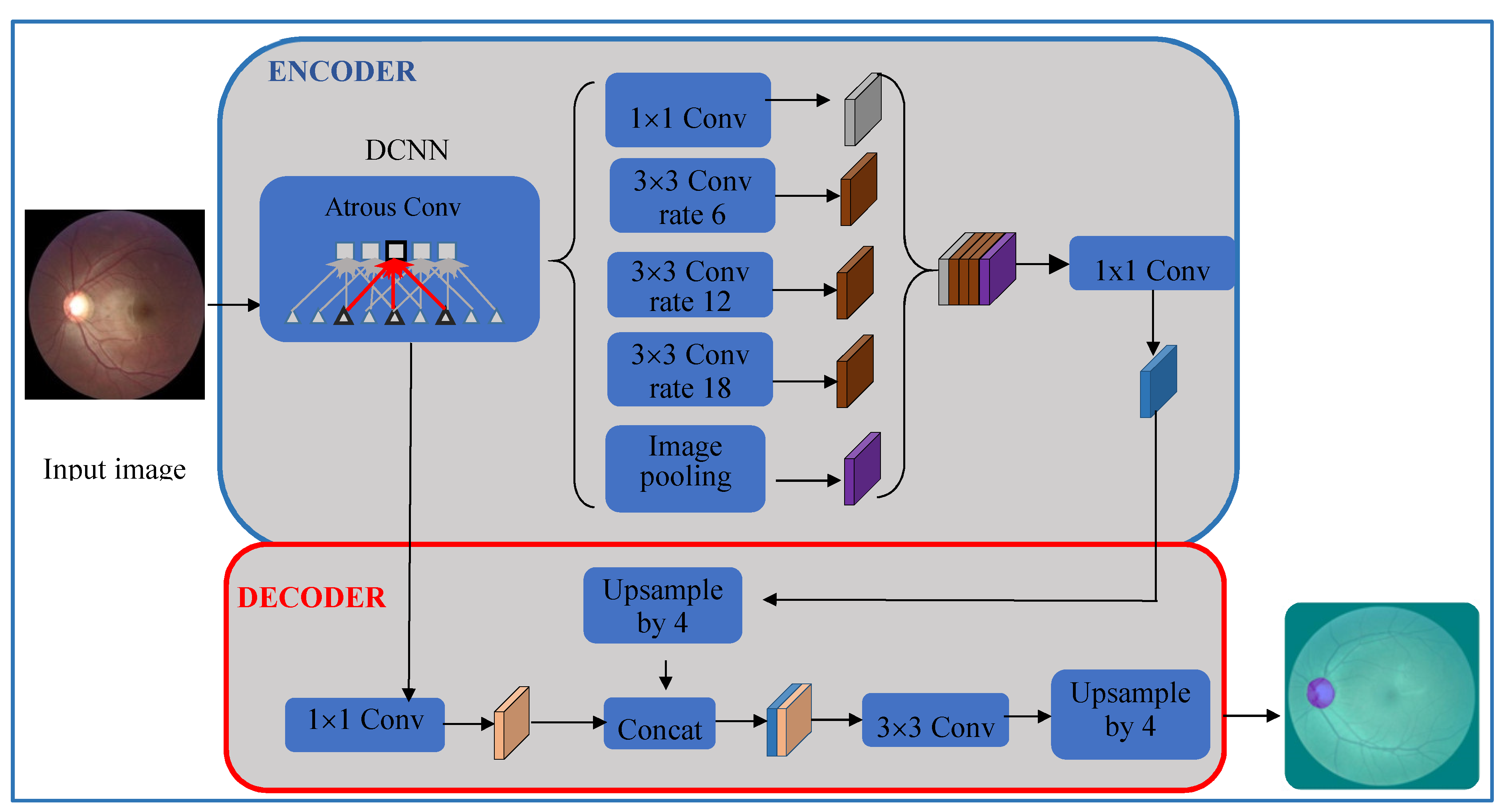
In this stage, the OD was segmented using DeepLabv3+ [29] and a bounding box was set, see Figure 3. DeepLabv3+ uses two phases: an encoder and a decoder. The encoder uses four parallel atrous convolutions at different rates to extract features. The extracted features were then concatenated, using average pooling, on the last feature map. To reduce the number of channels and obtain the best encoder features, 1 × 1 convolution was used. The decoder recovered the object boundaries encoded from CNNs model. The encoded features were first bilinearly upsampled by a factor of four and then concatenated with the corresponding low-level features. Since the corresponding low-level features usually contain a large number of channels, a 1 × 1 convolution filtered the important encoder features. Afterwards, a 3 × 3 convolution was used to refine the features followed by another bilinear upsampling by a factor of four. Five deep CNNs—ResNet18, ResNet50, XceptionNet, MobileNet and InceptionResNet—were used in the encoder phase and their segmentations were compared to find the best one for the encoder of DeepLabv3+. This generated the semantic mask for the OD region. OD extraction is illustrated in Figure 4. First, our segmentation formed a mask by labeling every pixel as OD or non-OD. The mask was laid over the original retinal image to extract the OD region. Finally, a bounding box cropped the OD region, which was input to the classification stage.

2.2. Classification of Normal and Glaucoma Retinal Images Using Deep CNNs

Here, we present three methods to apply deep CNNs to predict glaucoma in the retinal images:
(P1)
pretrained CNNs for transfer learning;
(P2)
pretrained deep CNNs as the feature extractors;
(P3)
an ensemble of methods, P1 and P2.

2.2.1. Transfer Learning Using Pretrained Deep CNNs (Method P1)

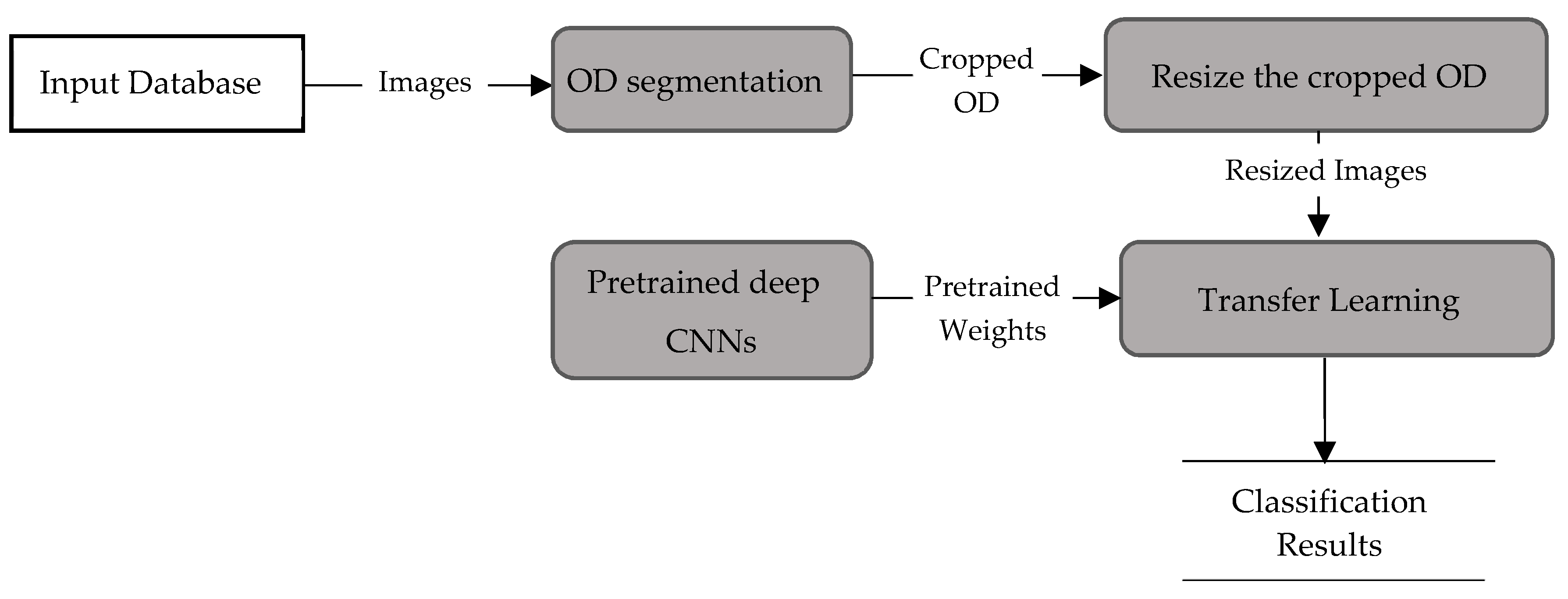
Method P1 used a transfer learning scheme based on pretrained deep CNNs. Eleven pretrained models—AlexNet [30], GoogleNet [31], InceptionV3 [32], XceptionNet [33], ResNet-50 [34], SqueezeNet [35], ShuffleNet [36], MobileNet [37], DenseNet [38], InceptionResNet [39] and NasNet-Large [40]—were evaluated. Table 2 lists the pretrained CNNs along with their specifications. The network depth presents the total number of layers from the input to the output of each model. DenseNet had the deepest depth with 201 layers, whereas AlexNet had only 8 layers. The inputs to all networks were RGB images. These models were pretrained on the ImageNet dataset for classification of thousands of natural objects. To adapt those models to predict glaucoma, a transfer learning technique was used, as shown in Figure 5. First, the OD was resized to the input size of each CNN model and the resized images were separately input to pretrained CNNs. The last fully connected layer of each model was replaced with the new layer. The new fully connected layer was trained and fine-tuned on the cropped OD images to classify between normal and glaucoma. Cross entropy loss was optimized during each iteration:
CE ( Y , Y Predict ) = c = 1 2 Y c log ( Y c Predict ) + ( 1 Y c ) log ( 1 Y c Predict )
where Y is the target vector and Y Predict is the predicted class vector: the vector elements are binary—0 represents normal and 1 represents glaucoma. Each CNN model was trained using the Adam optimizer [41] with default parameters: initial learning rate, α = 0.001, decay rate of gradient moving average = 0.9 and squared gradient moving average = 0.999.

2.2.2. Pretrained CNNs as Features Descriptors and SVM as Classifier (Method P2)

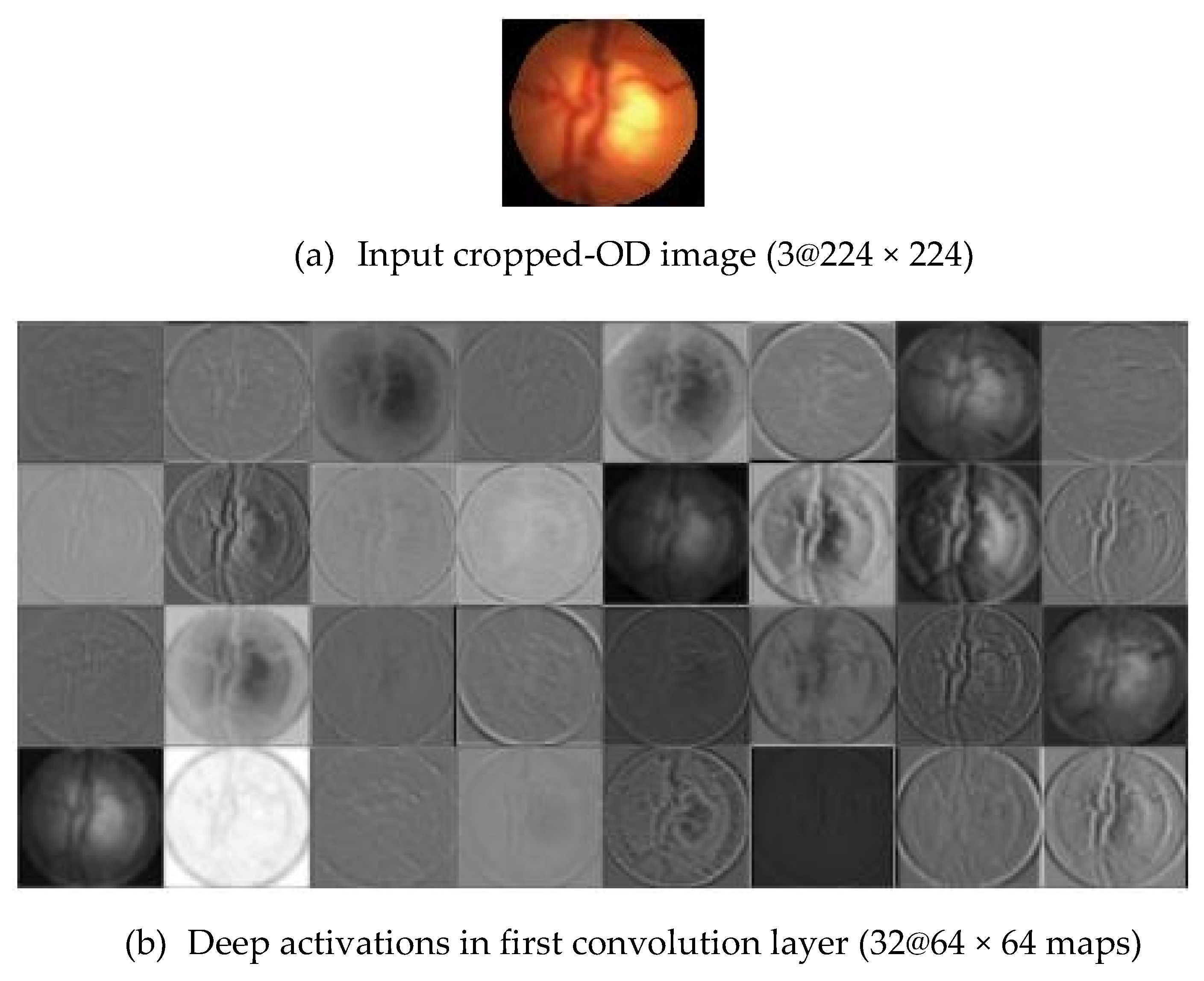
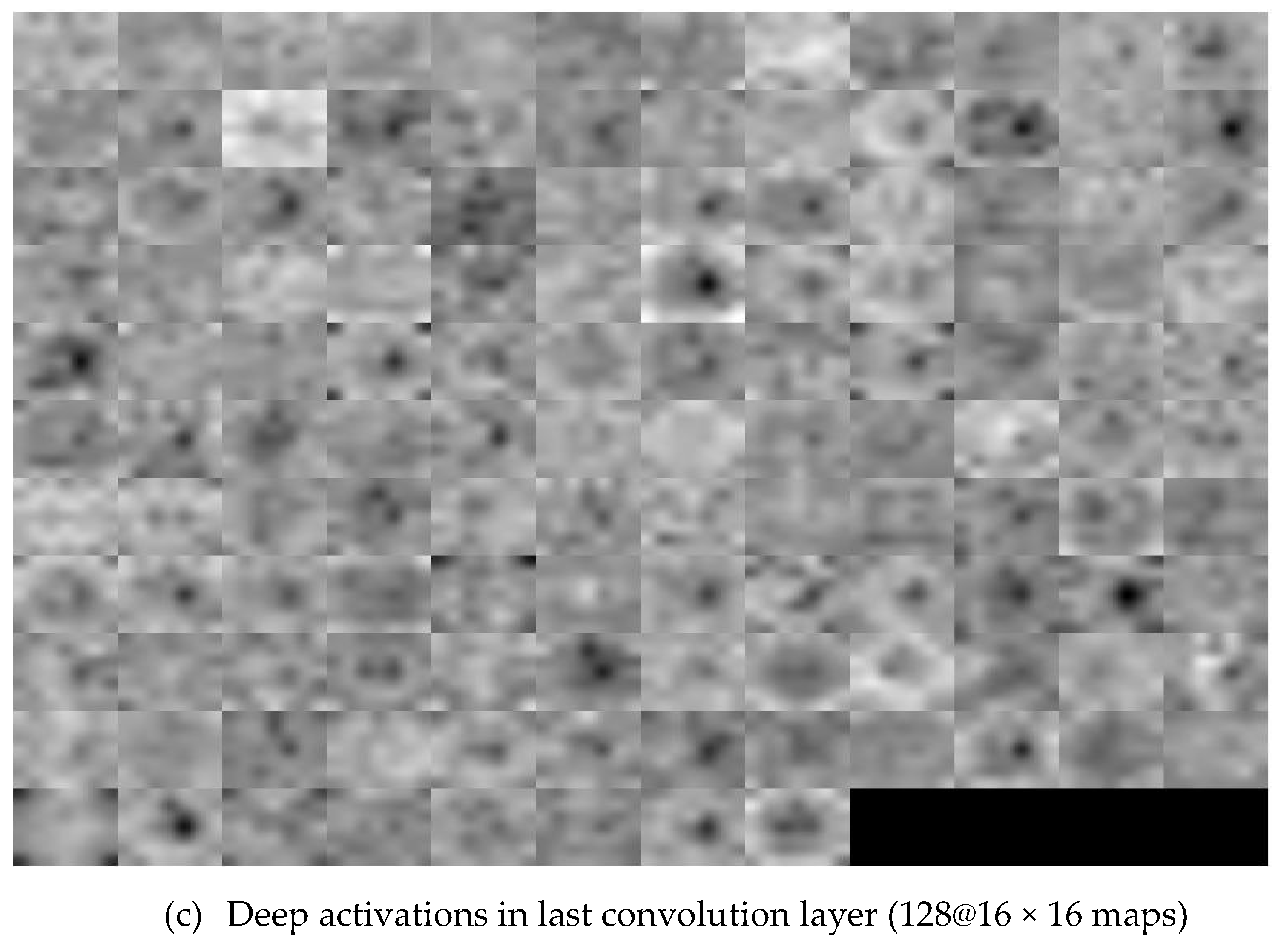
Method P2 used the same pre-trained CNNs, used in method P1, as the feature descriptors to extract the deep activated features, as shown in Figure 6. As in method P1, cropped OD regions were resized to the input size required by the CNNs, and then propagated in the network. The early convolutional layers of CNNs had a small receptive field and learnt small, low-level features. The deeper layers, towards the end of the CNNs, held larger receptive fields and learnt larger features. Figure 7 displays an example of activations (feature maps) of two convolution layers (the first: ‘conv2d-block1-1-conv’ and the last: ‘conv2d-block32-1-conv’) in DenseNet. These activation maps revealed the features that the CNN learnt. One can observe that channels in earlier layers learnt simple features, like color and edges, while channels in the deeper layers learnt complex features like blood vessels or the optic cup. Here, following Rokach [42], the fully connected layer and the last layer before classification, was flattened to retrieve the deep activated features. We extracted 1000 deep activated features from each CNNs and input them separately to the SVM classifier to identify a glaucoma. An SVM classifier aims to find an optimal decision hyperplane that maximizes the margin between normal and glaucoma data points. The number of training points is moderate, so an SVM classifier with Gaussian radial basis functions was used. Given the training data, D =   { ( x i , y i ) ,   i = 1 N } and y i { 1 , + 1 } , the general form of SVM classifier and the mapping function of the Gaussian kernel are defined in Equations (2) and (3):
min w , b , ξ 1 2 | | W | | 2 + C i ξ i 2   subject   to   y i ( W T X i + b )   1 ξ i , ξ i 0 ,   i
where C > 0 is the selected parameter and ξ is a set of slack variables.
K ( X , Y ) = e | | X Y | | 2 A
where K is a kernel function and A is a constant.

2.2.3. Ensemble Learning of Methods in P1 and P2

The basic idea of ensemble learning is similar to the real screening process in a hospital, when an ophthalmologist makes a glaucoma screening, the chance of a false diagnosis is given. When there is a doubt, the ophthalmologist asks other experts for more options. Similarly, our ensemble combines the predictions of multiple individual learners (individual ophthalmologists) into a consolidated prediction, reducing the generalization error. Predictions from ensemble CNNs were shown to be more accurate and effective than those based on an individual CNN [26,27]. Therefore, we built two ensemble classifiers– ensembles of the methods P1 and of the methods P2, as shown in Figure 8. The predictions of the ensemble classifiers were computed by averaging the predicted probability of each individual classifier. The predicted probability of ensemble classifier for an input image x is:
P ( y = j | x ) = exp [ n = 1 N P ^ n ( y = j | x ) ] exp [ l = 1 L n = 1 N P ^ n ( y = l | x ) ]
where n is each model, N is the number of models, L is the number classes and P ^ n ( y = j | x ) is the probability distribution.

3. Experimental Results

This study was experimented using Matlab 2019b in Window 10 and Nivida T1660Ti with core i7. We tested our work on 2787 retinal images from the five public databases: REFUGE, ACRIMA, ORIGA, RIM-ONE and DRISTI-GS1. REFUGE dataset contains 1200 retinal images captured using either Seiss Viscucam or Canon CR-2 from Chinese patients. The images were centered on both macular and OD visible, for the purpose of examining optical head nerve damage and retinal nerve fiber layer defects. The dataset contains pixel-wise annotations of OD and OC and classification labels of normal and glaucomatous marked by seven ophthalmologists. Poor quality images were discarded by the ophthalmologists during image labeling. The dataset was predefined into three subsets: training (400 images), validation (400 images), and testing (400 images), and each set contains an equal proportion of glaucomatous (10%) and non-glaucomatous (90%). ACRIMA dataset was created by the Ministerio de Economía y Competitividad of Spain for the classification of glaucomatous images. The dataset contained 309 normal and 396 glaucomatous images captured by Topcon TRC retinal camera with a 35° field of view (FOV). The images were taken from the eyes dilated and centered in OD. Only high-quality images were selected to avoid artefacts, noises and poor contrast. Two glaucoma experts manually labeled the images into either normal or glaucoma. ORIGA dataset is a part of SiMES dataset which was collected from 3280 Malay adults aged 40 to 80 and annotated by the trained professionals from Singapore Eye Research Institute. A total of 650 images were selected with the manual segmentation of OD and OC regions. It also provides CDR and labels for each image as glaucomatous or healthy. The RIM-ONE dataset was created for optic nerve head evaluation and glaucoma disease classification. It composed of 169 images which were captured and cited from three different hospitals in Spain (Hospital Universitario de Canarias, Hospital Clínico San Carlos and Hospital Universitario Miguel Servet) to guarantee the problems in image acquisition. All images are non-mydriatic retinal photographs captured with specific flash intensities. Five experts collaborated to annotate and label the retinal images into 3 classes: healthy, suspicious, and glaucoma. As suspicious case is out the scope of this study, we picked only 131 images (92 healthy and 39 glaucomatous images). DRISHTI-GS1 dataset was collected at Aravind eye hospital, Madurai and consists a total of 101 images (31 normal and 70 glaucomatous images). It is divided into 50 training and 51 testing images. All images were taken with the eyes dilated and centered in OD with 35° FOV. Poor quality images were discarded in terms of contrast, noise and position of OD. Four glaucoma experts with different clinical experiences examined and labeled each image into either normal or glaucoma. Table 3 summarizes the main characteristics of each dataset. All these datasets are collected for the purpose of optic nerve head assessment and glaucoma detection. The images in all datasets focus on OD region, whereas the images in REFUGE dataset were centered on both macula and OD visible. During the labeling process, only high-quality images were selected due to artefacts, noises, poor contrast and OD’s position, etc. As the images from different datasets were taken from different ethnicity by different devices and different FOV, we separately tested the proposed methods using each dataset.
Our method consists of two stages: OD segmentation and glaucoma classification. First, OD is detected and segregated from the full retinal images using DeepLabv3+ with five different backbone networks. Using the segmented OD, three deep learning-based methods were developed to identify glaucomatous images. For statistical evaluation of OD segmentation stage, only REFUGE dataset is used as it provided pixel-wise annotation of OD region. To evaluate the OD segmentation performance, we counted pixels matching the ground-truth maps. Figure 9 displays the overlap between the white OD mask (ground-truth) and our OD detection (pink mask). Based on the number of pixels overlap between the mask from OD detection and the ground truth mask, three evaluation metrics were computed: accuracy, dice coefficient, and Intersect over Union (IoU).
Accuracy = TP +   TN TP + TN + FP + FN
IoU = TP TP + FP + FN
Dice   coefficient   = 2 TP 2 TP + FP + FN
where
  • True Positive (TP) is the number of correctly prediction of OD pixels;
  • True Negative (TN) is the number of correctly detection of non-OD pixels;
  • False Positive (FP) is the number of wrongly detected of non-OD pixels as OD pixels;
  • False Negative (FN) is the number of wrongly identified of OD pixels as non-OD pixels.
Table 4 shows OD segmentation results using five different deep semantic algorithms. Combinations of DeepLabv3+ with ResNet18, ResNet50, XceptionNet, InceptionResNet and MobileNet models achieved comparable accuracy—between 99.64% and 99.72% with the average computational time 3.7 s per image. For the dice coefficient and IoU, the combination of DeepLabv3+ and MobileNet model achieved the best performance with dice coefficient of 91.73% and IoU of 84.89%. Therefore, the best-performing pair (a combination of DeepLabv3+ and MobileNet) is employed as the OD segmentation algorithm.
Once OD segmented, it is fed as input to the classification stage. Three proposed methods based on deep learning are applied to identify between non-glaucomatous and glaucomatous OD. We tested each method on all datasets individually to investigate their performance on different datasets. The performance of each method is evaluated and validated using two performance measures: accuracy and area under ROC curve. Table 5 demonstrates the experimental results obtained from the first proposal P1 using eleven different deep CNNs as the transfer learning models. The results showed that DenseNet model achieved the best performance for ACRIMA dataset with an accuracy of 99.53% and AUC of 99.98%, followed by MoblieNet and XceptionNet and achieved the similar best performance with MobileNet model for REFUGE dataset with the accuracy of 93.00% and AUC of 94.64% while MoblieNet model achieved the accuracy of 94.50% and AUC of 93.04%. MobileNet model achieved the best performance for ORIGA dataset with an accuracy of 80.51% and AUC of 81.54%, followed by InceptionResNet model which obtained the accuracy of 80.00% and AUC of 81.31%. For RIM-ONE dataset, SqueezeNet model achieved the best result with the accuracy of 97.37% and AUC of 100%, followed by DenseNet model with the accuracy of 94.74% and AUC of 99.04%. For DRISTI-GS1 dataset, ShuffleNet model is superior compared to other deep CNN models with an accuracy of 86.67%, but AlexNet model achieved the best performance in term of AUC with the result of 81.48%.
Table 6 shows the performance of the method P2 obtained from a SVM classifier using deep-activated features of eleven different pretrained CNNs across the datasets. Deep-activated features from DenseNet model provided the best performance for ACRIMA datasets with an accuracy of 96.23% and AUC of 98.75%, followed by the SqueezeNet model with the accuracy of 94.81% and AUC of 98.45%. For REFUGE dataset, DenseNet, ShuffleNet and ResNet-50 models achieved similar best performance, respectively with the accuracy of 93.50%, 93.75% and 94.75% and AUC of 93.94%, 92.24% and 90.66%. For DRISTI-GS1 dataset, InceptionResNet achieved the best results with the accuracy of 83.33% and AUC of 91.53% and achieved similar best performance with InceptionV3 model for ORIGA dataset with the accuracy of 78.46% and AUC of 82.06%, while InceptionV3 achieved the accuracy of 78.97% and AUC of 81.39%. For RIM-ONE dataset, ShuffleNet model achieved the best performance with an accuracy of 89.47% and AUC of 97.44%, followed by MoblieNet model which obtained the accuracy of 86.84% and AUC of 94.23%.
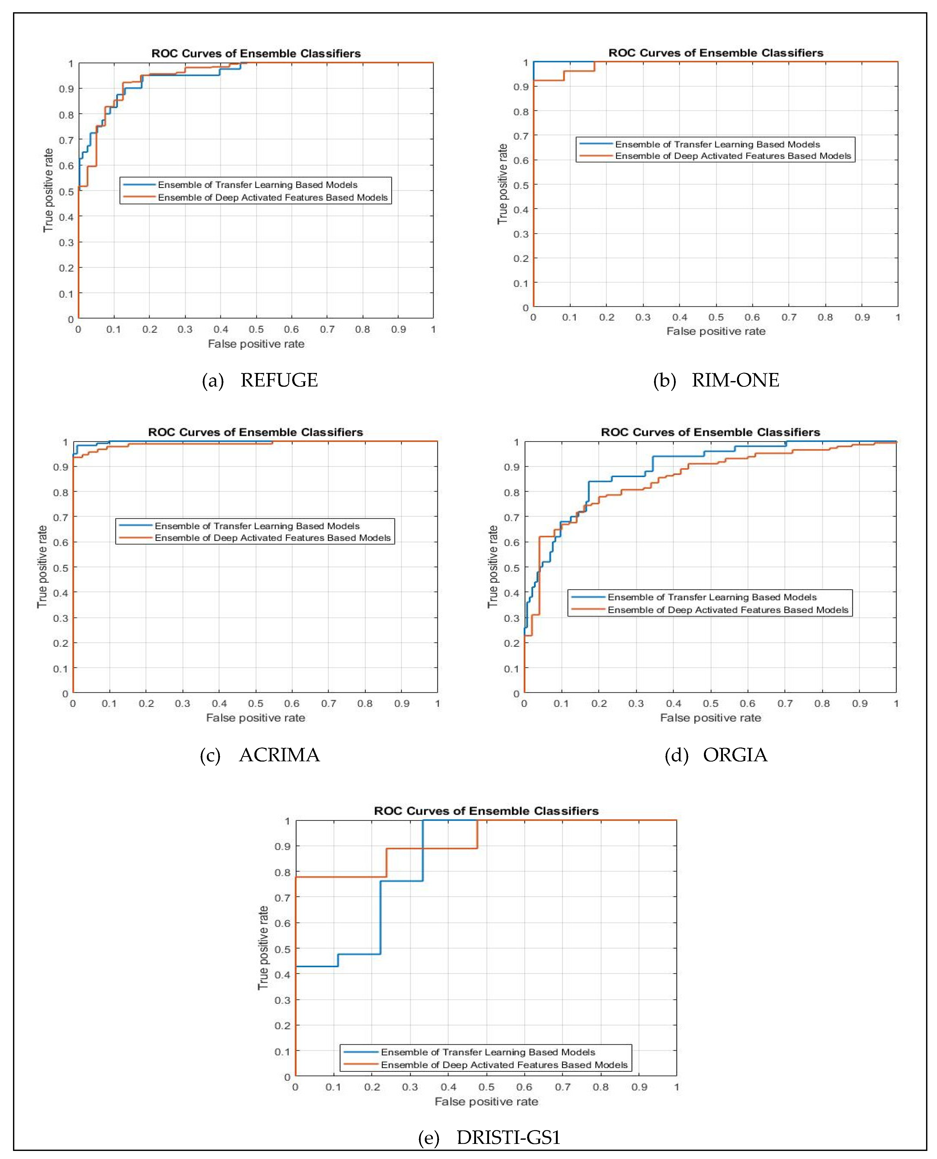
Table 7 illustrates the performance of the ensemble built by combining methods in each proposal P1 and P2 using average probabilities. The experimental results indicated that E(P1) achieved the best performance for RIM-ONE, ACRIMA and ORIGA datasets with the accuracy of 97.37%, 99.53% and 83.59% and AUCs of 100%, 99.98% and 88.86%, respectively, and achieved similar best performance with E(P2) for REFUGE dataset with the accuracy of 95.50% and AUC of 95.10%, while E(P2) achieved the accuracy of 95.75% and AUC of 94.32%. The E(P2) achieved the best performance for DRISTI-GS1 dataset with the accuracy of 90.00% and AUC of 92.06%. Table 5, Table 6 and Table 7 show that the results obtained from ACRIMA dataset are superior compared to other datasets and the ensemble methods, E(P1) and E(P2), perform well to find the optimal combination of the predictions managed to achieve the best performance for all five datasets with the average computational time 40 s and 53 s per image, respectively for E(P1) and E(P2).
To evaluate ensemble methods E(P1) and E(P2) visually, we plotted ROC curves based on the relationship of the true positive and false positive rates for all five different datasets as demonstrated in Figure 10. The graphs visualize that the closer such a curve is to the top-left corner, the better results of the methods are. As an example of using ACRIMA dataset, the AUC value of E(P1) achieve better than as of E(P2) is the same results as of ROC curves illustrated in Figure 10b, the blue curve E(P1) is closer to the top-left corner comparing to that of orange curve E(P2). The same way for other four datasets as showed in Table 5, ROC curves of E(P1) are closer to the top-left corner comparing to that of E(P2) for REFUGE, RIM-ONE and ORIGA datasets, while ROC curve of E(P2) is closer to the top-left corner comparing to that of E(P1) for DRISTI-GS1 dataset.

4. Discussion

An automated glaucoma diagnosis system is an essential task to save people’s vision due to its value in assisting the ophthalmologists to screen the glaucoma disease in a faster and inexpensive way. However, the lack of a common standard for comparison makes the evaluated result is not necessarily best comparing to the previous methods due to the use of different databases. To ease the validation criteria, we experiment several methods in each dataset separately and compare all results of our proposed methods in this study as well as compare with the common works in the literature which used the same experimental data. 2787 retinal images from five datasets are used separately to evaluate the performance of the proposed methods. The results indicate that the top score of methods in P1 achieves better performance for REFUGE, RIM-ONE and ACRIMA datasets comparing with the top score of methods in P2, while the top score of methods in P2 is superior compared to the top score of methods in P1 for DRISTI-GS1 dataset. However, the top score of both methods achieves the similar performance using ORIGA dataset. To improve the performance of glaucoma detection, the ensemble method is applied. The result indicates that E(P1) and E(P2) are superior comparing to the top score of methods in P1 and P2, respectively for all five datasets. For overall, E(P1) achieves the best performance for RIM-ONE, ACRIMA and ORIGA datasets and achieve similar best performance with E(P2) for REFUGE dataset while E(P2) achieves the best performance for DRISTI-GS1 dataset. In addition, we also compare our results with the previous works as reported in Table 8. The results indicate that our methods, both E(P1) and E(P2), achieve better results comparing to the conventional methods for RIM-ONE, ORIGA, DRISTI-GS1 and ACRIMA datasets with the accuracy of 97.37%, 90%, 86.84% and 99.53%, and AUC of 100%, 92.06%, 91.67% and 99.98%, respectively, and achieve the comparable results with CUHKMED, the top team in REFUGE challenging using REFUGE dataset with the accuracy of 95.59% and AUC of 95.10%.
From the above study, we found that the studies in [15,19,20] used simpler machine learning to classify the features from the cropped OD images for glaucoma classification and achieved the accuracy of 76.77%, 81.32%, and 76.90%, respectively on different datasets. The obtained results were not really promising. Deep CNN models were applied in [6,21,22,23] and they achieved better performance. However, those papers applied an individual CNN architecture using one or two datasets. It cannot be sure that their best CNN model will be good for another dataset. To address this matter, here we performed a comparative study from eleven CNN models using transfer learning technique in P1 and deep feature extraction technique along with SVM classifier P2 using Five datasets. Orlando et al. [5] presented the ensemble of CNN models and they achieved very good results using REFUGE dataset. Nevertheless, they used only a few CNN architectures with similar structure, four ResNet models, which did not efficiently explore the other potential features. In our study, we developed the ensemble of diverse CNN models using eleven CNN models with different architecture and each of them with different learning perspective. As all the methods presented in our study are tested and validated on five online available datasets, we believe that the obtained results will be valuable for future studies.
Although the obtained results are promising, there are still rooms for improvement and limitations to be alleviated. One fundamental limitation rises from the datasets when trying to generalize. We found that the available datasets are different in the way they are captured from different ethics using different devices, the labeling criteria and the quality of the image. Since our study separately tested each dataset, each algorithm is trained on the dataset with same devices, race and similar appearance. One dataset rarely contains diversity of images from different device, race. Ethnicities manifest differently in retinal image due to changes in the pigment of the fundus. Therefore, the proposed model performed differently on different datasets. By using the same dataset, it cannot be sure that the obtained best performing models can be used to a different population and achieve the same outcomes without retraining. Another issue is that the datasets used here contained only high-quality images. In real screening setting, it is expected to encounter low quality images and images with affects and noises. Therefore, a representative screening dataset with co- morbidities, diverse ethnicities, ages and genders and low-quality images with acquisition artifacts, is in urgent need.
Moreover, we can observe from our results that CNN models performed differently on the underlying data across the datasets. It may occur due to two different patterns; the dataset size and the imbalance data between glaucomatous and non-glaucomatous images. Although REFUGE, ORIGA and ACRIMA datasets are large enough for generalization of deep learning methods, RIMONE and DRISTI-GSI are quite small. Therefore, the models trained on these small datasets maybe over fitted. Therefore, we intend to enlarge these datasets to validate the robustness of the evaluated methods and even to build a customized deep learning method. Enlarging the datasets can be done by using image augmentation methods or using generative adversarial networks (GAN). Regarding imbalance data, except ACIRMA dataset, the rest datasets are heavily class-imbalanced where the number of glaucomatous are tiny and the number of non-glaucomatous are abundant. The class-imbalanced data can cause the classification bias in the deep learning algorithms which likely to favor to major class. This problem can be addressed by balancing the datasets in two different ways: adding more images to minor groups or using data sampling methods, and it remains as the future works.
Furthermore, in this study, we used only deep learning methods to make the classification decision between glaucomatous and non-glaucomatous images. The main measurements used in previous studies such as CDR and measurement of OD and OC are excluded. Incorporating deep learning methods with these OD and OC related measurements may improve the classification accuracy of glaucomatous images. To measure CDR, we need to segment both OD and OC region. As our current segmentation method is designed for OD segmentation only, we need to redesign the proposed segmentation method to segment both OD and OC simultaneously.
Finally, it is to highlight the disease screening scheme. This study aims for binary classification of normal and glaucomatous image. In this future, it would be more beneficial to develop an automated screening system for all possible eye disease such as diabetic retinopathy, glaucoma, myopia, age related macular degeneration, vascularization, etc., which can be examined using retinal images.

5. Conclusions

This study presents an automatic primary screening of glaucoma based on quantitative analysis of fundus images to assist ophthalmologists for glaucoma disease detection in a faster and inexpensive way. The proposed method consists of two main processing steps. OD segmentation is experimented on five different deep semantic algorithms then the extracted features from the cropped OD region are used as an input to training a classifier for prophesying the presence of glaucoma in the testing images. Three proposals are presented to classify glaucomatous images; (P1) pre-trained CNNs using transfer learning, (P2) pretrained CNNs features using SVM classifiers and (P3) the ensemble of methods in P1 and P2. The methods are evaluated on five datasets containing 2787 retinal images, namely REFUGE, ACRIMA, ORIGA, RIM-ONE and DRISHTI-GS1. The best option for OD segmentation was the combination of DeepLabv3+ and MobileNet, which achieved an accuracy of 99.7%, a dice coefficient of 91.73% and IoU of 84.89%. For glaucoma classification, the ensemble of the proposed methods performs well to find the best performance comparing to the conventional methods for RIM-ONE, ORIGA, DRISTI-GS1 and ACRIMA datasets with the accuracy of 97.37%, 90%, 86.84% and 99.53% and AUC of 100%, 92.06%, 91.67% and 99.98%, respectively, and achieve comparable result with CUHKMED, the top team in REFUGE challenging using REFUGE dataset with the accuracy of 95.59% and AUC of 95.10%.

Author Contributions

S.S., N.M., K.H. and K.Y.W. conceived this research study. S.S. and K.Y.W. implemented the experiments, curated the simulation and data analysis and drafted the study. All authors have read and agreed to the published version of the manuscript.

Funding

This research work was funded by King Mongkut’s Institute of Technology Ladkrabang, Grant Number KREF146204.

Conflicts of Interest

The authors declare no conflicts of interest.

References

  1. World Health Organization. Global Report on Vision. World Health Organization. 2019. Available online: http://www.who.int/publications-detail/world-report-on-vision (accessed on 28 February 2020).
  2. Gupta, N.; Aung, T.; Congdon, N.; Lerner, F.; Dada, T.; Olawoye, S.; Resnikoff, S.; Wang, N.; Wormald, R. International Council of Ophthalmology Guidelines for Glaucoma Eye Care; International Council of Ophthalmology: San Francisco, CA, USA, 2016. [Google Scholar]
  3. Fu, H.; Cheng, J.; Xu, Y.; Zhang, C.; Wong, D.W.K.; Liu, J.; Cao, X. Disc-aware ensemble network for glaucoma screening from fundus image. IEEE Trans. Med. Imaging 2018, 37, 2493–2501. [Google Scholar] [CrossRef] [PubMed] [Green Version]
  4. Lundy, D.C.; Choplin, N.T. Atlas of Glaucoma; Informa: London, UK, 2007. [Google Scholar]
  5. Orlando, J.I.; Fu, H.; Breda, J.B.; van Keer, K.; Bathula, D.R.; Diaz-Pinto, A.; Fang, R.; Heng, P.A.; Kim, J.; Lee, J.; et al. REFUGE Challenge: A unified framework for evaluating automated methods for glaucoma assessment from fundus photographs. Med Image Anal. 2020, 59, 101570. [Google Scholar] [CrossRef]
  6. Diaz-Pinto, A.; Morales, S.; Naranjo, V.; Köhler, T.; Mossi, J.M.; Navea, A. CNNs for automatic glaucoma assessment using fundus images: An extensive validation. Biomed. Eng. Online 2019, 18, 29. [Google Scholar] [CrossRef] [PubMed] [Green Version]
  7. Zhang, Z.; Yin, F.S.; Liu, J.; Wong, W.K.; Tan, N.M.; Lee, B.H.; Cheng, J.; Wong, T.Y. Origa-light: An online retinal fundus image database for glaucoma analysis and research. In Proceedings of the 2010 Annual International Conference of the IEEE Engineering in Medicine and Biology, Buenos Aires, Argentina, 31 August–4 September 2010; pp. 3065–3068. [Google Scholar]
  8. Fumero, F.; Alayón, S.; Sanchez, J.L.; Sigut, J.; Gonzalez-Hernandez, M. RIM-ONE: An open retinal image database for optic nerve evaluation. In Proceedings of the 2011 24th International Symposium on Computer-Based Medical Systems (CBMS), Bristol, UK, 27–30 June 2011; pp. 1–6. [Google Scholar] [CrossRef]
  9. Sivaswamy, J.; Krishnadas, S.R.; Joshi, G.D.; Jain, M.; Tabish, A.U.S. Drishti-gs: Retinal image dataset for optic nerve head (onh) segmentation. In Proceedings of the 2014 IEEE 11th International Symposium on Biomedical Imaging (ISBI), Beijing, China, 29 April–2 May 2014; pp. 53–56. [Google Scholar] [CrossRef] [Green Version]
  10. Budai, A.; Bock, R.; Maier, A.; Hornegger, J.; Michelson, G. Robust vessel segmentation in fundus images. Int. J. Biomed. Imaging 2013, 2013, 154860. [Google Scholar] [CrossRef] [Green Version]
  11. Foong, A.W.; Saw, S.M.; Loo, J.L.; Shen, S.; Loon, S.C.; Rosman, M.; Aung, T.; Tan, D.T.; Tai, E.S.; Wong, T.Y. Rationale and methodology for a population-based study of eye diseases in Malay people: The Singapore Malay eye study (SiMES). Ophthalmic Epidemiol. 2007, 14, 25–35. [Google Scholar] [CrossRef]
  12. Sng, C.C.; Foo, L.L.; Cheng, C.Y.; Allen, J.C., Jr.; He, M.; Krishnaswamy, G.; Nongpiur, M.E.; Friedman, D.S.; Wong, T.Y.; Aung, T. Determinants of anterior chamber depth: The Singapore Chinese Eye Study. Ophthalmology 2012, 119, 1143–1150. [Google Scholar] [CrossRef]
  13. Pan, C.W.; Wong, T.Y.; Chang, L.; Lin, X.Y.; Lavanya, R.; Zheng, Y.F.; Kok, Y.O.; Wu, R.Y.; Aung, T.; Saw, S.M. Ocular biometry in an urban Indian population: The Singapore Indian Eye Study (SINDI). Investig. Ophthalmol. Vis. Sci. 2011, 52, 6636–6642. [Google Scholar] [CrossRef] [Green Version]
  14. Cheng, J.; Yin, F.; Wong, D.W.K.; Tao, D.; Liu, J. Sparse dissimilarity-constrained coding for glaucoma screening. IEEE Trans. Biomed. Eng. 2015, 62, 1395–1403. [Google Scholar] [CrossRef]
  15. Chakravarty, A.; Sivaswamy, J. Glaucoma classification with a fusion of segmentation and image-based features. In Proceedings of the 2016 IEEE 13th International Symposium on Biomedical Imaging (ISBI), Prague, Czech Republic, 13–16 April 2016; pp. 689–692. [Google Scholar]
  16. Karkuzhali, S.; Manimegalai, D. Computational intelligence-based decision support system for glaucoma detection. Biomed. Res. 2017, 28, 976–1683. [Google Scholar]
  17. Mohamed, N.A.; Zulkifley, M.A.; Zaki, W.M.D.W.; Hussain, A. An automated glaucoma screening system using cup-to-disc ratio via Simple Linear Iterative Clustering superpixel approach. Biomed. Signal Process. Control 2019, 53, 101454. [Google Scholar] [CrossRef]
  18. Selvathi, D.; Prakash, N.B.; Gomathi, V.; Hemalakshmi, G.R. Fundus Image Classification Using Wavelet Based Features in Detection of Glaucoma. Biomed. Pharmacol. J. 2018, 11, 795–805. [Google Scholar] [CrossRef]
  19. Maheshwari, S.; Pachori, R.B.; Acharya, U.R. Automated diagnosis of glaucoma using empirical wavelet transform and correntropy features extracted from fundus images. IEEE J. Biomed. Health Inform. 2016, 21, 803–813. [Google Scholar] [CrossRef]
  20. Guo, F.; Mai, Y.; Zhao, X.; Duan, X.; Fan, Z.; Zou, B. and Xie, B. Yanbao: A mobile app using the measurement of clinical parameters for glaucoma screening. IEEE Access 2018, 6, 77414–77428. [Google Scholar] [CrossRef]
  21. Bajwa, M.N.; Malik, M.I.; Siddiqui, S.A.; Dengel, A.; Shafait, F.; Neumeier, W.; Ahmed, S. Two-stage framework for optic disc localization and glaucoma classification in retinal fundus images using deep learning. BMC Med. Inform. Decis. Mak. 2019, 19, 136. [Google Scholar]
  22. Gómez-Valverde, J.J.; Antón, A.; Fatti, G.; Liefers, B.; Herranz, A.; Santos, A.; Sánchez, C.I.; Ledesma-Carbayo, M.J. Automatic glaucoma classification using color fundus images based on convolutional neural networks and transfer learning. Biomed. Opt. Express 2019, 10, 892–913. [Google Scholar] [CrossRef] [Green Version]
  23. Orlando, J.I.; Prokofyeva, E.; del Fresno, M.; Blaschko, M.B. Convolutional neural network transfer for automated glaucoma identification. SPIE: International Society for Optics and Photonics. In Proceedings of the 12th International Symposium on Medical Information Processing and Analysis, Tandil, Argentina, 26 January 2017; Volume 10160, p. 101600U. [Google Scholar]
  24. Asaoka, R.; Tanito, M.; Shibata, N.; Mitsuhashi, K.; Nakahara, K.; Fujino, Y.; Matsuura, M.; Murata, H.; Tokumo, K.; Kiuchi, Y. Validation of a deep learning model to screen for glaucoma using images from different fundus cameras and data augmentation. Ophthalmol. Glaucoma 2019, 2, 224–231. [Google Scholar] [CrossRef]
  25. Juneja, M.; Singh, S.; Agarwal, N.; Bali, S.; Gupta, S.; Thakur, N.; Jindal, P. Automated detection of Glaucoma using deep learning convolution network (G-net). Multimed. Tools Appl. 2020, 79, 15531–15553. [Google Scholar] [CrossRef]
  26. Win, K.Y.; Maneerat, N.; Hamamoto, K.; Syna, S. A cascade of encoder-decoder with atrous separable convolution and ensemble deep convolutional neural networks for Tuberculosis detection. IEEE Access 2020. under review. [Google Scholar]
  27. Karim, M.R.; Rahman, A.; Jares, J.B.; Decker, S.; Beyan, O. A snapshot neural ensemble method for cancer-type prediction based on copy number variations. Neural Comput. Appl. 2019, 1–19. [Google Scholar] [CrossRef] [Green Version]
  28. Tiulpin, A.; Thevenot, J.; Rahtu, E.; Lehenkari, P.; Saarakkala, S. Automatic knee osteoarthritis diagnosis from plain radiographs: A deep learning-based approach. Sci. Rep. 2018, 8, 1–10. [Google Scholar] [CrossRef]
  29. Chen, L.C.; Zhu, Y.; Papandreou, G.; Schroff, F.; Adam, H. Encoder-decoder with atrous separable convolution for semantic image segmentation. In Proceedings of the Springer on European Conference on Computer Vision (ECCV), Munich, Germany, 8–14 September 2018; pp. 801–818. [Google Scholar]
  30. Krizhevsky, A.; Sutskever, I.; Hinton, G.E. Imagenet classification with deep convolutional neural networks. In Proceedings of the Advances in Neural Information Processing Systems, San Francisco, CA, USA, 3–8 December 2012; pp. 1097–1105. [Google Scholar]
  31. Szegedy, C.; Liu, W.; Jia, Y.; Sermanet, P.; Reed, S.; Anguelov, D.; Erhan, D.; Vanhoucke, V.; Rabinovich, A. Going deeper with convolutions. In Proceedings of the IEEE Conference on Computer Vision and Pattern Recognition, Boston, MA, USA, 7–12 June 2015; pp. 1–9. [Google Scholar]
  32. Szegedy, C.; Vanhoucke, V.; Ioffe, S.; Shlens, J.; Wojna, Z. Rethinking the inception architecture for computer vision. In Proceedings of the IEEE Conference on Computer Vision and Pattern Recognition, Las Vegas, NV, USA, 27–30 June 2016; pp. 2818–2826. [Google Scholar]
  33. Chollet, F. Xception: Deep learning with depthwise separable convolutions. In Proceedings of the IEEE Conference on Computer Vision and Pattern Recognition, Honolulu, HI, USA, 21–26 July 2017; pp. 1251–1258. [Google Scholar]
  34. He, K.; Zhang, X.; Ren, S.; Sun, J. Deep residual learning for image recognition. In Proceedings of the IEEE Conference on Computer vision and Pattern Recognition, Las Vegas, NV, USA, 27–30 June 2016; pp. 770–778. [Google Scholar]
  35. Iandola, F.N.; Han, S.; Moskewicz, M.W.; Ashraf, K.; Dally, W.J.; Keutzer, K. SqueezeNet: AlexNet-level accuracy with 50x fewer parameters and < 0.5 MB model size. arXiv 2016, arXiv:1602.07360. [Google Scholar]
  36. Zhang, X.; Zhou, X.; Lin, M.; Sun, J. Shufflenet: An extremely efficient convolutional neural network for mobile devices. In Proceedings of the IEEE Conference on Computer Vision and Pattern Recognition, Salt Lake City, UT, USA, 18–23 June 2018; pp. 6848–6856. [Google Scholar]
  37. Sandler, M.; Howard, A.; Zhu, M.; Zhmoginov, A.; Chen, L.C. Mobilenetv2: Inverted residuals and linear bottlenecks. In Proceedings of the IEEE Conference on Computer vision and Pattern Recognition, Salt Lake City, UT, USA, 18–23 June 2018; pp. 4510–45206. [Google Scholar]
  38. Huang, G.; Liu, Z.; Van Der Maaten, L.; Weinberger, K.Q. Densely connected convolutional networks. In Proceedings of the IEEE Conference on Computer Vision and Pattern Recognition, Honolulu, HI, USA, 21–26 July 2017; pp. 4700–4708. [Google Scholar]
  39. Szegedy, C.; Ioffe, S.; Vanhoucke, V.; Alemi, A.A. Inception-v4, inception-resnet and the impact of residual connections on learning. In Proceedings of the Thirty-First AAAI Conference on Artificial Intelligence, San Francisco, CA, USA, 4–9 February 2017; Volume 4, p. 12. [Google Scholar]
  40. Zoph, B.; Vasudevan, V.; Shlens, J.; Le, Q.V. Learning transferable architectures for scalable image recognition. In Proceedings of the IEEE Conference on Computer Vision and Pattern Recognition, Salt Lake City, UT, USA, 18–23 June 2018; pp. 8697–8710. [Google Scholar]
  41. Kingma, D.P.; Ba, J. Adam: A method for stochastic optimization. arXiv 2014, arXiv:1412.6980. [Google Scholar]
  42. Rokach, L. Ensemble-based classifiers. Artif. Intell. Rev. 2010, 33, 1–39. [Google Scholar] [CrossRef]
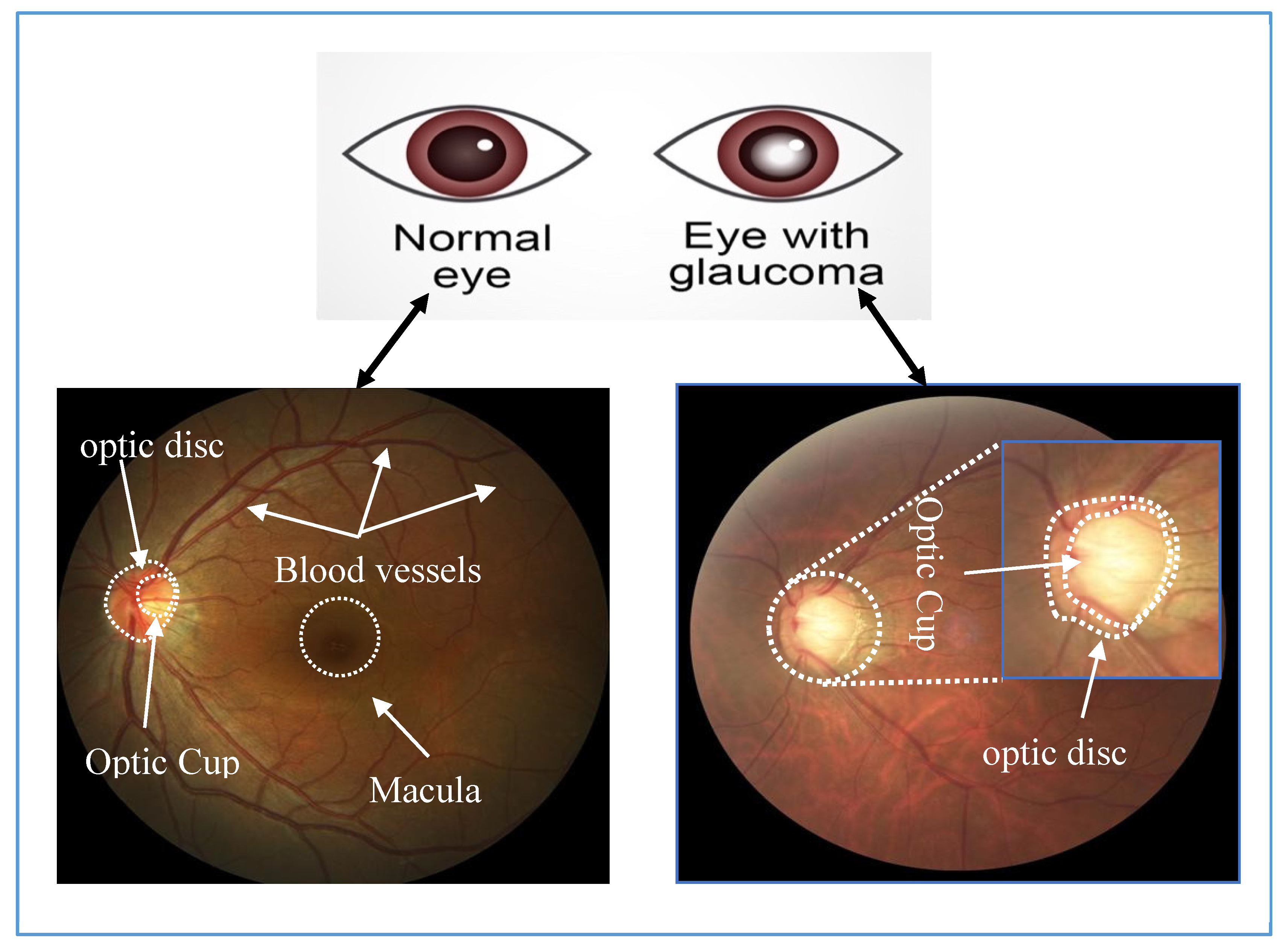
Figure 1. Images of a healthy retina (left) and one with glaucoma (right).
Applsci 10 04916 g001
Figure 2. Grading of glaucoma diseases: (a) healthy OD; (b) Mild Glaucoma; (c) Moderate Glaucoma and (d) severe glaucoma.
Applsci 10 04916 g002
Figure 3. Block diagram for optic disc (OD) detection using DeepLabv3+.
Applsci 10 04916 g003
Figure 4. Retrieving OD regions from the full retinal image using DeepLabv3+ and cropping to the bounding box.
Applsci 10 04916 g004
Figure 5. Data flow in method P1.
Applsci 10 04916 g005
Figure 6. Data flow for method P2.
Applsci 10 04916 g006
Figure 7. Visualization of the feature maps for two convolutional layers: (a) Input Cropped-OD image; (b) conv1 and (c) conv32 generated by DenseNet.
Applsci 10 04916 g007aApplsci 10 04916 g007b
Figure 8. Diagram showing ensemble of methods in P1 and P2.
Applsci 10 04916 g008
Figure 9. Pixel overlaps between our OD detection (pink masks) and the white ground truth mask.
Applsci 10 04916 g009
Figure 10. ROC curves of ensemble methods using five different datasets (a) REFUGE, (b) RIM-ONE, (c) ACRIMA, (d) ORIGA and (e) DRISTI-GS1.
Applsci 10 04916 g010
Table 1. Datasets for glaucoma detection.
DatasetNumber of ImagesGround Truth InformationSourceAvail
NormGlauTotal
REFUGE10801201200Pixel-wise annotations of OD and OC
Localization mask of Fovea
Classification labels of normal and glaucomatous
Orlando et al. [5]Online
ACRIMA309396705Classification labels of normal and glaucomatousDiaz-Pinto et al. [6]Online
ORIGA482168650Segmentation masks of OD and OC
Classification labels of normal and glaucomatous
Zhang et al. [7]Online
RIMONE9239131Manual segmentation masks of OD
Classification labels of normal and glaucomatous
Fumero et al. [8]Online
DRISHTI-GS13170101Manual segmentation masks of optic nerve head for 50 training images
Classification labels of normal and glaucomatous
Sivaswamy et al. [9]Online
HRF15
* DR 15
1545Segmentation masks of field of view (FOV), blood vessels and OD
Classification Labels of Normal, DR and Glaucomatous
Budai et al. [10]Online
SiMES482168650Classification labels of normal and glaucomatousFoong et al. [11]Private
SCES1630461676Classification labels of normal and glaucomatousSng et al. [12]Private
SiNDI56701135783Classification labels of normal and glaucomatousFu et al. [13]Private
Note: DR—diabetic retinopathy; Norm—normal; Glau—glaucoma; Avail—available.
Table 2. Pretrained convolutional neural networks (CNNs) and their properties.
NetworkDepthSize (MB)Parameters (×106)Image Input Size
AlexNet822761.0227 × 227
GoogleNet22277.0224 × 224
InceptionV3488923.9299 × 299
XceptionNet718522.9299 × 299
Resnet-10110116744.6224 × 224
ShuffleNet506.31.4224 × 224
SqueezeNet184.61.24227 × 227
MobileNet53133.5224 × 224
InceptionResNet16420955.9299 × 299
DenseNet2017720.0224 × 224
NasNet-Large*36088.9331 × 331
* NasNet—large does not consist of linear sequence of modules.
Table 3. The datasets for glaucoma detection task.
DatasetsNo. of ImagesImage Acquisition
CameraFOVResolutionEthnicityFocus
REFUGE1200Train: Zeiss Visucam 500JPEG 2124 × 2056ChineseCenter macula and OD visible
Validation/Testing: Canon CR-2JPEG 1634 × 1634
ACRIMA705Topcon TRC35°JPEG 2048 × 1536SpanishOD
ORIGA650JPEG 3072 × 2048MalayOD
RIM–ONE131Kowa WX 3D34°JPEG 2144 × 1424SpanishOD
DRISHTI–GS1101NM/FA30°PNG 2896 × 1944IndianOD
Total2787
Table 4. Statistical performance of various deep semantic algorithms for two classes segmentation between OD and non-OD.
MethodsPerformance Measures
AccuracyDice CoefficientIoU
DeepLabv3+ + ResNet1899.70%90.95%83.56%
DeepLabv3+ + ResNet5099.64%88.78%80.26%
DeepLabv3+ + XceptionNet99.71%91.39%84.48%
DeepLabv3+ + InceptionResNet99.72%91.29%84.21%
DeepLabv3+ + MobileNet99.70%91.73%84.89%
Table 5. P1: Transfer learning using eleven pretrained networks for glaucoma classification.
Pretrained Deep CNNsPerformance Measures
REFUGERIM-ONEACRIMAORGIADRISTI-GS1
ACC (%)AUC (%)ACC (%)AUC (%)ACC (%)AUC (%)ACC (%)AUC (%)ACC (%)AUC (%)
AlexNet90.0081.6974.8769.2196.2399.8568.4259.6270.0081.48
GoogleNet92.5088.6994.7491.0391.5196.4971.7977.0370.0079.89
InceptionV390.2587.2671.0576.9293.8799.3675.3876.8670.0065.08
XceptionNet89.0085.2981.5888.1498.1199.8077.4481.6866.6766.67
ResNet-5093.5092.9792.1198.0895.7599.5675.9080.1973.3378.31
SqueezeNet91.0089.5897.3710095.7598.8478.4679.1756.6776.19
ShuffleNet93.2594.0992.1197.4496.2399.7572.3180.0486.6778.84
MobileNet94.5093.0492.1199.3698.5899.9680.5181.5476.6773.02
DenseNet93.0094.6494.7499.0499.5399.9877.4473.9273.3378.31
InceptionResNet92.2592.0868.4261.8696.2398.8480.0081.3170.0068.78
NasNet-Large92.7590.4486.8495.1996.2399.8573.8577.7270.0069.31
Table 6. P2: Deep activated features from eleven pretrained networks and SVM for glaucoma classification.
Deep Features DescriptorsPerformance Measures
REFUGERIM-ONEACRIMAORGIADRISTI-GS1
ACC (%)AUC (%)ACC (%)AUC (%)ACC (%)AUC (%)ACC (%)AUC (%)ACC (%)AUC (%)
AlexNet93.0088.0786.8492.6391.5195.4776.4180.4680.0079.89
GoogleNet93.7587.8184.2190.3890.5790.5774.8775.2370.0072.49
InceptionV392.2590.3163.1674.0495.2895.2878.9781.3973.3370.90
XceptionNet93.2590.2678.9581.0991.0494.9075.9076.1273.3368.78
ResNet-5094.7590.6681.5891.6793.4098.3975.3880.1270.0062.96
SqueezeNet92.0084.8381.5896.1594.8198.4578.4680.0680.0078.84
ShuffleNet93.7592.2489.4797.4492.4597.9974.3677.5686.6783.07
MobileNet92.7589.2586.8494.2392.9296.4877.4481.3076.6785.71
DenseNet93.5093.9484.2189.7496.2398.7578.4681.9270.0077.25
InceptionResNet92.0088.7878.9591.9992.4596.6378.4682.0683.3391.53
NasNet-Large93.2590.8186.8493.5991.0495.9274.8779.2383.3380.42
Table 7. P3: Ensemble of methods in P1 and P2 for glaucoma classification.
Ensemble LearnersPerformance Measures
REFUGERIM-ONEACRIMAORGIADRISTI-GS1
ACC (%)AUC (%)ACC (%)AUC (%)ACC (%)ACC (%)AUC (%)ACC (%)AUC (%)ACC (%)
Ensemble of P1 (E(P1))95.5995.1097.3710099.5399.9883.5988.8683.3385.19
Ensemble of P2 (E(P2))95.7594.3292.1199.0496.2399.0180.0085.2690.0092.06
Table 8. Performance of the proposed methods for glaucoma classification.
DatasetsPerformance Measures
RIM-ONEMaheshwari et al. (2016) [19]Gómez-Valverde et al. (2019) [22]Diaz-Pinto
et al. (2019) [6]
Proposed method
ACC = 81.32%Sen = 87.01%
Spe = 89.01%
AUC = 94%
ACC = 71.21%
AUC = 85.75%
E(P1)E(P2)
ACC = 97.37%
AUC = 100%
ACC = 92.11%
AUC = 99.04%
DRISTI-GS1Chakravarty et al. (2017) [15]Orlando et al. (2017) [23]Diaz-Pinto
et al. (2019) [6]
Proposed method
ACC = 76.77%
AUC = 78%
AUC = 76.26%ACC = 75.25%
AUC = 80.41%
E(P1)E(P2)
ACC = 83.33%
AUC = 85.19%
ACC = 90%
AUC = 92.06%
ORIGAGUO et al. (2018) [20]Bajwa et al. (2019) [21]Proposed method
ACC = 76.90%
AUC = 83.10%
Sen=71.17%
AUC=87.40%
E(P1)E(P2)
ACC = 83.59%
AUC = 88.86%
ACC = 80.00%
AUC = 85.26%
ACRIMADiaz-Pinto et al. (2019) [6]Proposed method
ACC = 70.21%
AUC = 76.78%
E(P1)E(P2)
ACC = 99.53%
AUC = 99.98%
ACC = 96.23%
AUC = 99.01%
REFUGEOrlando et al. (2020) [5]Proposed method
Sen = 97.52%
AUC = 98.85%
E(P1)E(P2)
ACC = 95.59%
AUC = 95.10%
ACC = 95.75%
AUC = 94.32%