Disturbance and Uncertainty Suppression Control for a Saucer-Shaped Unmanned Aerial Vehicle Based on Extended State Observer

Abstract

For saucer-shaped unmanned aerial vehicles with blended wing bodies (BWBs), un-modelled coupling effect uncertainty and external disturbance missing the matching conditions have always been the concerns. To solve this flight control problem, this research has proposed a composite backstepping controller incorporated with a finite-time convergent differentiator and a nonlinear extended state observer (ESO). More specifically, the differentiator is employed to obtain the derivatives of the virtual control laws in finite-time and therefore eliminate the inherent “explosion of term” problem in backstepping. By the effective real-time estimation of ESO without the peaking value problem, the total effect of internal uncertainties and external disturbances is compensated in the control law design, which can dispense with parameter identification and model approximation. Furthermore, based on Lyapunov theory, it is proved rigorously that all the signals of the resulting closed-loop systems are bounded. In the final part of this paper, simulation results are presented to validate the effectiveness of the proposed control scheme.

1. Introduction

In past decades, aircraft design has been changed radically in the aviation industry. As the conventional aircraft cannot meet our requirement for a higher lift-to-drag (L/D) ratio, higher payload carrying capacity and more excellent stealth effect, etc., lifting body/blended wing body (BWB) becomes a potential solution to bridge the gaps. A lifting body is an aerial vehicle that chiefly, even solely, produces lift in the body [1], which is always designed as a unique tailless single entity where the fuselage is merged with the wings. Since such aircrafts cancel the vertical tail and typical rudders, several kinds of innovative control effectors (ICEs) are introduced to improve the aerodynamic efficiency and manoeuvrability, such as leading-edge flaps (LEFs), split drag rudders (SDRs) and spoiler-slot-deflectors (SSDs) [2], etc. Motivated by the aforementioned design philosophy, more and more lifting bodies/BWBs such as M2-F3, HL-20, X-24B, BWB-450, etc. (see also in [3]) have been developed successively. The saucer-shaped unmanned aerial vehicle (UAV) studied in this paper is also derived from the same design concept.

However, BWB aircrafts suffer from disadvantages such as the high nonlinearity, strong interactions and coupling effects between control effectors (which is difficult for modelling) as well as serious parameter uncertainties. Moreover, during actual flight, the existence of gust wind and turbulence needs to be taken into consideration, which also brings challenges to controller design. Until now, abundant approaches have been proposed by worldwide researchers. Most of the approaches are related to advanced, nonlinear methodologies, such as nonlinear model predictive controller (NMPC) [4], trajectory linearization control (TLC) [5,6] and sliding mode control (SMC) [7], to name a few. An improved $H\infty$ robust controller is established to handle the coupling effects considering longitudinal turbulence in [8]. By addressing stability control in the presence of disturbances, a finite time convergence sliding mode control scheme is developed in the linear parameter-varying model of the aircraft [9]. However, the methods mentioned above are either inherently model-dependent with computational concerns or only insensitive to the matched disturbance. It is noted that both matched and mismatched disturbances/uncertainties should be considered for the flight control system design, as it is inevitable that the un-modelled coupling effect uncertainty and external disturbance would arise in different channels as the control input.

To estimate and suppress the mismatched disturbances/uncertainties, some effective techniques have been investigated including disturbance observer (DO)-based SMC method in [10,11], the Riccati approach combined with SMC in [12] and active disturbance rejection control (ADRC) in [13,14]. However, most of these approaches require that the disturbances $d(t)$ satisfy $\underset{x\to \infty }{\lim }\dot{d}(t)=0$, which is so-called “mismatched vanishing disturbances”, or the accurate expressions of the mismatched uncertain terms were assumed to be known in [13,14]. The backstepping technique is a powerful tool for nonlinear systematic design in the presence of mismatched uncertainties. Since the core of this method is to design a controller recursively by considering some of the state variables as “virtual controls” and by designing for their intermediate control laws, the “backward steps” can accommodate the uncertainties missing the matching conditions. A composite anti-disturbance controller [15] is synthesized by introducing disturbance estimations into the design of virtual control laws to compensate for mismatched disturbances with partial known information. Zhai et al. [16] proposed a new robust adaptive fuzzy control method by combining $H\infty$ theory with backstepping technique for a class of uncertain nonlinear systems with unstable dynamics and mismatched disturbances. However, the standard backstepping algorithm has the inherent disadvantage of an “explosion of terms” caused by the repeated differentiations of virtual controllers.

To eliminate the drawback of classical backstepping, dynamic surface control technique combined with adaptive neural networks [17] or fuzzy logic systems [18] were put forward for a class of uncertain nonlinear systems with external disturbances. On the other hand, the command filtered backstepping method [19,20] was investigated to alleviate the calculation burden, in which complex error compensation mechanism (ECM) should be designed to ensure control performance. Compared with the asymptotic control approach, the finite time control technique has the advantages of faster response, higher tracking precision and better disturbance-rejection ability. Jiang et al. [21] addressed a novel composite backstepping framework, where finite-time convergence property is guaranteed by introducing the fractional power functions of tracking errors and the finite-time filters of intermediate command signals. In [22], the first-order Levant differentiator has been applied to each step of the backstepping, which can approximate the derivative of the virtual control in finite-time.

In industrial applications, the extended state observer (ESO) technique has been attracting intensive attention, as it can simultaneously estimate the internal uncertainty (parameters or structure) and external disturbance in real time even in the absence of an accurate mathematical model of the system [23,24]. Successful applications include mechatronics systems [25], hydraulic system [26], quadrotors [27], autonomous driving [28], etc. Li et al. [29] firstly explored a generalized extended state observer (GESO) for multi-input–multi-output systems with nonintegral-chain form and mismatched disturbances/uncertainties. Guo et al. first conducted the theoretical analysis of nonlinear ESO in [30]. The study provided a rigorous proof of the convergence of high-gain nonlinear ESOs for one kind of nonlinear system with large uncertainty both from internal and external disturbances. Nevertheless, high observer gain will give rise to the peaking phenomenon, which may deteriorate transient performance.

According to the foregoing researches, a novel differentiator-based backstepping control scheme combined with a nonlinear ESO for a saucer-shaped BWB UAV subject to both matched and mismatched nonvanishing disturbances/uncertainties is proposed and carried out in this paper. Compared with the existing research, the main contribution of this paper is therefore threefold:

1. The problem of “explosion of terms” is eliminated by employing a finite-time-convergent second-order differentiator, which can not only precisely filter the virtual control command and obtain their differential signals but also guarantees the finite-time stable property.

2. To achieve the precise altitude controller design, a nonlinear ESO is proposed to estimate and compensate the total effect of parametric uncertainties, un-modelled dynamics and external disturbances in real time by viewing them as an extended state of the system. The nonlinear gain function alleviates the peaking value problem and improves observer performance.

3. A differentiator-based composite backstepping control framework integrated with the ESO technique is developed, along with a detailed stability analysis of the whole closed-loop structure. The proposed control scheme of the saucer-shaped BWB UAV fills in the gaps of related researches on aircrafts with innovative configurations.

In what follows, Section 2 will provide the mathematical model of the saucer-shaped UAV and the related problem description. In Section 3, the composite differentiator-based backstepping controller combined with a nonlinear ESO will be proposed. Then, the stability analysis will be given in Section 4. Section 5 will present the simulation results, which demonstrate the effectiveness of the proposed approach. Finally, Section 6 will state the conclusions and future work.

2. Model Description of the Saucer-Shaped UAV

The saucer-shaped UAV studied in this work is an improved version of the previous aerodynamic model mentioned in Ref. [31], as shown in Figure 1. The UAV is composed of a saucer-shaped lifting-body fuselage, two split drag rudders (SDRs) mounted on the trailing edge of each small wing and four tailerons (inboard and outboard). The fuselage is the main part for providing lift and large payload space. The twin wings are designed as pelvic fins to reduce the induced drag and to help maintain lateral stability, instead of providing lift. Based on the control effectiveness of these aerodynamic control surfaces, we reallocate and combine them, which is equivalent to the conventional effectors. The two inboard tailerons (${\delta }_{1L},{\delta }_{1R}$) are deflected symmetrically as a whole to provide pitch-control power as a classic elevator, and the deflection angle is denoted by ${\delta }_{1LR}$. The two outboard tailerons (${\delta }_{2L},{\delta }_{2R}$) are deflected differentially to provide roll-control power similar to the aileron, of which the deflection angle is denoted by ${\delta }_{2LR}$. The SDRs (${\delta }_{3L},{\delta }_{3R}$) are used as a drag-driven effector for yaw control with unilateral SDR operating mode, and the corresponding deflection angle is denoted by ${\delta }_3$.

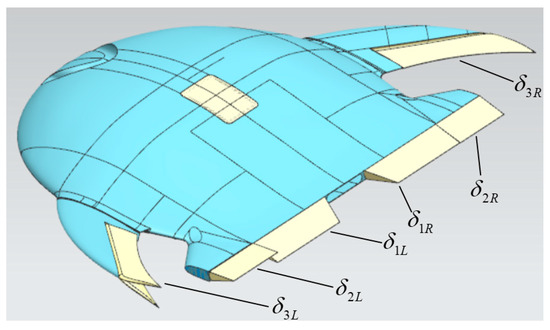
Figure 1. The saucer-shaped unmanned aerial vehicle (UAV) with multiple control surfaces.

The notations of related variables of the UAV are shown in Table 1. This paper mainly focuses on the altitude motion, which can be described by the nonlinear system as follows, similar to the model in Ref. [32].

$$\{\begin{array}{l}\dot{\alpha }=-p\cos \alpha \tan \beta +q-r\sin \alpha \tan \beta -\frac{P\sin \alpha +L-mg\cos \mu \cos \gamma }{mV\cos \beta },\\ \dot{q}=\frac{I_z-I_x}{I_y}pr-\frac{I_{xz}}{I_y}(p^2-r^2)+\frac{M+P{l}_P}{I_y},\\ \dot{\mu }=\frac{P(\sin \alpha \cos \gamma +\cos \alpha \sin \beta \sin \gamma )+L\cos \gamma -Y\sin \gamma -mg\cos \mu }{mV},\\ \dot{h}=V\sin \mu ,\end{array}$$

(1)

Table 1. Main notations and definitions.

Symbol	Variable	Symbol	Variable
$m$$(kg)$	Mass	$V$$(m/s)$	Velocity
$\mu ,\gamma$$(rad)$	Flight path angle andbank angle	$\begin{array}{l}{I}_x,I_y,I_z,I_{xz}\\ (kg\cdot m^2)\end{array}$	Three principal moments of inertia and the product of inertia about the x and z axes
$\alpha ,\beta$$(rad)$	Angle of attack and sideslip	$Q$$(N/m^2)$	Dynamic pressure
$\theta$$(rad)$	Pitch angle	${\rho }_h$$(kg/m^3)$	Atmospheric density
$p,q,r$$(rad/s)$	Roll, pitch and yaw angular rate	$C_{L0},C_{L\alpha }$	Aerodynamic lift coefficients
$L,Y,P$$(N)$	Lift force, side force and thrust	$\begin{array}{l}{C}_{m0},C_{m\alpha },\\ C_{mq},C_{m\delta e}\end{array}$	Aerodynamic pitch coefficients
$M$$(N\cdot m)$	Pitch moment	$S$$(m^2)$	Reference area
$l_P$$(m)$	Position of the engine in the body axis	$c_A$$(m)$	Chord
$g$$(m/s^2)$	Gravitational acceleration	$h$	Altitude

In the longitudinal equation above, the variables for lateral states $p$, $r$, $\beta$ and $\gamma$ are always very small and thus can be simplified to zero and the expression of flight path angle $\mu =\theta -\alpha$ approximately holds.

Considering the configuration illustrated in Figure 1, when the two inboard tailerons are used as an elevator, since the flow condition changes between the adjacent outboard and inboard tailerons surface, inevitably, interactions within control effectors will be introduced. Moreover, as the tailerons are located just behind SDRs, the downstream flow over these effectors will be disturbed by the SDRs; meanwhile, the deflection of SSDs at different attack angles will additively yield lift effects and cross-axis coupled moments. Based on the analysis above, the expression of aerodynamic-related forces and moments $L$ and $M$ are expanded as $L=QS(C_{L0}+C_{L\alpha }\alpha +\Delta C_{L\delta }({\delta }_{1LR},\left|{\delta }_{2LR}\right|,\left|{\delta }_3\right|))$ and $M=QS{c}_A(C_{m0}+C_{m\alpha }\alpha +(C_{mq}\cdot c_A/2V)q+C_{m\delta e}{\delta }_{1LR}+\Delta C_{m\delta }(\left|{\delta }_{2LR}\right|,\left|{\delta }_3\right|))$, where $Q=1/2{\rho }_h{V}^2$ is the dynamic pressure and $C_{L0}$, $C_{L\alpha }$, $C_{m0}$, $C_{m\alpha }$, $C_{mq}$ and $C_{m\delta e}$ denote the aerodynamic derivatives which can be obtained via computational fluid dynamics technique. $\Delta C_{L\delta }(\cdot )$ and $\Delta C_{m\delta }(\cdot )$ denote the uncertain terms caused by the coupling of control surface effects and nonlinear factors.

Without loss of generality [33], velocity $V$ is assumed to be a known constant since the focus of this paper is altitude control and flight path angle $\mu$ is small, i.e., $\sin \mu \approx \mu$. Furthermore, the related dynamics of the altitude in Equation (1) can be rewritten as

$$\{\begin{array}{l}\dot{h}=V\mu ,\\ \dot{\mu }=f_{\mu }+{\phi }_2\theta +d_{\mu },\\ \dot{\theta }=q,\\ \dot{q}=f_{\theta ,\mu ,q}+{\phi }_4{\delta }_{1LR}+d_q,\end{array}$$

(2)

where $f_{\mu }=\frac{QS(C_{L0}-C_{L\alpha }\mu )-mg\cos \mu }{mV}$, ${\phi }_2=\frac{QS{C}_{L\alpha }}{mV}$ and ${\phi }_4=\frac{QS{c}_A{C}_{m\delta e}}{I_y}$ can be seen as constant values here and $f_{\theta ,\mu ,q}=\frac{QS{c}_A}{I_y}(C_{m0}+C_{m\alpha }(\theta -\mu )+C_{mq}\frac{c_A}{2V}q)$, $d_{\mu }=\frac{P\sin \alpha }{mV}+\frac{QS\Delta C_{L\delta }(\cdot )}{mV}+\Delta d_{\mu }$, $d_q=\frac{P{l}_P}{I_y}+\frac{QS{c}_A}{I_y}\Delta C_{m\delta }(\cdot )+\Delta d_q$, $\Delta d_{\mu }$ and $\Delta d_q$ stand for parametric uncertainties and external disturbances, etc.

For the nonlinear system (2), the main control task is to steer the UAV to stably track a desired altitude with a sufficient small tracking error, under the existence of couple effect of multiple control effectors, internal parametric uncertainties and external disturbances. Additionally, $d_{\mu }$ in system (2) is the so-called mismatched disturbance/uncertainty that should be dealt with. To guarantee that the control task is achievable, the following assumption is invoked.

Assumption 1:

The compound disturbances $d_{\mu }$ and $d_q$ and the corresponding derivatives are bounded, namely there exist positive constants $M_{\mu }$, $N_{\mu }$, $M_q$ and $N_q$ satisfying that $\left|d_{\mu }\right|\le M_{\mu }$, $\left|{\dot{d}}_{\mu }\right|\le N_{\mu }$, $\left|d_q\right|\le M_q$ and $\left|{\dot{d}}_q\right|\le N_q$. The first and second time derivatives of the desired altitude reference $h_d$ exist and are bounded.

Remark 1:

The assumption above about disturbance is fairly reasonable, which also has been widely applied all along in the existing literature on ESO-based control and disturbance rejection control [29,30,34]. Specifically, the un-modelled coupled nonlinearity and unknown uncertainties are affected by the flight environment and aircraft effectors structure parameters, which can only change continuously and smoothly. Therefore, the internal uncertainty and its derivatives are bounded. On the other hand, the main causes of external perturbation include complex temperature and pressure changes, wind gusts disturbances, etc. As for a practical physical system, external interference and its time derivatives are obviously limited.

3. Control System Design

In this section, the backstepping technique is employed as an effective systematic tool for controller design to handle the nonlinear characteristics of the saucer-shaped UAV dynamics. The main control development can be accomplished in the following three subsections. Firstly, a finite-time convergent differentiator (FTCD) is introduced to obtain the differential estimations of the previous step virtual control signals, which helps avoid the problem of “explosion of terms”. Secondly, we proposed a nonlinear ESO to generate the estimations of compound disturbance in each control loop. The final subsection presents a detailed backstepping strategy combining the differentiator and ESO from the first two subsections, for which the structure diagram is shown in Figure 2.

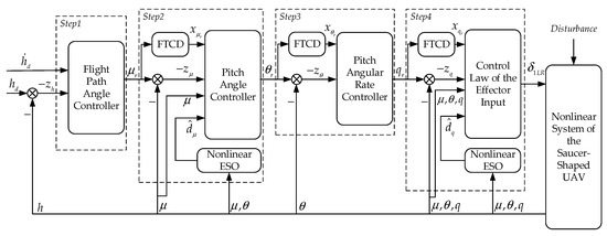
Figure 2. Structure diagram of the proposed control scheme (detailed definition of the symbols in the figure can be found in Section 3.3).

3.1. Finite-Time-Convergent Second-Order Differentiator

So far, many differentiators have been presented to obtain the differential estimation of the system signals in recent decades, such as relatively simple linear differentiator [35], high-order sliding mode based differentiator [36] and sigmoid function-based nonlinear tracking differentiator [37], to name a few. There exists time-lagging phenomenon and chattering problems in the high-order sliding mode-based differentiator, while the nonlinear differentiator has a complicated structure which is hard for parameters to regulate. To address the drawbacks mentioned above, a finite-time convergent differentiator [38] is introduced to the control strategy.

Lemma 1:

[38] The finite-time-convergent second-order differentiator is designed as

$$\{\begin{array}{l}{\dot{x}}_1=x_2,\\ {\epsilon }^2{\dot{x}}_2=-{\mathrm{sat}}_{{\epsilon }_b}\left\{\mathrm{sign}(\varphi (x))\cdot {\left|\varphi (x)\right|}^{\frac{\beta }{2-\beta }}\right\}-{\mathrm{sat}}_{{\epsilon }_b}\left\{\mathrm{sign}(x_2)\cdot {\left|\epsilon x_2\right|}^{\beta }\right\},\\ x_{out}=x_2,\end{array}$$

(3)

where $x_1$, $x_2$ and $x_{out}$ denote the system state and the output of the differentiator, respectively; ${\epsilon }_b>0$ and $\beta \in (0,1)$ are constant; $\epsilon >0$ is a perturbation parameter; $r(t)$ is the input signal of the differentiator; and functions $\varphi (x)$ and ${\mathrm{sat}}_{{\epsilon }_b}(x)$ are defined as follows:

$$\begin{array}{l}\varphi (x)=x_1-r(t)+\frac{\mathrm{sign}(x_2)\cdot {\left|\epsilon x_2\right|}^{2-\beta }}{2-\beta },\\ {\mathrm{sat}}_{{\epsilon }_b}(x)=\{\begin{array}{l}x, \left|x\right|<{\epsilon }_b\\ {\epsilon }_b\mathrm{sign}(x), \left|x\right|\ge {\epsilon }_b\end{array}.\end{array}$$

(4)

For a continuous and piecewise two-order derivable input signal $r(t)$, there exists $\gamma >0$ (where $\rho \gamma >2$ and $\rho =\beta /\left(2-\beta \right)$) and a function $\mathsf{\Gamma }>0$, such that

$$e_i=x_i-r^{(i-1)}(t)=O\left({\epsilon }^{\rho \gamma -i+1}\right).$$

(5)

For $t>\epsilon \mathsf{\Gamma }\left(\Xi (\epsilon )\cdot e(0)\right)$, $i=1$, and $t_j>t\ge t_{j-1}+\epsilon \mathsf{\Gamma }\left(\Xi (\epsilon )\cdot e_{+}(t_{j-1})\right)$, $j=\left\{1,\cdots ,k+1\right\}$, $i=2$, $O({\epsilon }^{\rho \gamma -i+1})$ denotes the approximation of ${\epsilon }^{\rho \gamma -i+1}$ order between $x_i$ and $r^{(i-1)}(t)$, where $\Xi (\epsilon )=\mathrm{diag}\{1,\epsilon \}$, $e\left(0\right)={\left[e_1\left(0\right),e_2\left(0\right)\right]}^T$, $e_{+}\left(t_{j-1}\right)={\left[e_1\left(t_{j-1}\right),e_2^{+}\left(t_{j-1}\right)\right]}^T$, $e_2^{+}\left(t_{j-1}\right)=x_2-{\dot{r}}^{+}\left(t_{j-1}\right)$ and ${\dot{r}}^{+}\left(t_{j-1}\right)$ is the right derivative.

Remark 2:

According to the proof of Wang’s work [38], system (3) is finite-time-convergent. The smaller $\epsilon$ we choose, the shorter the convergent time is and the smaller the tracking errors are. It should be also noted that, if the selected $x_1(0)$ is close to $r(0)$, the peaking phenomenon can be eliminated. Otherwise, we can first select a relatively larger value of $\epsilon$ and then a relatively smaller one after a while.

3.2. Nonlinear ESO Design

Suppose that the nonlinear system dynamic is given by

$$\dot{x}=f(x)+\phi \cdot u+d,$$

(6)

where $x$ is the state, $u$ denotes control input and $d$ represents the total disturbance. $f(x)$ is a known nonlinear function, while $\phi$ used in this paper is a constant expression. Accordingly, Equation (6) has the same form compared with the pitch angular rate and flight path angle loop equations in system (2).

Assumption 2:

The disturbance item $d$ is bounded, and its derivative exists and is also bounded, namely $\max \left\{\left|d\right|,\left|\dot{d}\right|\right\}$ is bounded.

Treat $d$ as the augmented state of the nonlinear system; the nonlinear ESO can be constructed as follows:/

$$\{\begin{array}{l}\dot{\widehat{x}}=f(x)+\phi \cdot u+\widehat{d}+w_1\left[\frac{x-\widehat{x}}{{\varsigma }_1}+w_2\frac{{\varsigma }_1-{\varsigma }_2}{{\varsigma }_2}\cdot \mathrm{sat}\left(\frac{x-\widehat{x}}{{\varsigma }_1{w}_2}\right)\right] , \\ \dot{\widehat{d}}=\frac{w_3}{{\varsigma }_1}\left[\frac{x-\widehat{x}}{{\varsigma }_1}+w_2\frac{{\varsigma }_1^2-{\varsigma }_2^2}{{\varsigma }_2^2}\cdot \mathrm{sat}\left(\frac{x-\widehat{x}}{{\varsigma }_1{w}_2}\right)\right],\end{array}$$

(7)

where $\widehat{x}$ and $\widehat{d}$ are the observer estimated states; $w_i>0$ and ${\varsigma }_j>0$ are positive observer-designing parameters; $i=1,2,3$; and $j=1,2$, satisfying that ${\varsigma }_2<{\varsigma }_1\ll 1$. The symbol $\mathrm{sat}(\cdot )$ represents the standard unity saturation function, which is defined as $\mathrm{sat}(x)=\mathrm{sign}(x)\cdot \min \left\{1,\left|x\right|\right\}$.

Remark 3:

As can be seen from the expressions of $d_{\mu }$ and $d_q$ in Equation (2), the uncertain items (including parametric uncertainties, un-modelled additional force coefficient and coupling torque coefficient) are considered within the composite disturbance. To deal with time-varying disturbances and uncertain or un-modelled dynamics, several potential solutions have been proposed for unmanned vehicles such as the intelligent control method based on recurrent neural networks (NN) [39] and fuzzy logic system (FLS) [40]. The core of these controllers is to adaptively estimate or compensate for the model uncertainties and unknown nonlinear functions approximately based on the universal approximation ability of NN or FLS. He et al. [41] designed two iterative learning control schemes for suppressing the uncertainties and distributed disturbances online. Nevertheless, the above methods suffer from the heavy computational load and slow convergence rate as multiple iterations are needed. During the flight process for the UAV with multiple control surfaces, uncertainties derived from additional force and coupling torque may repeatedly change. To obtain better real-time performance, the proposed observer is adopted to tackle the uncertain dynamics.

Remark 4:

Essentially speaking, in most of the existing literatures, the design process of disturbance observers is a trade-off between the transient performance and the steady-state error. The high-gain observer has advantages in accelerating the convergence speed and in improving the robust performance against large uncertainties, but meanwhile, high gain leads to the notorious peaking value problem in the initial stage caused by different initial values of the system and the ESO. It can be seen in the proposed observer that saturation function is invoked to weaken the peaking value problem. Specifically, in the initial stage, as the estimation error $x-\widehat{x}$ is as large as $\left|x-\widehat{x}\right|/{\varsigma }_1{w}_2>1$, the coefficients of the estimation error are $w_1/{\varsigma }_1$ and $w_3/{\varsigma }_1^2$, and thus, we can achieve relatively fast convergence while avoiding the peaking value problem by selecting an appropriate value of ${\varsigma }_1$ through a simple trial and error procedure. Subsequently, when $\left|x-\widehat{x}\right|/{\varsigma }_1{w}_2\le 1$, the coefficients of the estimation error turn into $w_1/{\varsigma }_2$ and $w_3/{\varsigma }_2^2$, a relatively smaller ${\varsigma }_2$ can lead to a higher gain to reduce the steady-state estimation error. In addition, the performance and stability analysis of the estimation of the disturbance signals $d_{\mu }$ and $d_q$ will be further elaborated in Section 4.

3.3. Backstepping Control Law Design

In this subsection, the backstepping controller design of system (2) is presented step by step by combining with the aforementioned finite-time convergent second-order differentiator and nonlinear ESO.

Step 1: Let $z_h=h-h_d$ and $z_{\mu }=\mu -{\mu }_r$, where ${\mu }_r$ is the virtual control law to be designed later. Considering the Lyapunov function $L_{V1}=\frac{1}{2}{z}_h^2$ and taking the derivative of $L_{V1}$ yields

$${\dot{L}}_{V1}=z_h\cdot {\dot{z}}_h=z_h\left(V{z}_{\mu }+V{\mu }_r-{\dot{h}}_d\right).$$

(8)

Design the virtual control law ${\mu }_r$ (flight path angle controller) as

$${\mu }_r=-\left(\frac{k_1}{V}+\frac{1}{2}\right)z_h+\frac{{\dot{h}}_d}{V},$$

(9)

where $k_1>0$ is a positive constant to be selected.

$${\dot{L}}_{V1}=V{z}_h{z}_{\mu }-\left(k_1+\frac{V}{2}\right)z_h^2\le -k_1{z}_h^2+\frac{V}{2}{z}_{\mu }^2,$$

(10)

Step 2: Let $z_{\theta }=\theta -{\theta }_r$, and construct the Lyapunov function as $L_{V2}=L_{V1}+\frac{1}{2}{z}_{\mu }^2$. From system (2) and Equation (10), one has

$${\dot{L}}_{V2}={\dot{L}}_{V1}+z_{\mu }^{}\left(f_{\mu }+{\phi }_2\theta +d_{\mu }-{\dot{\mu }}_r\right)={\dot{L}}_{V1}+{\phi }_2{z}_{\mu }^{}{z}_{\theta }+z_{\mu }^{}\left(f_{\mu }+{\phi }_2{\theta }_r+d_{\mu }-{\dot{\mu }}_r\right).$$

(11)

Then, we obtain ${\dot{\mu }}_r$ through the differentiator (3) with the input ${\mu }_r$, i.e., $x_{out}=x_2=x_{{\mu }_r}$. From Lemma 1, it can be obtained that ${\dot{\mu }}_r=x_{{\mu }_r}-O\left({\epsilon }_{{\mu }_r}^{\rho \gamma -1}\right)$, and substituting it into Equation (11), one gets

$${\dot{L}}_{V2}={\dot{L}}_{V1}+{\phi }_2{z}_{\mu }{z}_{\theta }+z_{\mu }O\left({\epsilon }_{{\mu }_r}^{\rho \gamma -1}\right)+z_{\mu }\left(f_{\mu }+{\phi }_2{\theta }_r+d_{\mu }-x_{{\mu }_r}\right).$$

(12)

Based on Young’s inequality, the following expressions hold:

$${\phi }_2{z}_{\mu }^{}{z}_{\theta }\le \frac{{\phi }_2^2{z}_{\mu }^2}{4{\lambda }_1^2}+{\lambda }_1^2{z}_{\theta }^2,$$

(13)

$$z_{\mu }^{}O\left({\epsilon }_{{\mu }_r}^{\rho \gamma -1}\right)\le \frac{1}{2}{z}_{\mu }^2+O\left({\epsilon }_{{\mu }_r}^{2\rho \gamma -2}\right),$$

(14)

where ${\lambda }_1>0$ is the design parameter.

Let ${\widehat{d}}_{\mu }$ denote the estimation of $d_{\mu }$, which is generated by the following observer:

$$\{\begin{array}{l}\dot{\widehat{\mu }}=f_{\mu }+{\phi }_2\theta +{\widehat{d}}_{\mu }+w_{1\mu }\left[\frac{\mu -\widehat{\mu }}{{\varsigma }_{1\mu }}+w_{2\mu }\frac{{\varsigma }_{1\mu }-{\varsigma }_{2\mu }}{{\varsigma }_{2\mu }}\cdot \mathrm{sat}\left(\frac{\mu -\widehat{\mu }}{{\varsigma }_{1\mu }{w}_{2\mu }}\right)\right],\\ {\dot{\widehat{d}}}_{\mu }=\frac{w_{3\mu }}{{\varsigma }_{1\mu }}\left[\frac{\mu -\widehat{\mu }}{{\varsigma }_{1\mu }}+w_{2\mu }\frac{{\varsigma }_{1\mu }^2-{\varsigma }_{2\mu }^2}{{\varsigma }_{2\mu }^2}\cdot \mathrm{sat}\left(\frac{\mu -\widehat{\mu }}{{\varsigma }_{1\mu }{w}_{2\mu }}\right)\right],\end{array}$$

(15)

where $w_{1\mu }$, $w_{2\mu }$, $w_{3\mu }$, ${\varsigma }_{1\mu }$ and ${\varsigma }_{2\mu }$ are positive observer parameters to be designed and ${\varsigma }_{2\mu }<{\varsigma }_{1\mu }\ll 1$.

The virtual control law ${\theta }_r$ (pitch angle controller) can be designed as

$${\theta }_r=-\frac{1}{{\phi }_2}\left(z_{\mu }\left(k_2+\frac{V}{2}+\frac{1}{2}+\frac{{\phi }_2^2}{4{\lambda }_1^2}\right)+f_{\mu }+{\widehat{d}}_{\mu }-x_{{\mu }_r}\right),$$

(16)

where $k_2>0$ is a positive parameter to be designed. Substituting Equations (13), (14) and (16) into Equation (12) yields the following:

$${\dot{L}}_{V2}\le -k_1{z}_h^2-k_2{z}_{\mu }^2+{\lambda }_1^2{z}_{\theta }^2+z_{\mu }^{}\left(d_{\mu }-{\widehat{d}}_{\mu }\right)+O\left({\epsilon }_{{\mu }_r}^{2\rho \gamma -2}\right).$$

(17)

Step 3: Define $z_q=q-q_r$, and consider the Lyapunov function $L_{V3}=L_{V2}+\frac{1}{2}{z}_{\theta }^2$. Taking the derivative of $L_{V3}$ yields

$${\dot{L}}_{V3}={\dot{L}}_{V2}+z_{\theta }\left(\dot{\theta }-{\dot{\theta }}_r\right)={\dot{L}}_{V2}+z_{\theta }\left(z_q+q_r-{\dot{\theta }}_r\right).$$

(18)

Let ${\theta }_r$ pass through a second-order differentiator to obtain the estimation for the differentiation of the virtual control law in finite time. Define the differentiator output $x_{out}=x_{{\theta }_r}$; using Lemma 1, we have

$${\dot{\theta }}_r=x_{{\theta }_r}-O\left({\epsilon }_{{\theta }_r}^{\rho \gamma -1}\right).$$

(19)

According to mean-square inequality

$$z_{\theta }O\left({\epsilon }_{{\theta }_r}^{\rho \gamma -1}\right)\le \frac{1}{2}{z}_{\theta }^2+O\left({\epsilon }_{{\theta }_r}^{2\rho \gamma -2}\right),$$

(20)

$$z_{\theta }{z}_q\le \frac{1}{2}{z}_{\theta }^2+\frac{1}{2}{z}_q^2.$$

(21)

From Equations (17)–(21), we obtain that

$${\dot{L}}_{V3}\le -k_1{z}_h^2-k_2{z}_{\mu }^2+{\lambda }_1^2{z}_{\theta }^2+z_{\mu }^{}\left(d_{\mu }-{\widehat{d}}_{\mu }\right)+z_{\theta }^2+\frac{1}{2}{z}_q^2+z_{\theta }\left(q_r-x_{{\theta }_r}\right)+O\left({\epsilon }_{{\mu }_r}^{2\rho \gamma -2}\right)+O\left({\epsilon }_{{\theta }_r}^{2\rho \gamma -2}\right).$$

(22)

Design the virtual control law $q_r$ (pitch angular rate controller) as

$$q_r=-z_{\theta }(k_3+{\lambda }_1^2+1)+x_{{\theta }_r},$$

(23)

where $k_3>0$ is a positive design parameter. Then, together with Equation (22) and Equation (23), one has

$${\dot{L}}_{V3}\le -k_1{z}_h^2-k_2{z}_{\mu }^2-k_3{z}_{\theta }^2+\frac{1}{2}{z}_q^2+z_{\mu }^{}\left(d_{\mu }-{\widehat{d}}_{\mu }\right)+O\left({\epsilon }_{{\mu }_r}^{2\rho \gamma -2}\right)+O\left({\epsilon }_{{\theta }_r}^{2\rho \gamma -2}\right).$$

(24)

Step 4: Choose the Lyapunov function as $L_{V4}=L_{V3}+\frac{1}{2}{z}_q^2$, and compute the derivative of $L_{V4}$ as

$${\dot{L}}_{V4}={\dot{L}}_{V3}+z_q^{}\left(\dot{q}-{\dot{q}}_r\right)={\dot{L}}_{V3}+z_q^{}\left(f_{\theta ,\mu ,q}+{\phi }_4{\delta }_{1LR}+d_q-{\dot{q}}_r\right).$$

(25)

Let $q_r$ pass through a second-order differentiator, and define the differentiator output $x_{q_r}$. By using Lemma 1, it follows that

$${\dot{q}}_r=x_{q_r}-O\left({\epsilon }_{q_r}^{\rho \gamma -1}\right).$$

(26)

The total disturbance $d_q$ in the pitch angular rate loop can be estimated by the following nonlinear ESO

$$\{\begin{array}{l}\dot{\widehat{q}}=f_{\theta ,\mu ,q}+{\phi }_4{\delta }_{1LR}+{\widehat{d}}_q+w_{1q}\left[\frac{q-\widehat{q}}{{\varsigma }_{1q}}+w_{2q}\frac{{\varsigma }_{1q}-{\varsigma }_{2q}}{{\varsigma }_{2q}}\cdot \mathrm{sat}\left(\frac{q-\widehat{q}}{{\varsigma }_{1q}{w}_{2q}}\right)\right],\\ {\dot{\widehat{d}}}_q=\frac{w_{3q}}{{\varsigma }_{1q}}\left[\frac{q-\widehat{q}}{{\varsigma }_{1q}}+w_{2q}\frac{{\varsigma }_{1q}^2-{\varsigma }_{2q}^2}{{\varsigma }_{2q}^2}\cdot \mathrm{sat}\left(\frac{q-\widehat{q}}{{\varsigma }_{1q}{w}_{2q}}\right)\right].\end{array}$$

(27)

where $w_{1q}$, $w_{2q}$, $w_{3q}$, ${\varsigma }_{1q}$ and ${\varsigma }_{2q}$ are positive design parameters and ${\varsigma }_{2\mu }<{\varsigma }_{1\mu }\ll 1$.

From Equations (24)–(26), one can get

$$\begin{array}{ll}{\dot{L}}_{V4}& ={\dot{L}}_{V3}+z_q^{}\left(f_{\theta ,\mu ,q}+{\phi }_4{\delta }_{1LR}+d_q-x_{q_r}+O\left({\epsilon }_{q_r}^{\rho \gamma -1}\right)\right)\\ & \le -k_1{z}_h^2-k_2{z}_{\mu }^2-k_3{z}_{\theta }^2+z_q^2+z_q^{}\left(f_{\theta ,\mu ,q}+{\phi }_4{\delta }_{1LR}+d_q-x_{q_r}\right)\\ & +z_{\mu }^{}\left(d_{\mu }-{\widehat{d}}_{\mu }\right)+O\left({\epsilon }_{{\mu }_r}^{2\rho \gamma -2}\right)+O\left({\epsilon }_{{\theta }_r}^{2\rho \gamma -2}\right)+O\left({\epsilon }_{q_r}^{2\rho \gamma -2}\right).\end{array}$$

(28)

Finally, the controller input can be designed as

$${\delta }_{1LR}=-\frac{1}{{\phi }_4}\left(z_q^{}\left(k_4+1\right)+f_{\theta ,\mu ,q}+{\widehat{d}}_q-x_{q_r}\right),$$

(29)

where $k_4>0$ is a positive constant to be selected. It follows that

$$\begin{array}{ll}{\dot{L}}_{V4}& ={\dot{L}}_{V3}+z_q^{}\left(f_{\theta ,\mu ,q}+{\phi }_4{\delta }_{1LR}+d_q-x_{q_r}+O\left({\epsilon }_{q_r}^{\rho \gamma -1}\right)\right)\\ & \le -k_1{z}_h^2-k_2{z}_{\mu }^2-k_3{z}_{\theta }^2-k_4{z}_q^2+z_q^{}\left(d_q-{\widehat{d}}_q\right)+z_{\mu }^{}\left(d_{\mu }-{\widehat{d}}_{\mu }\right)+O\left({\epsilon }_{{\mu }_r}^{2\rho \gamma -2}\right)+O\left({\epsilon }_{{\theta }_r}^{2\rho \gamma -2}\right)+O\left({\epsilon }_{q_r}^{2\rho \gamma -2}\right).\end{array}$$

(30)

4. Stability and Altitude Tracking Performance Analysis

In this section, the stability of the closed-loop system and the tracking performance will be discussed. The main result is given by the following theorem.

Theorem 1:

Consider the saucer-shaped UAV altitude tracking closed-loop system formed of nonlinear model (1); the ESOs (15) and (27); the second-order differentiators of virtual control signal ${\mu }_r$, ${\theta }_r$ and $q_r$; and the control law (29) with (9), (16) and (23). Assume that Assumption 1 is satisfied; then the proposed control scheme can guarantee the following:

(1) 

All the signals of the resulting closed-loop system remain bounded.

(2) 

The system output tracking error converges to a sufficiently small neighbourhood of zero by selecting appropriate design parameters.

Proof: 

In the first half of the proving process, we mainly focus on the convergences of ESOs. Redefine the scaled ESO estimation error vectors for ESOs (15) and (27) as ${\xi }_x={\left[{\xi }_{1x},{\xi }_{dx}\right]}^T$, in which ${\xi }_{1x}=\left(x-\widehat{x}\right)/{\varsigma }_{1x}$, ${\xi }_{dx}=d_x-{\widehat{d}}_x$ and $x=\mu ,q$. The time derivative of ${\xi }_x$ can be computed as

$$\{\begin{array}{l}{\dot{\xi }}_{1x}=\frac{{\xi }_{dx}}{{\varsigma }_{1x}}-\frac{w_{1x}{\xi }_{1x}}{{\varsigma }_{1x}}-w_{1x}{w}_{2x}\left(\frac{1}{{\varsigma }_{2x}}-\frac{1}{{\varsigma }_{1x}}\right)\mathrm{sat}\left(\frac{{\xi }_{1x}}{w_{2x}}\right),\\ {\dot{\xi }}_{dx}=-\frac{w_{3x}}{{\varsigma }_{1x}}{\xi }_{1x}-\frac{w_{3x}{w}_{2x}}{{\varsigma }_{1x}}\left(\frac{{\varsigma }_{1x}^2}{{\varsigma }_{2x}^2}-1\right)\mathrm{sat}\left(\frac{{\xi }_{1x}}{w_{2x}}\right)+{\dot{d}}_x\end{array} x=\mu ,q.$$

(31)

Consider the Lyapunov function as

$$L_{V{\xi }_x}=\frac{1}{2}{l}_{1x}{\xi }_{1x}^2+\frac{1}{2}{l}_{2x}{\xi }_{dx}^2-l_{3x}{\xi }_{1x}^{}{\xi }_{dx}^{}+l_{4x}{\displaystyle {\int }_0^{{\xi }_{1x}^{}}\mathrm{sat}\left(\frac{{\xi }_{1x}}{w_{2x}}\right)}d{\xi }_{1x}, x=\mu ,q,$$

(32)

where $l_{1x},l_{2x},l_{3x},l_{4x}$ are positive constants and taking the time derivative of $L_{V{\xi }_x}$ along with the formula of (31), one has

$$\begin{array}{ll}{\dot{L}}_{V{\xi }_x}& =\left(l_{1x}{\xi }_{1x}^{}-l_{3x}{\xi }_{dx}^{}+l_{4x}\mathrm{sat}\left(\frac{{\xi }_{1x}}{w_{2x}}\right)\right)\left(\frac{{\xi }_{dx}}{{\varsigma }_{1x}}-\frac{w_{1x}{\xi }_{1x}}{{\varsigma }_{1x}}-w_{1x}{w}_{2x}\left(\frac{1}{{\varsigma }_{2x}}-\frac{1}{{\varsigma }_{1x}}\right)\mathrm{sat}\left(\frac{{\xi }_{1x}}{w_{2x}}\right)\right)\\ & -\left(l_{2x}{\xi }_{dx}^{}-l_{3x}{\xi }_{1x}^{}\right)\left(\frac{w_{3x}}{{\varsigma }_{1x}}{\xi }_{1x}+\frac{w_{3x}{w}_{2x}}{{\varsigma }_{1x}}\left(\frac{{\varsigma }_{1x}^2}{{\varsigma }_{2x}^2}-1\right)\mathrm{sat}\left(\frac{{\xi }_{1x}}{w_{2x}}\right)\right)+\left(l_{2x}{\xi }_{dx}^{}-l_{3x}{\xi }_{1x}^{}\right){\dot{d}}_x\\ & =-\left(\frac{l_{1x}{w}_{1x}-l_{3x}{w}_{3x}}{{\varsigma }_{1x}}\right){\xi }_{1x}^2-\frac{l_{3x}}{{\varsigma }_{1x}}{\xi }_{dx}^2+\left(\frac{l_{1x}+l_{3x}{w}_{1x}-l_{2x}{w}_{3x}}{{\varsigma }_{1x}}\right){\xi }_{1x}^{}{\xi }_{dx}^{}\\ & -\left(\frac{l_{2x}{w}_{3x}{w}_{2x}}{{\varsigma }_{1x}}\left(\frac{{\varsigma }_{1x}^2}{{\varsigma }_{2x}^2}-1\right)-\frac{l_{3x}{w}_{1x}{w}_{2x}}{{\varsigma }_{1x}}\left(\frac{{\varsigma }_{1x}}{{\varsigma }_{2x}}-1\right)-\frac{l_{4x}}{{\varsigma }_{1x}}\right)\mathrm{sat}\left(\frac{{\xi }_{1x}}{w_{2x}}\right){\xi }_{dx}^{}\\ & -\left(\frac{l_{4x}{w}_{1x}}{{\varsigma }_{1x}}+\frac{l_{1x}{w}_{1x}{w}_{2x}}{{\varsigma }_{1x}}\left(\frac{{\varsigma }_{1x}}{{\varsigma }_{2x}}-1\right)-\frac{l_{3x}{w}_{3x}{w}_{2x}}{{\varsigma }_{1x}}\left(\frac{{\varsigma }_{1x}^2}{{\varsigma }_{2x}^2}-1\right)\right)\mathrm{sat}\left(\frac{{\xi }_{1x}}{w_{2x}}\right){\xi }_{1x}^{}\\ & -l_{4x}{w}_{1x}{w}_{2x}\left(\frac{1}{{\varsigma }_{2x}}-\frac{1}{{\varsigma }_{1x}}\right){\mathrm{sat}}^2\left(\frac{{\xi }_{1x}}{w_{2x}}\right)+\left(l_{2x}{\xi }_{dx}^{}-l_{3x}{\xi }_{1x}^{}\right){\dot{d}}_x.\end{array}$$

(33)

Consider that, in Equation (32), the integral ${\displaystyle {\int }_0^{{\xi }_{1x}^{}}\mathrm{sat}\left(\frac{{\xi }_{1x}}{w_{2x}}\right)}d{\xi }_{1x}>0$ holds, as $\mathrm{sat}(\cdot )$ is an odd function. By setting $l_{1x}>l_{3x}$ and $l_{2x}>l_{3x}$, the inequality $\frac{1}{2}{l}_{1x}{\xi }_{1x}^2+\frac{1}{2}{l}_{2x}{\xi }_{dx}^2-l_{3x}{\xi }_{1x}^{}{\xi }_{dx}^{}>\frac{1}{2}\left(l_{1x}-l_{3x}\right){\xi }_{1x}^2+\frac{1}{2}\left(l_{2x}-l_{3x}\right){\xi }_{dx}^2>0$ can be ensured. Thus, the Lyapunov function $L_{V{\xi }_x}$ meets the condition for positive definition.

Select the constants $l_{1x},l_{2x},l_{3x},l_{4x}$ (here, ${\varsigma }_{1x}>{\varsigma }_{2x}$) under the following constrains

$$\{\begin{array}{l}{l}_{1x}>l_{3x},l_{2x}>l_{3x},\\ l_{1x}+l_{3x}{w}_{1x}-l_{2x}{w}_{3x}=0,\\ l_{1x}{w}_{1x}>l_{3x}{w}_{3x},\\ l_{4x}=w_{2x}(l_{2x}{w}_{3x}({\varsigma }_{1x}^2/{\varsigma }_{2x}^2-1)-l_{3x}{w}_{1x}({\varsigma }_{1x}^{}/{\varsigma }_{2x}^{}-1)),\\ w_{3x}(l_{2x}{w}_{1x}-l_{3x})({\varsigma }_{1x}/{\varsigma }_{2x}+1)-w_{1x}(l_{3x}{w}_{1x}-l_{1x})>0,\end{array}$$

(34)

Thus, Equation (32) can be simplified as

$$\begin{array}{ll}{\dot{L}}_{V{\xi }_x}& =-\left(\frac{l_{1x}{w}_{1x}-l_{3x}{w}_{3x}}{{\varsigma }_{1x}}\right){\xi }_{1x}^2-\frac{l_{3x}}{{\varsigma }_{1x}}{\xi }_{dx}^2-l_{4x}{w}_{1x}{w}_{2x}\left(\frac{1}{{\varsigma }_{2x}}-\frac{1}{{\varsigma }_{1x}}\right){\mathrm{sat}}^2\left(\frac{{\xi }_{1x}}{w_{2x}}\right)+\left(l_{2x}{\xi }_{dx}^{}-l_{3x}{\xi }_{1x}^{}\right){\dot{d}}_x\\ & -\left(\frac{w_{3x}{w}_{2x}\left(l_{2x}{w}_{1x}-l_{3x}\right)}{{\varsigma }_{1x}}\left(\frac{{\varsigma }_{1x}^2}{{\varsigma }_{2x}^2}-1\right)-\frac{w_{1x}{w}_{2x}\left(l_{3x}{w}_{1x}-l_{1x}\right)}{{\varsigma }_{1x}}\left(\frac{{\varsigma }_{1x}}{{\varsigma }_{2x}}-1\right)\right)\mathrm{sat}\left(\frac{{\xi }_{1x}}{w_{2x}}\right){\xi }_{1x}^{}. \end{array}$$

(35)

For subsequent use, two compact sets are defined as

$$\begin{array}{l}{S}_1=\left\{{\left[{\xi }_{\mu }^T,{\xi }_q^T\right]}^T\in {ℝ}^4|L_{V\xi }\left({\xi }_{\mu },{\xi }_q\right)=L_{V{\xi }_{\mu }}\left({\xi }_{\mu }\right)+L_{V{\xi }_q}\left({\xi }_q\right)\le D_1\right\},\\ S_2=\left\{{\left[{\xi }_{\mu }^T,{\xi }_q^T\right]}^T\in {ℝ}^4|L_{V\xi }\left({\xi }_{\mu },{\xi }_q\right)\le D_2\right\},\end{array}$$

(36)

where $D_1$ and $D_2$ are positive with $D_2=\underset{\left|{\xi }_{1\mu }\right|\le w_{2\mu },\left|{\xi }_{1q}\right|\le w_{2q}}{\max }\left(L_{V\xi }\left({\xi }_{\mu },{\xi }_q\right)\right)$ and $D_1=\max \left\{D_2,L_{V\xi }\left({\xi }_{\mu }(0),{\xi }_q(0)\right)\right\}$. The proof for convergence of the observers will be split into two steps.

Step 1: Here, we discuss the boundedness of the error vector $\xi ={\left[{\xi }_{\mu }^T,{\xi }_q^T\right]}^T$ for any initial $\xi \in S_1-S_2$; there exists a time instant $t_1$ when $t>t_1$, $\xi \in S_2$ is satisfied. Due to page limitations, a more detailed proof is presented in Appendix A, which is elaborated with four cases.

Step 2: In this step, we prove the convergence of the estimation errors on the basis of the conclusion in Step 1. Since, when $t>t_1$, $\xi ={\left[{\xi }_{\mu }^T,{\xi }_q^T\right]}^T\in S_2$ always holds, which means that $\left|{\xi }_{1\mu }\right|\le w_{2\mu }$ and $\left|{\xi }_{1q}\right|\le w_{2q}$. We introduce a new error vector ${\overline{\xi }}_x={\left[{\xi }_{2x},{\xi }_{dx}\right]}^T$, where ${\xi }_{2x}=\left(x-\widehat{x}\right)/{\varsigma }_{2x}$, $x=\mu ,q$, together with Equation (7), the time derivative of $\overline{\xi }$ is given by

$$\{\begin{array}{l}{\dot{\xi }}_{2x}=\frac{1}{{\varsigma }_{2x}}{\xi }_{dx}-\frac{w_{1x}}{{\varsigma }_{2x}}{\xi }_{2x}\\ {\dot{\xi }}_{dx}={\dot{d}}_x-\frac{w_{3x}}{{\varsigma }_{2x}}{\xi }_{2x}\end{array}, x=\mu ,q,$$

(37)

Consider the Lyapunov function as

$$L_{\mathrm{W}\overline{\xi }}={\displaystyle \sum _{x=\mu ,q}{L}_{\mathrm{W}{\overline{\xi }}_x}}={\displaystyle \sum _{x=\mu ,q}\left(\frac{1}{2}{l}_{1x}{\xi }_{2x}^2+\frac{1}{2}{l}_{2x}{\xi }_{dx}^2-l_{3x}{\xi }_{2x}^{}{\xi }_{dx}^{}\right)},$$

(38)

According to mean-square inequality, it follows that

$$\frac{1}{2}\left(l_{1x}+l_{3x}\right){\xi }_{2x}^2+\frac{1}{2}\left(l_{2x}+l_{3x}\right){\xi }_{dx}^2\ge L_{\mathrm{W}{\overline{\xi }}_x}\ge \frac{1}{2}\left(l_{1x}-l_{3x}\right){\xi }_{2x}^2+\frac{1}{2}\left(l_{2x}-l_{3x}\right){\xi }_{dx}^2,$$

(39)

where the values of $l_{1x},l_{2x},l_{3x},l_{4x}$ are consistent with the analysis in step 1, namely under the constrains of Equation (34). Then, it can be extended from $L_{\mathrm{W}{\overline{\xi }}_x}$ to $L_{\mathrm{W}\overline{\xi }}$ as

$$\frac{1}{2}{\kappa }_{1\mu }\left({\xi }_{2\mu }^2+{\xi }_{d\mu }^2\right)+\frac{1}{2}{\kappa }_{1q}\left({\xi }_{2q}^2+{\xi }_{dq}^2\right)\ge L_{\mathrm{W}\overline{\xi }}\ge \frac{1}{2}{\kappa }_2\left({\xi }_{2\mu }^2+{\xi }_{d\mu }^2+{\xi }_{2q}^2+{\xi }_{dq}^2\right),$$

(40)

where ${\kappa }_{1x}=\max \left(l_{1x}+l_{3x},l_{2x}+l_{3x}\right),{\kappa }_2=\min \left(l_{1\mu }-l_{3\mu },l_{2\mu }-l_{3\mu },l_{1q}-l_{3q},l_{2q}-l_{3q}\right)$.

Depending on Equation (34), computing the time derivative of $L_{\mathrm{W}\overline{\xi }}$ yields

$$\begin{array}{ll}{\dot{L}}_{\mathrm{W}\overline{\xi }}& ={\dot{L}}_{\mathrm{W}{\overline{\xi }}_{\mu }}+{\dot{L}}_{\mathrm{W}{\overline{\xi }}_q}={\displaystyle \sum _{x=\mu ,q}\left(-\frac{l_{1x}{w}_{1x}-l_{3x}{w}_{3x}}{{\varsigma }_{2x}}{\xi }_{2x}^2-\frac{l_{3x}}{{\varsigma }_{2x}}{\xi }_{dx}^2+\left(l_{2x}{\xi }_{dx}^{}-l_{3x}{\xi }_{2x}^{}\right){\dot{d}}_x\right)}\\ & \le {\displaystyle \sum _{x=\mu ,q}\left(-\frac{l_{1x}{w}_{1x}-l_{3x}{w}_{3x}}{{\varsigma }_{2x}}{\xi }_{2x}^2-\frac{l_{3x}}{{\varsigma }_{2x}}{\xi }_{dx}^2+N_x\sqrt{l_{2x}^2+l_{3x}^2}\Vert {\overline{\xi }}_x\Vert \right)},\end{array}$$

(41)

Substituting the Equation (40) into Equation (41), one has

$${\dot{L}}_{\mathrm{W}\overline{\xi }}\le -\frac{{\kappa }_3}{{\varsigma }_2}{L}_{\mathrm{W}\overline{\xi }}+2{\kappa }_4\sqrt{\frac{L_{\mathrm{W}\overline{\xi }}}{{\kappa }_2}},$$

(42)

where ${\kappa }_3=\min \left(\frac{2\left(l_{1\mu }{w}_{1\mu }-l_{3\mu }{w}_{3\mu }\right)}{{\kappa }_{1\mu }},\frac{2l_{3\mu }}{{\kappa }_{1\mu }},\frac{2\left(l_{1q}{w}_{1q}-l_{3q}{w}_{3q}\right)}{{\kappa }_{1q}},\frac{2l_{3q}}{{\kappa }_{1q}}\right)$, ${\kappa }_4=\max \left(N_{\mu }\sqrt{l_{2\mu }^2+l_{3\mu }^2},N_q\sqrt{l_{2q}^2+l_{3q}^2}\right)$ and ${\varsigma }_2=\max \left({\varsigma }_{2\mu },{\varsigma }_{2q}\right)$.

It can be deduced from Equation (42) that, when $L_{\mathrm{W}\overline{\xi }}>\frac{16{\kappa }_4^2{\varsigma }_2^2}{{\kappa }_2{\kappa }_3^2}$, we have ${\dot{L}}_{\mathrm{W}\overline{\xi }}\le -\frac{{\kappa }_3}{2{\varsigma }_2}{L}_{\mathrm{W}\overline{\xi }}<0$. Furthermore, based on the theory of ordinary differential equation, one gets

$$L_{\mathrm{W}\overline{\xi }}\left({\overline{\xi }}_{\mu }\left(t\right),{\overline{\xi }}_q\left(t\right)\right)\le e^{-\frac{{\kappa }_3}{2{\varsigma }_2}\left(t-t_1\right)}{L}_{\mathrm{W}\overline{\xi }}\left({\overline{\xi }}_{\mu }\left(t_1\right),{\overline{\xi }}_q\left(t_1\right)\right).$$

(43)

when $t>t_1$, $\xi \in S_2$ always holds. According to the relationship between ${\overline{\xi }}_x$ and ${\xi }_x$, it can be derived that there exists a constant ${\overline{D}}_2$, such that $L_{\mathrm{W}\overline{\xi }}\left({\overline{\xi }}_{\mu }\left(t_1\right),{\overline{\xi }}_q\left(t_1\right)\right)\le {\overline{D}}_2$. Thus, for $t>t_1+t_2$, where $t_2=\frac{2{\varsigma }_2}{{\kappa }_3}\ln \left(\frac{{\overline{D}}_2}{D_3}\right)$ and $D_3=\frac{16{\kappa }_4^2{\varsigma }_2^2}{{\kappa }_2{\kappa }_3^2}$, we have

$$L_{\mathrm{W}\overline{\xi }}\left({\overline{\xi }}_{\mu }\left(t\right),{\overline{\xi }}_q\left(t\right)\right)\le \frac{16{\kappa }_4^2{\varsigma }_2^2}{{\kappa }_2{\kappa }_3^2}.$$

(44)

Considering Equation (40) with Equation (44), it follows that

$$\Vert {\overline{\xi }}_{\mu }\left(t\right)\Vert +\Vert {\overline{\xi }}_q\left(t\right)\Vert \le \sqrt{2\left({\Vert {\overline{\xi }}_{\mu }\left(t\right)\Vert }^2+{\Vert {\overline{\xi }}_q\left(t\right)\Vert }^2\right)}\le 2\sqrt{\frac{L_{\mathrm{W}\overline{\xi }}\left({\overline{\xi }}_{\mu }\left(t\right),{\overline{\xi }}_q\left(t\right)\right)}{{\kappa }_2}}\le \frac{8{\kappa }_4{\varsigma }_2}{{\kappa }_2{\kappa }_3},$$

(45)

$$\left|d_{\mu }\left(t\right)-{\widehat{d}}_{\mu }\left(t\right)\right|+\left|d_q\left(t\right)-{\widehat{d}}_q\left(t\right)\right|=\left|{\xi }_{d\mu }\left(t\right)\right|+\left|{\xi }_{dq}\left(t\right)\right|<\Vert {\overline{\xi }}_{\mu }\left(t\right)\Vert +\Vert {\overline{\xi }}_q\left(t\right)\Vert \le \frac{8{\kappa }_4}{{\kappa }_2{\kappa }_3}{\varsigma }_2,$$

(46)

$$\left|\mu \left(t\right)-\widehat{\mu }\left(t\right)\right|+\left|q\left(t\right)-\widehat{q}\left(t\right)\right|={\varsigma }_{2\mu }\left|{\xi }_{2\mu }\left(t\right)\right|+{\varsigma }_{2q}\left|{\xi }_{2q}\left(t\right)\right|<{\varsigma }_2\left(\Vert {\overline{\xi }}_{\mu }\left(t\right)\Vert +\Vert {\overline{\xi }}_q\left(t\right)\Vert \right)\le \frac{8{\kappa }_4}{{\kappa }_2{\kappa }_3}{\varsigma }_2^2.$$

(47)

From Equation (46) and Equation (47), it can be concluded that the observer estimation errors converge to a sufficiently small neighbourhood of zero for $t\in (t_1+t_2,+\infty )$, namely

$$\left|d_{\mu }\left(t\right)-{\widehat{d}}_{\mu }\left(t\right)\right|+\left|d_q\left(t\right)-{\widehat{d}}_q\left(t\right)\right|=O\left({\varsigma }_2\right)\mathrm{and}\left|\mu \left(t\right)-\widehat{\mu }\left(t\right)\right|+\left|q\left(t\right)-\widehat{q}\left(t\right)\right|=O\left({\varsigma }_2^2\right).$$

(48)

Let us review the previous definition of the Lyapunov function candidate $L_{V4}$ for the closed-loop system in Section 3, which is specified as $L_{V4}=\frac{1}{2}{z}_h^2+\frac{1}{2}{z}_{\mu }^2+\frac{1}{2}{z}_{\theta }^2+\frac{1}{2}{z}_q^2$. By utilizing mean-square inequality, it can be further deduced from Equation (30) as

$$\begin{array}{ll}{\dot{L}}_{V4}& \le -k_1{z}_h^2-k_2{z}_{\mu }^2-k_3{z}_{\theta }^2-k_4{z}_q^2+z_q^{}\left(d_q-{\widehat{d}}_q\right)+z_{\mu }^{}\left(d_{\mu }-{\widehat{d}}_{\mu }\right)+O({\epsilon }_{{\mu }_r}^{2\rho \gamma -2})+O({\epsilon }_{{\theta }_r}^{2\rho \gamma -2})+O({\epsilon }_{q_r}^{2\rho \gamma -2})\\ & \le -k_1{z}_h^2-\left(k_2-\frac{1}{2}\right)z_{\mu }^2-k_3{z}_{\theta }^2-\left(k_4-\frac{1}{2}\right)z_q^2+\frac{1}{2}{\left(d_q-{\widehat{d}}_q\right)}^2+\frac{1}{2}{\left(d_{\mu }-{\widehat{d}}_{\mu }\right)}^2\\ & +O({\epsilon }_{{\mu }_r}^{2\rho \gamma -2})+O({\epsilon }_{{\theta }_r}^{2\rho \gamma -2})+O({\epsilon }_{q_r}^{2\rho \gamma -2}).\end{array}$$

(49)

From Equation (48), one gets $\frac{1}{2}{\left(d_q-{\widehat{d}}_q\right)}^2+\frac{1}{2}{\left(d_{\mu }-{\widehat{d}}_{\mu }\right)}^2\le \frac{1}{2}{\left(\left|d_q-{\widehat{d}}_q\right|+\left|d_{\mu }-{\widehat{d}}_{\mu }\right|\right)}^2=O\left({\varsigma }_2^2\right)$, and together with Equation (49), we finally achieve that

$$\begin{array}{ll}{\dot{L}}_{V4}& \le -k_1{z}_h^2-\left(k_2-\frac{1}{2}\right)z_{\mu }^2-k_3{z}_{\theta }^2-\left(k_4-\frac{1}{2}\right)z_q^2+O\left({\varsigma }_2^2\right)+O\left({\epsilon }_{{\mu }_r}^{2\rho \gamma -2}\right)+O\left({\epsilon }_{{\theta }_r}^{2\rho \gamma -2}\right)+O\left({\epsilon }_{q_r}^{2\rho \gamma -2}\right)\\ & \le -{\lambda }_V{L}_{V4}+N_V\end{array}$$

(50)

where $k_2$ and $k_4$ are design parameters subject to $k_2>\frac{1}{2}$ and $k_4>\frac{1}{2}$, ${\lambda }_V=\min \left(2k_1,2k_2-1,2k_3,2k_4-1\right)$ and $N_V=O\left({\varsigma }_2^2\right)+O\left({\epsilon }_{{\mu }_r}^{2\rho \gamma -2}\right)+O\left({\epsilon }_{{\theta }_r}^{2\rho \gamma -2}\right)+O\left({\epsilon }_{q_r}^{2\rho \gamma -2}\right)$. Consequently, by solving Equation (50), it yields

$$L_{V4}\left(t\right)\le \frac{N_V}{{\lambda }_V}+\left(L_{V4}\left(0\right)-\frac{N_V}{{\lambda }_V}\right)e^{-{\lambda }_{V}t},$$

(51)

which indicates that all the signals in the closed-loop system are bounded. Moreover, the altitude tracking error can be depicted as

$$\left|z_h\right|\le \sqrt{2\left(\frac{N_V}{{\lambda }_V}+\left(L_{V4}\left(0\right)-\frac{N_V}{{\lambda }_V}\right)e^{-{\lambda }_{V}t}\right)},$$

(52)

Namely $\underset{t\to \infty }{\lim }\left|h-h_d\right|\le \sqrt{\frac{2N_V}{{\lambda }_V}}$. Theoretically, by selecting the arbitrarily small values of ${\varsigma }_{2\mu }$ and ${\varsigma }_{2q}$ in the ESOs and the parameter $\epsilon$ in the differentiator for obtaining a small numerator while choosing relatively large controller law gain $k_i,i=1,\cdots ,4$ in the denominator, it can be concluded that the system output tracking error can converge to a sufficiently small neighbourhood of zero ultimately with less regulation time. This completes the proof of Theorem 1. □

5. Numerical Simulation

In this section, to illustrate the effectiveness of the proposed control scheme, a comparison simulation was carried out. The geometric characteristics, aerodynamic coefficients and other model parameters of the saucer-shaped UAV are given in Table 2. The aerodynamic configuration design philosophy is derived from Ref. [42], especially, since it investigated a sweepback fin-shaped winglet to efficiently reduce the induced drag caused by the low-aspect-ratio configuration. This design is also adopted in the current version of saucer-shaped UAV to improve the aircraft aerodynamic efficiency. In order to give a more intuitive presentation on the aerodynamic characteristics of the saucer-shaped UAV, we made a comparison of the saucer-shaped UAV with a somewhat similar BWB aircraft illustrated in [43]. The typical aerodynamic coefficients of the vehicle in [43] are outlined as $C_{L\alpha }=5.486$, $C_{m\alpha }=-0.1036$ and $C_{mq}=-0.7001$. The saucer-shaped UAV has a smaller lift curve slope $C_{L\alpha }$ as it has larger sweepback and the S-shaped airfoil with a low-aspect-ratio configuration. The pitching moment coefficient $C_{m\alpha }$ of the two aircrafts are negative as both of them have longitudinal static stability, while the aerodynamic centre of the saucer-shaped UAV is located further forward. The absolute value of pitch-damping coefficient of the saucer-shaped UAV, $\left|C_{mq}\right|$, is less than that of the BWB aircraft in [43], which leads to a smaller damping ratio in the short-period mode.

Table 2. Parameters of the saucer-shaped unmanned aerial vehicle.

Parameter	Value	Parameter	Value
Mass $m$(kg)	13	$C_{L0}$	0.0752
Reference area $S$(m2)	2.097	$C_{L\alpha }$	0.03865
Chord $c_A$(m)	0.97991	$C_{m0}$	−0.0181
Air density ${\rho }_h$(kg/m3)	1.225064	$C_{m\alpha }$	−0.0261
Inertial moment $I_y$(kgm2)	1.79715	$C_{mq}$	−0.04
Gravitational acceleration $g$(m/s2)	9.8	$C_{m\delta e}$	−0.18

The main task is to steer the vehicle to track the prescribed altitude reference. To be specific, the initial flight condition was assumed as $h_0=350m$, ${\mu }_0=0deg$, ${\alpha }_0=3.41deg$ and $q_0=0deg/s$, and the command reference starts at the initial altitude and ends at the altitude of $450m$. Besides, the command $h_d$ was smoothened through a filter described as $0.02/\left(s^2+0.3s+0.02\right)$. To confirm the superiority and effectiveness of the proposed ESO, 15% of uncertainties of aerodynamic coefficients were introduced to the actual vehicle model. The disturbances imposed on the flight path angle loop and pitch angular rate loop are taken as $0.5\sin (0.3t)+2.5e^{-0.2t}\sin (1.2t)$ and $2\sin (0.4t)+12e^{-0.09t}\sin (0.8t)$, respectively, which includes the un-modelled coupling effects and external disturbances. Moreover, to further illustrate the robustness of the proposed scheme, an abrupt disturbance of additional constant moment is introduced at the instant $t=60s$, with the value $10N\cdot m$ and duration $\Delta t=0.5s$.

The design parameters for the finite-time-convergent second-order differentiator were chosen as ${\epsilon }_b=1$, $\beta =1/3$ and $\epsilon =0.006$. According to the design principle of the ESO in Section 3.2 and the analysis in Remark 4, the corresponding parameters were set as $w_{1\mu }=4$, $w_{2\mu }=8$, $w_{3\mu }=2$, ${\varsigma }_{1\mu }=0.5$ and ${\varsigma }_{2\mu }=0.05$ for the ESO in the $\mu$ loop and $w_{1q}=1.5$, $w_{2q}=10$, $w_{3q}=0.5$, ${\varsigma }_{1q}=0.1$ and ${\varsigma }_{2q}=0.02$ for the ESO in the $q$ loop. Considering that the backstepping control laws $k_i,i=1,\cdots ,4$ are key factors to determine the convergence rate of the tracking error, we select the control gains as $k_1=5$, $k_2=7$, $k_3=8$ and $k_4=10$ to achieve good tracking performance and transition performance. Besides the proposed control scheme, the adaptive backstepping method derived from Reference [44] is also simulated for comparison purposes (hereafter referred as the compared controller) and the parameters are taken as the same as that of [44]. The compared controller is based on barrier Lyapunov function (BLF) and employs a command filter to obtain the constrained virtual controls and their time derivatives in the back-stepping design process. As the controller is essentially a kind of adaptive backstepping approach depending on nominal values of the aerodynamic coefficients, theoretically, the static uncertainties and disturbances can be handled by adaptive laws.

The simulation results are shown in Figure 3, Figure 4, Figure 5, Figure 6, Figure 7, Figure 8 and Figure 9. Figure 3 depicts the comparative curves with respect to the altitude tracking performance of the two controllers, which can guarantee the boundedness of the altitude tracking error in the presence of internal uncertainties and generalized disturbances. It is obvious that the proposed scheme has better transient and steady-state performance, as the amplitude of the tracking error is less than $0.5m$ in the oscillating process and further falls within the range of $\pm 0.2m$ for $t>20s$; while in the compared scheme, the mechanism of disturbance and uncertainty suppression is based on adaptive control rather than extended state estimation, the performance of the compared controller deteriorates significantly when the time-varying disturbances are taken into account. The noteworthy flight states in the inner loop are illustrated in Figure 4, Figure 5 and Figure 6, which include flight path angle $\mu$, angle of attack $\alpha$ and pitch angular rate $q$ and their time responses are smooth signals in a reasonable range. In particular, with the help of the FTCDs in the proposed controller, flight path angle and angle of attack can reach their steady-state values with more rapid convergence rate and mild fluctuations, even when the abrupt disturbance occurred at $t=60s$. When the altitude command tends to be constant, flight path angle and pith angle rate vary slowly and converge to zero; therefore, the permissible angle of attack is guaranteed. Figure 7 exhibits the comparison curves of control inputs. Under a proposed controller, the max deflection angle is 11.1 deg. The deflection of control effector has a smoother transient process than the response in the compared controller, which can reduce the requirement of actuator bandwidth in practice.

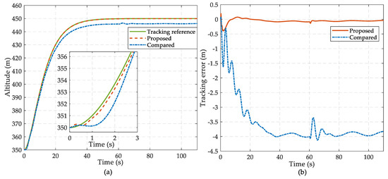
Figure 3. The saucer-shaped UAV altitude tracking performance: (a) Comparison of the response of altitude tracking and (b) comparison of the altitude tracking error.

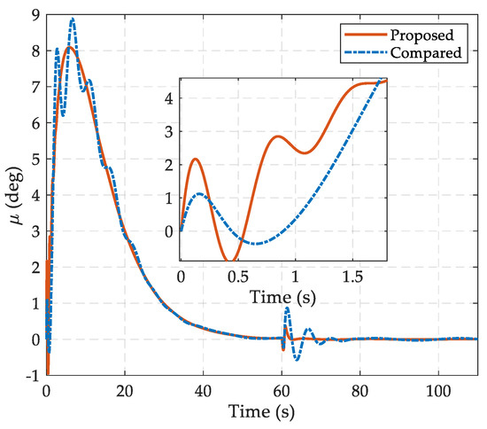
Figure 4. The curves of flight path angle $\mu$ in the comparative simulations.

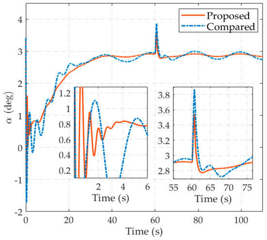
Figure 5. The curves of angle of attack $\alpha$ in the comparative simulations.

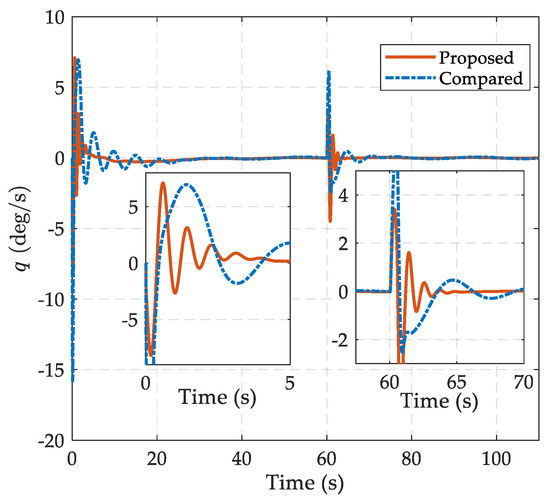
Figure 6. The curves of pitch angular rate $q$ in the comparative simulations.

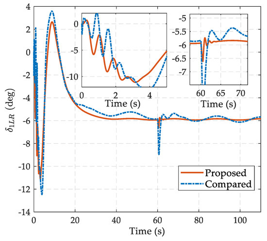
Figure 7. The curves of the deflection of control effector ${\delta }_{1LR}$ in the comparative simulations.

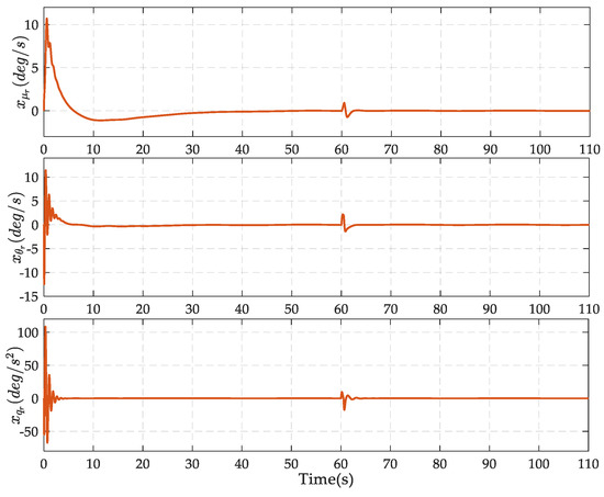
Figure 8. The time derivatives of the intermediate virtual control law $x_{{\mu }_r}$, $x_{{\theta }_r}$ and $x_{q_r}$ obtained by finite-time convergent differentiators (FTCDs).

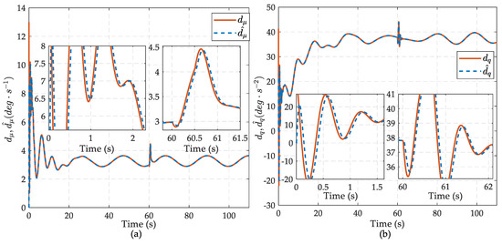
Figure 9. The output of the extended state observers (ESOs): (a) The compound disturbances and its estimation in the flight path angle loop and (b) the compound disturbances and its estimation in the pitch angular rate loop.

Besides, the derivatives of intermediate virtual law obtained by FTCDs are shown in Figure 8. Obviously, the FTCDs provide bounded, continuous and smooth estimations such that the problem of “explosion of complexity” has been eliminated. Meanwhile, the good performance of the proposed method is also attributed to the ability of the ESO in a timely accurate estimation of the compound disturbances composed with modelling uncertainties and external disturbances. As shown in Figure 9, disturbance estimations can track the actual disturbance signals in the first two seconds and have fairly small estimation error margins thereafter.

6. Conclusions

This study has presented a composite backstepping controller towards the disturbance and uncertainty suppression control for a saucer-shaped BWB UAV. To overcome the inherent problem of “explosion of complexity” in the backstepping design, the finite-time convergent differentiator is introduced at each step to avoid tedious analytic computation. Also, a nonlinear extended state observer is proposed to provide online estimation for the compound general disturbance without the peaking value problem. Rigorous proof for the stability of the closed-loop systems and the tracking performance analysis is achieved. In the end, the simulation results indicated and verified the effectiveness and superiority of the proposed method. To extend the proposed method, more constraint conditions can be taken into consideration in future work, such as input saturations and actuator dead-zones. The authors will also pay more attention to validation of the proposed method through outdoor flight experiments with the real UAV.

References

- Richard, W.; Bauer, X. Flying wings/flying fuselages. In Proceedings of the 39th Aerospace Sciences Meeting and Exhibit, Reno, NV, USA, 8–11 January 2011. [Google Scholar]
- De Vries Pieter, S.; van Kampen, E.-J. Reinforcement Learning-based Control Allocation for the Innovative Control Effectors Aircraft. In Proceedings of the AIAA Scitech 2019 Forum, San Diego, CA, USA, 7–11 January 2019. [Google Scholar]
- Okonkwo, P.; Smith, H. Review of evolving trends in blended wing body aircraft design. Prog. Aerosp. Sci. 2016, 82, 1–23. [Google Scholar] [CrossRef]
- Liu, C.J.; Chen, W.H.; Andrews, J. Tracking control of small-scale helicopters using explicit nonlinear MPC augmented with disturbance observers. Control. Eng. Pract. 2012, 20, 258–268. [Google Scholar] [CrossRef]
- Pu, Z.; Tan, X.; Fan, G.; Yi, J. Uncertainty analysis and robust trajectory linearization control of a flexible air-breathing hypersonic vehicle. Acta Astronaut. 2014, 101, 16–32. [Google Scholar] [CrossRef]
- Qiu, B.B.; Wang, G.F.; Fan, Y.S. Trajectory Linearization-Based Adaptive PLOS Path Following Control for Unmanned Surface Vehicle with Unknown Dynamics and Rudder Saturation. Appl. Sci. 2020, 10, 3538. [Google Scholar] [CrossRef]
- Tian, B.L.; Qun, Z.Q. Quasi-continuous high-order sliding mode controller and observer design for vehicle. In Proceedings of the 17th AIAA International Space Planes and Hypersonic Systems and Technologies Conference, San Francisco, CA, USA, 11–14 April 2011. [Google Scholar]
- Denieul, Y.; Bordeneuve-Guibe, J.; Alazard, D.; Toussaint, C.; Taquin, G. Integrated design of flight control surfaces and laws for new aircraft configurations. IFAC-Pap. Online 2017, 50, 14180–14187. [Google Scholar] [CrossRef]
- Wen, N.; Liu, Z.H.; Sun, Y.; Zhu, L.P. Design of LPV-based sliding mode controller with finite time convergence for a morphing aircraft. Int. J. Aerosp. Eng. 2017, 7, 81515–81531. [Google Scholar] [CrossRef]
- Yang, J.; Li, S.H.; Yu, X.H. Sliding-mode control for systems with mismatched uncertainties via a disturbance observer. IEEE Trans. Ind. Electron. 2012, 60, 160–169. [Google Scholar] [CrossRef]
- Chen, W.H.; Yang, J.; Guo, L.; Li, S.H. Disturbance-observer-based control and related methods—An overview. IEEE Trans. Ind. Electron. 2015, 63, 1083–1095. [Google Scholar] [CrossRef]
- Kim, K.S.; Park, Y.J.; Oh, S.H. Designing robust sliding hyperplanes for parametric uncertain systems: A Riccati approach. Automatica 2000, 36, 1041–1048. [Google Scholar] [CrossRef]
- Guo, B.Z.; Wu, Z.H. Active disturbance rejection control approach to output-feedback stabilization of lower triangular nonlinear systems with stochastic uncertainty. Int. J. Robust Nonlin. Control. 2017, 27, 2773–2797. [Google Scholar] [CrossRef]
- Zhao, Z.L.; Guo, B.Z. Active disturbance rejection control approach to stabilization of lower triangular systems with uncertainty. Int. J. Robust Nonlin. Control. 2016, 16, 2314–2337. [Google Scholar] [CrossRef]
- Sun, H.B.; Guo, L. Composite adaptive disturbance observer based control and back-stepping method for nonlinear system with multiple mismatched disturbances. J. Frankl. Inst. 2014, 351, 1027–1041. [Google Scholar] [CrossRef]
- Zhai, D.; An, L.W.; Dong, J.X.; Zhang, Q.L. Robust adaptive fuzzy control of a class of uncertain nonlinear systems with unstable dynamics and mismatched disturbances. IEEE Trans. Cybern. 2017, 48, 3105–3115. [Google Scholar] [CrossRef]
- Shi, X.Y.; Cheng, Y.H.; Yin, C.; Huang, X.G.; Zhong, S.M. Design of adaptive backstepping dynamic surface control method with RBF neural network for uncertain nonlinear system. Neurocomputing 2019, 330, 490–503. [Google Scholar] [CrossRef]
- Yu, J.P.; Ma, Y.M.; Yu, H.S.; Lin, C. Adaptive fuzzy dynamic surface control for induction motors with iron losses in electric vehicle drive systems via backstepping. Inf. Sci. 2017, 376, 172–189. [Google Scholar] [CrossRef]
- Yu, J.P.; Shi, P.; Dong, W.J.; Yu, H.S. Observer and command-filter-based adaptive fuzzy output feedback control of uncertain nonlinear systems. IEEE Trans. Ind. Electron. 2015, 62, 5962–5970. [Google Scholar] [CrossRef]
- Jin, Z.J.; Zhang, W.M.; Liu, S.; Gu, M. Command-Filtered Backstepping Integral Sliding Mode Control with Prescribed Performance for Ship Roll Stabilization. Appl. Sci. 2019, 9, 4288. [Google Scholar] [CrossRef]
- Jiang, T.; Lin, D.F.; Song, T. Finite-time backstepping control for quadrotors with disturbances and input constraints. IEEE Access. 2018, 6, 62037–62049. [Google Scholar] [CrossRef]
- Yu, J.P.; Shi, P.; Zhao, L. Finite-time command filtered backstepping control for a class of nonlinear systems. Automatica 2018, 9, 173–180. [Google Scholar] [CrossRef]
- Zhao, Z.L.; Guo, B.Z. Extended state observer for uncertain lower triangular nonlinear systems. Syst. Control. Lett. 2015, 85, 100–108. [Google Scholar] [CrossRef]
- Gong, L.G.; Wang, Q.; Dong, C.Y. Disturbance rejection control of morphing aircraft based on switched nonlinear systems. Nonlinear Dyn. 2019, 96, 975–995. [Google Scholar] [CrossRef]
- Zhang, L.; Li, Z.; Yang, C. Adaptive neural network based variable stiffness control of uncertain robotic systems using disturbance observer. IEEE Trans. Ind Electron. 2017, 64, 2236–2245. [Google Scholar] [CrossRef]
- Yao, J.; Jiao, Z.; Ma, D. Extended-state-observer-based output feedback nonlinear robust control of hydraulic systems with backstepping. IEEE Trans. Ind. Electron. 2014, 61, 6285–6293. [Google Scholar] [CrossRef]
- Shao, X.L.; Liu, J.; Wang, H.L. Robust back-stepping output feedback trajectory tracking for quadrotors via extended state observer and sigmoid tracking differentiator. Mech. Syst. Signal. Process. 2018, 104, 631–647. [Google Scholar] [CrossRef]
- Xiong, S.; Xie, H.; Song, K.; Zhang, G.H. A Speed Tracking Method for Autonomous Driving via ADRC with Extended State Observer. Appl. Sci. 2019, 9, 3339. [Google Scholar] [CrossRef]
- Li, S.H.; Yang, J.; Chen, W.H.; Chen, X.S. Generalized extended state observer based control for systems with mismatched uncertainties. IEEE Trans. Ind. Electron. 2011, 59, 4792–4802. [Google Scholar] [CrossRef]
- Guo, B.Z.; Zhao, Z.L. On the convergence of an extended state observer for nonlinear systems with uncertainty. Syst. Control. Lett. 2011, 60, 420–430. [Google Scholar] [CrossRef]
- Xing, Z.H.; Wu, S.T.; Wu, X.L. Explicit nonlinear model predictive control for a saucer-shaped unmanned aerial vehicle. Adv. Mech. Eng. 2013, 5, 706453. [Google Scholar] [CrossRef]
- Liu, J.L.; Zhang, W.G.; Liu, X.X.; He, Q.Z.; Qin, Y.X. Gust response stabilization for rigid aircraft with multi-control-effectors based on a novel integrated control scheme. Aerosp. Sci. Technol. 2018, 79, 625–635. [Google Scholar] [CrossRef]
- Wong, K.Y.; Kariya, N.; Tanaka, M.; Tanaka, K. Longitudinal Fuzzy Model Construction of a Flying-Wing Unmanned Aerial Vehicle and a Nonlinear Guaranteed Cost Control Approach to Altitude Stabilization. In Proceedings of the 2019 International Conference on Fuzzy Theory and Its Applications (iFUZZY), New Taipei City, Taiwan, 7–10 November 2019. [Google Scholar]
- Ran, M.P.; Wang, Q.; Dong, C.Y. Active disturbance rejection control for uncertain nonaffine-in-control nonlinear systems. IEEE T. Automat. Contr. 2016, 62, 5830–5836. [Google Scholar] [CrossRef]
- Guo, B.Z.; Han, J.Q.; Xi, F.B. Linear tracking-differentiator and application to online estimation of the frequency of a sinusoidal signal with random noise perturbation. Int. J. Syst. Sci. 2002, 33, 351–358. [Google Scholar] [CrossRef]
- Levant, A. Higher-order sliding modes, differentiation and output-feedback control. Int. J. Control. 2003, 76, 924–941. [Google Scholar] [CrossRef]
- Shao, X.L.; Wang, H.L. Back-stepping robust trajectory linearization control for hypersonic reentry vehicle via novel tracking differentiator. J. Franklin Inst. 2016, 353, 1957–1984. [Google Scholar] [CrossRef]
- Wang, X.H.; Chen, Z.Q.; Yang, G. Finite-time-convergent differentiator based on singular perturbation technique. IEEE Trans. Automat. Contr. 2007, 52, 1731–1737. [Google Scholar] [CrossRef]
- Kuo, C.W.; Tsai, C.C.; Lee, C.T. Intelligent leader-following consensus formation control using recurrent neural networks for small-size unmanned helicopters. IEEE Trans. Syst. Man Cybern. Syst. 2019, 99, 1–14. [Google Scholar] [CrossRef]
- Choi, Y.H.; Sung, J.Y. A simple fuzzy-approximation-based adaptive control of uncertain unmanned helicopters. Int. J. Control. Autom. Syst. 2016, 14, 340–349. [Google Scholar] [CrossRef]
- He, W.; Meng, T.T.; He, X.Y.; Sun, C.Y. Iterative learning control for a flapping wing micro aerial vehicle under distributed disturbances. IEEE Trans. Cybern. 2018, 49, 1524–1535. [Google Scholar] [CrossRef]
- Yu, J.L.; Wang, L.L.; Gao, G. Using wing tip devices to improve performance of saucer-shaped aircraft. Chin. J. Aeronaut. 2006, 19, 309–314. [Google Scholar] [CrossRef]
- Rahman, N.U.; Whidborne, J.F.; Cooke, A.K. Longitudinal control system design and handling qualities assessment of a blended wing body aircraft. In Proceedings of the 6th International Bhurban Conference on Applied Sciences & Technology, Islamabad, Pakistan, 19–22 January 2009; pp. 177–186. [Google Scholar]
- Hao, A.; Xia, H.W.; Wang, C.H. Barrier Lyapunov function-based adaptive control for hypersonic flight vehicles. Nonlinear Dyn. 2017, 88, 1833–1853. [Google Scholar]
© 2020 by the authors. Licensee MDPI, Basel, Switzerland. This article is an open access article distributed under the terms and conditions of the Creative Commons Attribution (CC BY) license (http://creativecommons.org/licenses/by/4.0/).