Forward Transformation from Reactive Near-Field to Near and Far-Field at Millimeter-Wave Frequencies

Abstract

With the advent of 5G mobile communications at millimeter-wave frequencies, the assessment of the maximum averaged power density on numerous surfaces close to the transmitter will become a requirement. This makes phasor knowledge about the electric and magnetic fields an inevitable requirement. To avoid the burdensome measurement of these field quantities in the entire volume of interest, phase reconstruction algorithms from measurements over a plane in the far-field region are being extensively developed. In this paper, we extended the previously developed method of phase reconstruction to evaluate the near and far-field of sources with bounded uncertainty, which is robust with respect to noisy data and optimized for a minimal number of measurement points at a distance as close as $\lambda$/5 from the source. The proposed procedure takes advantage of field integral equations and electric field measurements with the EUmmWVx probe to evaluate the field phasors close to the radiation source and subsequently obtain the field values in the whole region of interest with minimal computation and measurement costs. The main constraints are the maximal noise level regarding the peak electric field and measurement plane size with respect to the percentage of transmitted power content. The measurement of a third plane overcomes some of the noise issues. The method was evaluated by simulations of a wide range of antennas at different noise levels and at different distances and by measurements of four different antennas. A successful reconstruction in the near and far-field was achieved both qualitatively and quantitatively for distances between 2.5–150 mm from the antenna and noise levels of −24 dB from the peak. The deviation of reconstruction from the simulation reference for the peak spatial-average power density with an averaging area of 1 cm${}^2$ was, in all cases, well within the uncertainty budget of 0.6 dB, if the reconstruction planes captured >95% of the total radiated power. The proposed new method is very promising for compliance assessment and can reduce test time considerably.

1. Introduction

Exposure assessment above 10 GHz is typically done by evaluating the power density (PD) at the exposure plane [1,2], which can be obtained through the electric (E-) and magnetic (H-) fields at that plane. Depending on the application, the exposure plane may be very close to the antenna under test (AUT), or further away. To determine the safe operating distance, knowledge about the field in the full volume away from the AUT is required. Such knowledge is also valuable for the research and development of radiating (millimeter-wave) devices.

It is usually time-consuming to measure the full volume of interest; however, rather than measuring the full volume, it is possible to reconstruct the electromagnetic field (EMF) from a set of suitable measurements, as the field is constrained by Maxwell’s equations. For this purpose, the reliable measurement of both the magnitude and phase of the radiated field is required [3,4,5]. However, the development of measurement instruments that capture the varying phase of the quantities becomes more difficult and costly with increasing frequency. As a result, the proper characterization of antennas often relies on phaseless (sometimes referred to as magnitude-only or intensity-only) measurements. Subsequently, the acquired phaseless data are used to reconstruct the phasors through a so-called phase-reconstruction (PR) algorithm.

In the pioneering work of Gerchberg-Saxton [6] and Fienup [7], the PR problem was solved using an alternating projection method, also known as the plane-to-plane (PTP) backpropagation method. The proposed method iteratively estimates the missing phases of the measurements at two sufficiently separate surfaces and performs a field propagation between the two scans. The measurement layer (most often a plane) is usually placed at a distance of a few wavelengths from the AUT. Various modifications of the PTP method were later successfully applied for different antenna problems [8,9,10,11,12,13,14,15,16,17,18]. Some usual limitations of the developed procedures include the requirement of a huge number of measurement points (depending on the beam pattern) and limitations on the propagation geometry, which is required to be the same as the measurement surface. Based on these research efforts [8,9,10,11,12,13,14,15,16,17,18], commercial systems have been developed to perform PR in the far field.

Typical reconstruction algorithms aim at obtaining the E- and H- field phasors in the far-field region. Nevertheless, the reactive near field is becoming increasingly important for consumer millimeter-wave devices. The already proposed methods in the literature are limited in terms of reconstructing the reactive components at distances closer than the measurement plane when using backpropagation.

This paper presents a forward transformation (FT) approach to reconstruct the EMF in the full half-space above a measurement plane that is placed at a distance of 2 mm from the AUT. The approach leverages the well-known field integral equations [19] and the millimeter-wave probe EUmmWVx [20], which allows measurements of the E-field very close to the source—i.e., at distances of a fraction of the wavelength—with minimal probe-related distortions of the field at frequencies up to 110 GHz. This property results in a characterization mechanism that only requires few measurements close to the AUT to capture the whole radiated power, thereby reducing the overall computation and measurement cost for the AUT. To obtain the phase information in the near-field region, we employed the phase reconstruction algorithm developed in [21]. The obtained field phasors are used to evaluate the far-field radiation pattern using the expression of the field profile as an equivalent distribution of dipole moments [22,23,24]. The plane of equivalent currents is placed at the measurement plane very close to the AUT, where the availability of amplitude information of the E-field drastically facilitates the solution of the resulting inverse-source problem. This is in contrast to the source reconstruction methods found in the literature, which typically place measurements much further away than reconstructed equivalent current sources [25,26,27].

The manuscript is structured as follows: After this introduction, Section 2 presents the method used for FT in detail, followed by Section 3 and Section 4, which describe the set of simulation antennas operating at 10, 30, 60 and 90 GHz and the error metric used for algorithm evaluation. The theory behind the approach assumes an infinitely large plane; however, in practice, this plane needs to be truncated at a boundary. The main criteria for the appropriate truncation of this plane are discussed in Section 5. Section 6 describes the evaluation of the algorithm at different noise levels and distances. The results of the simulation study are presented in Section 7. The method is validated with measurements in Section 8.

2. Equivalent Current Reconstruction and FT Approach

The vital piece of hardware in this work that enables phase reconstruction in the near-field domain is the EUmmWVx probe. This probe enables E-field measurements very close to the source with minimal probe-related distortions of the field at frequencies up to 110 GHz. The probe is based on the pseudo-vector probe design [28] which measures not only the magnitude of the field but also derives its polarization ellipse from different probe rotation angles.

Based on these measurements on two planes, a PTP algorithm has been developed that permits the reconstruction of the PD on measurement planes as close as 2 mm distant from the source [21]. This algorithm also yields reconstructed phases of the E and H-fields on the measurement plane, such that equivalent current distributions can be computed using Love’s equivalence theorem [19]. For more details on the probe functionality as well as the reconstruction algorithm, please see [20,28] and [21], respectively.

For closed surfaces (or infinitely large planes), the radiation integrals yield the E and H-fields anywhere outside this surface of equivalent currents. Section 5 investigates the requirements on a proper plane truncation without deteriorating the final outcomes. For planar surfaces, we can further use image theory:

$$\mathbf{M}=2\mathbf{E}\times \mathbf{n},\mathbf{J}=0,$$

(1)

where $\mathbf{M}$ is the magnetic surface current vector, $\mathbf{E}$ is the E-field vector, $\mathbf{n}$ is the unit vector normal to the surface and $\mathbf{J}$ is the electric surface current vector.

The E and H-fields can thus be computed at any point $\mathbf{r}$ in the half-space above the plane of equivalent currents (see [29]):

$$\left[\begin{array}{c}{E}_x\left(\mathbf{r}\right)\\ E_y\left(\mathbf{r}\right)\\ E_z\left(\mathbf{r}\right)\end{array}\right]=\left[\begin{array}{cc}0& -G_z\left(\mathbf{r}\right)\\ G_z\left(\mathbf{r}\right)& 0\\ -G_y\left(\mathbf{r}\right)& G_x\left(\mathbf{r}\right)\end{array}\right]·\left[\begin{array}{c}{\mathbf{M}}_x\\ {\mathbf{M}}_y\end{array}\right].$$

(2)

In this case, ${\mathbf{M}}_x$ and ${\mathbf{M}}_y$ are the equivalent magnetic surface currents tangential to the planar surface, represented as pulse basis functions [30] discretized on a regular grid that coincides with the measurement points, and $G_x\left(\mathbf{r}\right)$, $G_y\left(\mathbf{r}\right)$ and $G_z\left(\mathbf{r}\right)$ are the discretized integrals of the free-space Green’s function at the point $\mathbf{r}=(x,y,z)$, derived with respect to x, y and z [30]. They are matrices of dimensions $1\times n_{\mathrm{src}}$, where $n_{\mathrm{src}}$ is the length of the vectors ${\mathbf{M}}_x$, ${\mathbf{M}}_y$. A simple matrix multiplication then yields the field components $E_x$, $E_y$, $E_z$ at the point $\mathbf{r}$. In other words, the ith element of the matrices $G_x\left(\mathbf{r}\right)$, $G_y\left(\mathbf{r}\right)$, $G_z\left(\mathbf{r}\right)$—respectively, $G_x^i$, $G_y^i$, and $G_z^i$—represent the radiated field of the ith magnetic current element at the observation point $\mathbf{r}$. The value of this element is found from

$$\begin{array}{c}{\displaystyle G_x^i=-\frac{1}{4\pi }\underset{S^i}{\int }\frac{\partial }{\partial x}\frac{e^{-j{k}_0|\mathbf{r}-{\mathbf{r}}_0|}}{|\mathbf{r}-{\mathbf{r}}_0|}\mathrm{d}s=\frac{1}{4\pi }\underset{S^i}{\int }\frac{e^{-j{k}_0|\mathbf{r}-{\mathbf{r}}_0|}}{|\mathbf{r}-{\mathbf{r}}_0{|}^2}(x-x_0)\left(j{k}_0+\frac{1}{|\mathbf{r}-{\mathbf{r}}_0|}\right)\mathrm{d}s}\hfill \\ {\displaystyle G_y^i=-\frac{1}{4\pi }\underset{S^i}{\int }\frac{\partial }{\partial y}\frac{e^{-j{k}_0|\mathbf{r}-{\mathbf{r}}_0|}}{|\mathbf{r}-{\mathbf{r}}_0|}\mathrm{d}s=\frac{1}{4\pi }\underset{S^i}{\int }\frac{e^{-j{k}_0|\mathbf{r}-{\mathbf{r}}_0|}}{|\mathbf{r}-{\mathbf{r}}_0{|}^2}(y-y_0)\left(j{k}_0+\frac{1}{|\mathbf{r}-{\mathbf{r}}_0|}\right)\mathrm{d}s}\hfill \\ {\displaystyle G_z^i=-\frac{1}{4\pi }\underset{S^i}{\int }\frac{\partial }{\partial z}\frac{e^{-j{k}_0|\mathbf{r}-{\mathbf{r}}_0|}}{|\mathbf{r}-{\mathbf{r}}_0|}\mathrm{d}s=\frac{1}{4\pi }\underset{S^i}{\int }\frac{e^{-j{k}_0|\mathbf{r}-{\mathbf{r}}_0|}}{|\mathbf{r}-{\mathbf{r}}_0{|}^2}(z-z_0)\left(j{k}_0+\frac{1}{|\mathbf{r}-{\mathbf{r}}_0|}\right)\mathrm{d}s}\hfill \end{array}$$

(3)

where ${\mathbf{r}}_0$ denotes the position of the magnetic current which extends over the area $S^i$. We use the Gaussian quadrature technique to compute the above integrals over each current patch. To obtain the $\mathbf{H}$-field, the above equations for discretized Green’s functions in conjunction with the Maxwell equation $\mathbf{H}=\nabla \times \mathbf{E}/j\omega \mu$ will be used to obtain the required Green’s functions for the H-field.

The main goal in the phase reconstruction is to obtain the phasors on the first measurement plane—i.e., closest to the AUT—such that the radiated fields in the whole volume are obtained with the least error. To this end, more information about the radiated fields results in higher precision in the estimated phase of the fields. In our studies, we observed that adding a third measurement plane considerably improves the accuracy of the phase reconstruction by providing more data on the radiated fields. Therefore, a third measurement plane is added at a distance of one wavelength ($\lambda$) from the second measurement plane. These measurements are then used to formulate the inverse source problem as follows, with the notable addition of two lines that represent the measured amplitudes at the plane of the equivalent currents, $|{\mathbf{E}}_x^{\prime }|$ and $|{\mathbf{E}}_y^{\prime }|$ (also referred to as the closest measurement plane or $z_1$ in the following):

$$\left|\left[\begin{array}{c}{\mathbf{E}}_x^{\mathrm{obs}}\\ {\mathbf{E}}_y^{\mathrm{obs}}\\ {\mathbf{E}}_z^{\mathrm{obs}}\\ {\mathbf{E}}_x^{\prime }\\ {\mathbf{E}}_y^{\prime }\end{array}\right]\right|=\left|\left[\begin{array}{cc}0& -G_z\\ G_z& 0\\ -G_y& G_x\\ 0& -\frac{1}{2}I\\ \frac{1}{2}I& 0\end{array}\right]·\left[\begin{array}{c}{\mathbf{M}}_x\\ {\mathbf{M}}_y\end{array}\right]\right|,$$

(4)

where ${\mathbf{E}}_c^{\mathrm{obs}}$ represent the vectors of length $n_{\mathrm{obs}}$ for the three E-field components $c\in \{x,y,z\}$, with observation points on the third and second measurement planes. The matrices $G_x$, $G_y$, $G_z$ are $n_{\mathrm{obs}}\times n_{\mathrm{src}}$ matrices with entries corresponding to each pair of observation and source points. The operator $|·|$ corresponds to the element-wise magnitude. The matrix I represents the identity matrix. This inverse source problem is then solved for the equivalent currents ${\mathbf{M}}_x$ and ${\mathbf{M}}_y$ using the alternating gradient descent method presented by Qian [31], using an initial estimate for ${\mathbf{M}}_{x,0}$ and ${\mathbf{M}}_{y,0}$ obtained with the original PTP algorithm [21]. Trials with different weightings of the entries in (4) did not yield noticeable improvements. The reason for this is the relatively small plane separation that was used for the second and third planes. An upper bound of the measured magnitude plus 5% of the peak value was forced on the magnitude of the currents ${\mathbf{M}}_x$ and ${\mathbf{M}}_y$ to stay close to the measurements while allowing some compensation of measurement noise. To reduce the number of unknowns, equivalent sources with a magnitude smaller than $-25$ dB of the maximum current magnitude (as measured on the first plane) were omitted in both the inverse source problem (4) and the FT step (2). Once ${\mathbf{M}}_x$, ${\mathbf{M}}_y$ are determined, (2) is used to compute the field at any point of interest $\mathbf{r}$.

3. Evaluation Antennas

Considering the spatial restrictions of a cellular device, as well as the main manufacturing processes (e.g., printed circuit boards (PCBs) and low-temperature co-fired ceramic (LTCC)), the potential options for 5G phased arrays are mostly reduced to 2D planar or quasi-planar configurations. The following eight AUTs were selected that correspond to the antennas developed to validate the performance of measurement systems [32], plus a planar array with different beam steering and polarization configurations (see Figure 1):

• Horn antennas loaded with a slot array, y linear polarization. One at 10 GHz, 30 GHz and 90 GHz. Short descriptions: SlottedHorn10G, SlottedHorn30G, and SlottedHorn90G.
• A cavity-fed dipole array, y linear polarization. One at 10 GHz, 30 GHz and 60 GHz. Short descriptions: DipoleArr10G, DipoleArr30G, and DipoleArr60G.
• A planar $3\times 3$ array of half-wavelength square patches at 60 GHz. The antennas were excited independently for each x/y polarization port. The following two configurations were produced: (i) circular polarization (short description: PatchArray60G_circular) and (ii) two simultaneous beams pointing at $\theta ={30}^{°},\varphi =0^{°}$, and $\theta ={10}^{°},\varphi =-{90}^{°}$, for x- and y-linear polarizations, respectively (short description: PatchArray60G_L30xL10y).

Finite-difference time-domain (FDTD) simulations were created with Sim4Life V5.0 [33]/SEMCAD X V18.0 [34] with high resolution to generate reliable reference fields for validation. In this study, we have selected a range of 2–150 mm for the validation and testing of the developed method. For example, the range at 30 GHz corresponds to $\lambda /5-15\lambda$, which covers both near-field and far-field regions and the distances that are important for the compliance testing of millimeter-wave devices.

4. Error Metric

To quantify the accuracy of the FT, the peak spatial-average power density (psPD) was chosen as figure of merit, which is used in all major exposure standards to demonstrate compliance for millimeter-wave frequencies [1,2,35]. A circular averaging area of 1 cm${}^2$ was used. The psPD is defined as

$$\mathrm{psPD}=\underset{\mathbf{r}}{max}\left\{sPD\left(\mathbf{r}\right)\right\},$$

where $sPD\left(\mathbf{r}\right)$ is the spatial-average power density at any point $\mathbf{r}$ on the evaluation surface. To evaluate $sPD\left(\mathbf{r}\right)$, two different formulas were used: the first one represents the spatial-average power density flux crossing the surface A, which for time harmonic fields is given by

$${sPD}_n\left(\mathbf{r}\right)=S_{n,avg}\left(\mathbf{r}\right)=\frac{1}{2A}{\int \int }_{A}Re\left\{\mathbf{E}\times {\mathbf{H}}^{*}\right\}·\mathbf{n}dA$$

(5)

and the second one is the spatial-averaged norm of the Poynting vector on surface A:

$${sPD}_{tot}\left(\mathbf{r}\right)=S_{tot,avg}\left(\mathbf{r}\right)=\frac{1}{2A}{\int \int }_A\left|Re\left\{\mathbf{E}\times {\mathbf{H}}^{*}\right\}\right|dA$$

(6)

As an error metric, the difference between the psPD computed using the FT algorithm and the reference was used:

$${\mathrm{err}}_{\mathrm{dB}}\left(\mathrm{psPD}\right)=10{log}_{10}\left(\frac{{\mathrm{psPD}}^{\mathrm{FT}}}{{\mathrm{psPD}}^{\mathrm{ref}}}\right)$$

(7)

5. Plane Size Requirements

In theory, (2) is only valid for infinitely large planes. However, the proper truncation of the plane for sampling the fields is achieved if all the field power is captured in the measured plane, meaning that all the fields outside this truncated area are negligible. This is valid for directional antennas or planar antenna structures when the sampling plane (measurement plane) resides in the near-field region. This section analyzes the minimum plane size required for the set of common directional antennas from Section 3. A crucial factor determining the overall characterization time and computation cost for the AUT is the grid step size for field sampling. On one hand, this step size should be small in order to provide sufficient sampling points for phase reconstruction and subsequently for near-field to far-field transformation; on the other, a large step size is favored to minimize the total measurement time. In our study, the optimum grid step size was found to be $0.25\lambda$, which is the recommended step size for the PTP algorithm [21]. This step size is set to $0.15\lambda$ for measurements at 10 GHz; therefore, the plane size is directly proportional to the number of sampling points.

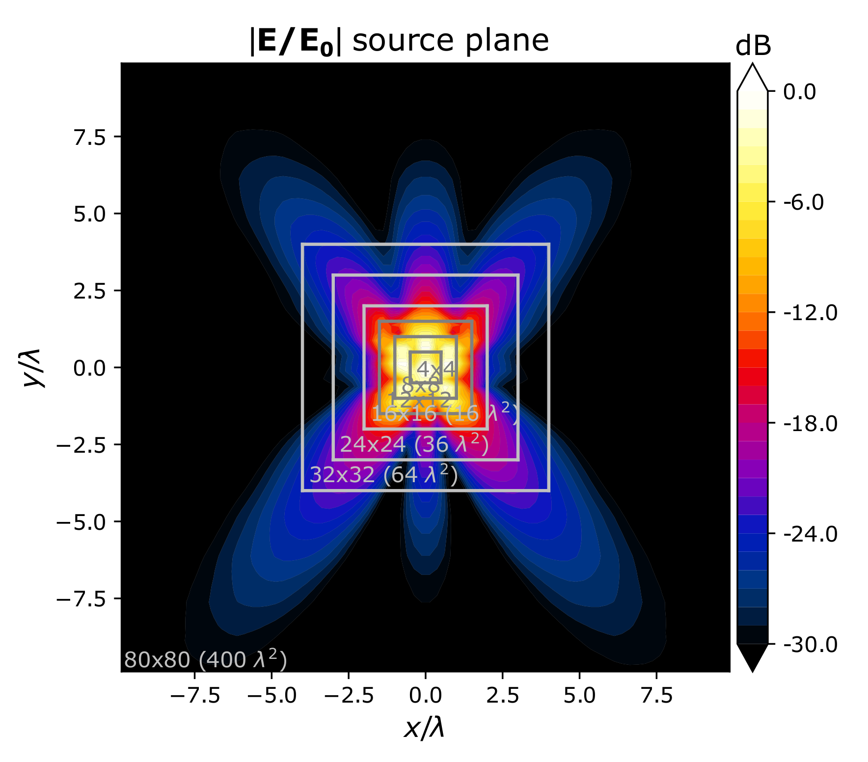
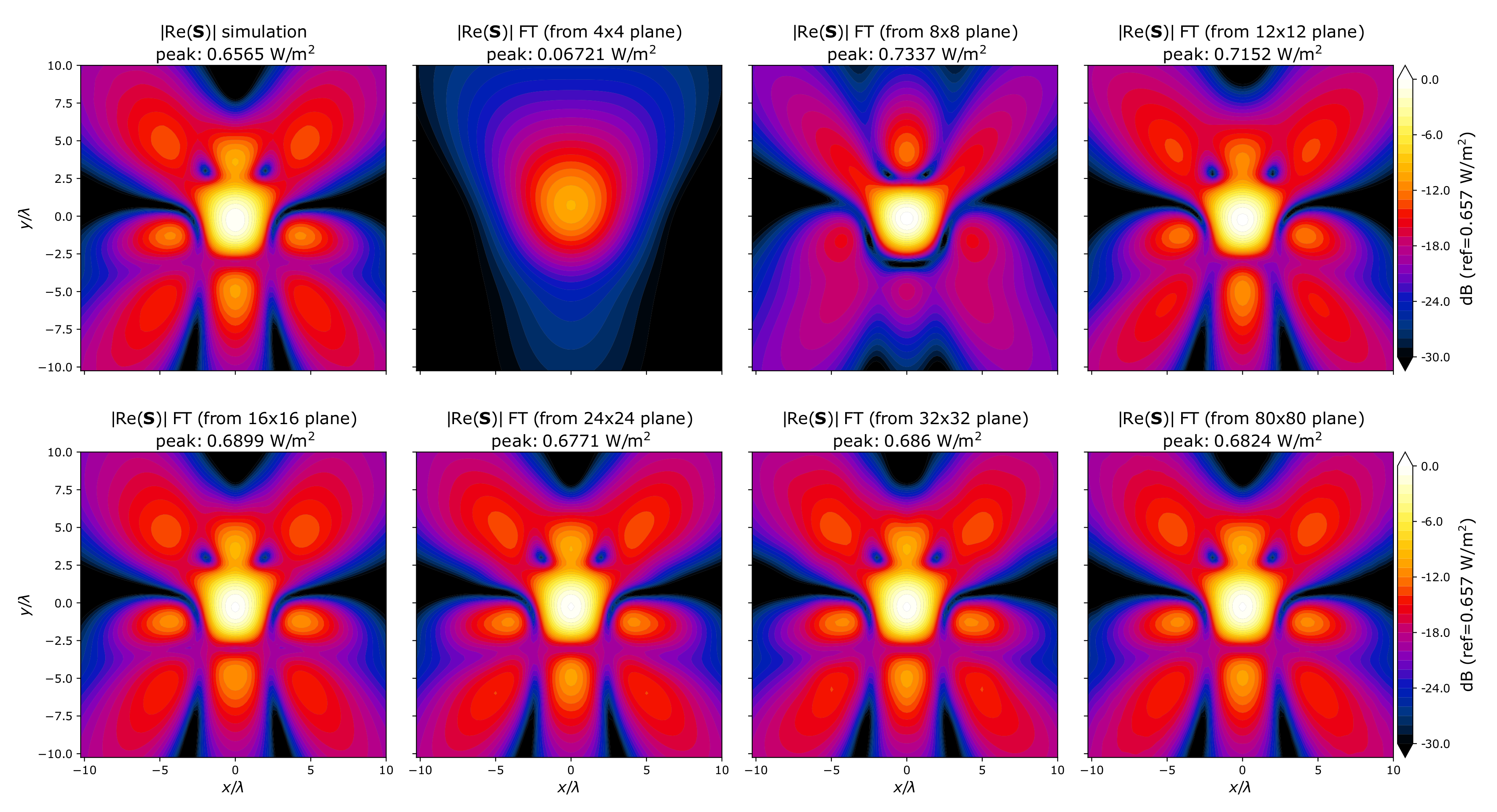
Simulated equivalent currents $\mathbf{M}$ were computed from simulations using (1). Phase reconstruction was omitted in this case to reduce the number of dependent variables and to avoid correcting model inaccuracies by deviating from the actual phases. FT was then applied on a large range of plane sizes. An example of different plane sizes used as planes of equivalent sources is illustrated in Figure 2. The figure also shows the PD computed using FT to a plane further away than the measurement plane. This illustration qualitatively shows how larger plane sizes result in more accurate reconstruction by FT. As a next step, we investigated the error as function of the ratio of the captured power in the finite plane and the total power in the infinite plane.

To quantify the plane size, we used the ratio of power captured by the plane compared to a very large reference plane. The power was computed by the integral of $Re\left({\mathbf{S}}_z\right)$ over the plane. The reference plane was chosen as $80\times 80$ sample points (with a grid step size of $0.25\lambda$). The plane of equivalent currents was placed at $z_1=2\mathrm{mm}$ and two observation planes were used—one at $z_{\mathrm{obs}}=5\mathrm{mm}$ and one at $z_{\mathrm{obs}}=150\mathrm{mm}$—for all frequencies to cover a range that will likely be relevant for the compliance testing of millimeter-wave consumer devices. Note that when performing the FT from the full reference plane to the observation plane, the deviation in psPD was within 0.4 dB of the simulated value for the antennas operating at and above 30 GHz. This deviation was within 0.6 dB for the antennas operating at 10 GHz. These small deviations are mainly attributed to the FT model, which suffers from certain inaccuracies; e.g., the numerical error arising from the discretization of the surface currents in terms of square pulse basis functions. This error due to model imperfections was not further reduced with increasing plane size. 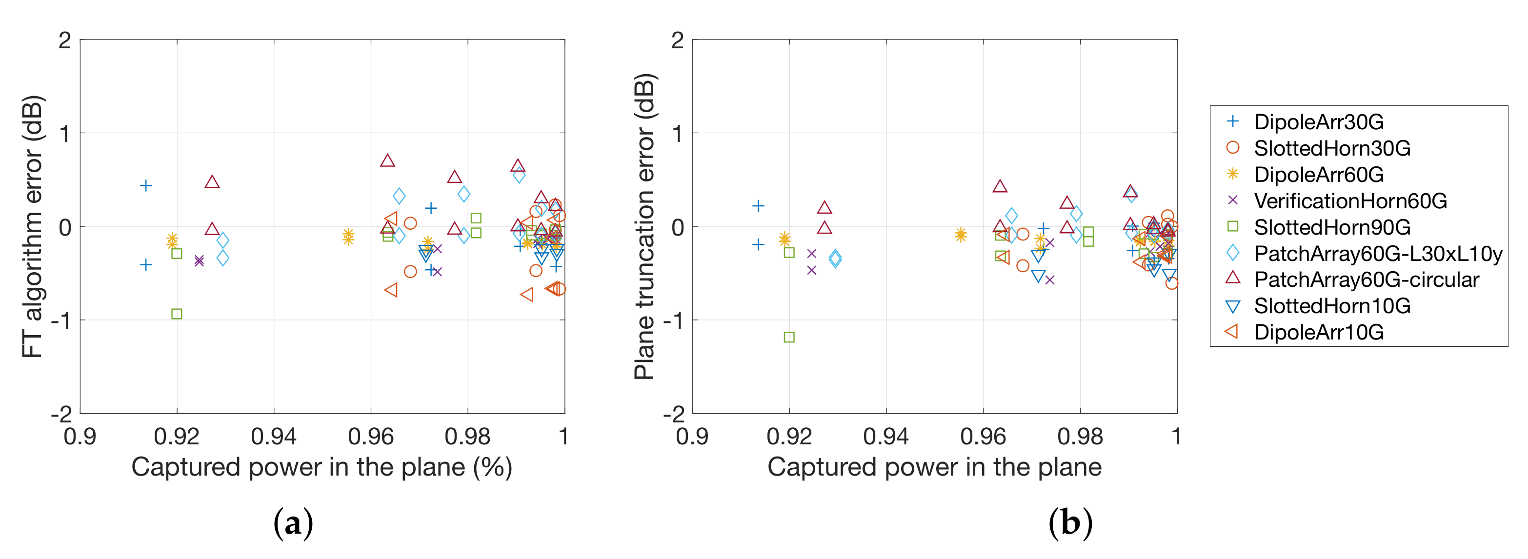In Figure 3, two errors are reported; (i) the error with respect to the real simulated field as the total error of the presented procedure, and (ii) the error with respect to the large reference plane, representing the error caused by plane truncation. The plot of the first error term in Figure 3a shows a convergence to zero with increasing plane size. The plot in Figure 3b depicts the second error term in the absolute power. For planes that capture more than 95% of the whole power of the reference plane, the FT estimate does not change by more than approximately 0.6 dB. For example, the $16\times 16$-plane in Figure 4 captures 99.4% of the power of the $80\times 80$-plane.

The results reported in this section were obtained with simulated equivalent surface currents. They represent a conservative bound for the required plane size when currents are obtained from amplitude measurements and phase reconstruction, as described in Section 2. As the phase reconstruction uses the second and third measurement plane, some modeling errors due to overly small plane sizes are compensated partially by the inverse source reconstruction. This was verified by considering phase reconstruction in the calculations; the resulting dependence on plane size was less pronounced, and planes which captured 99.5% yielded results that could not be substantially improved by larger planes.

6. Algorithm Evaluation

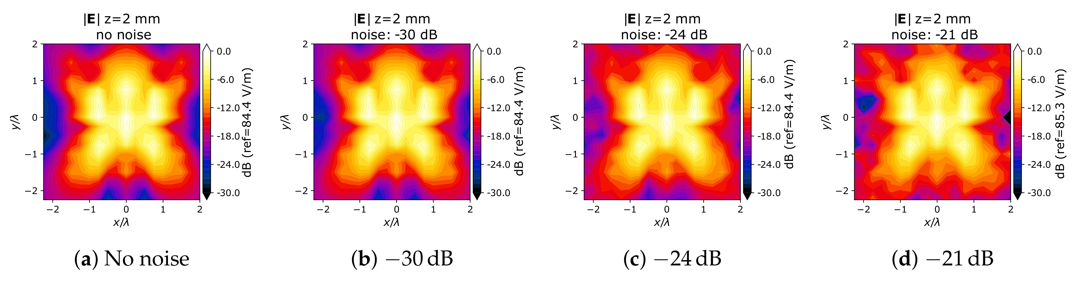
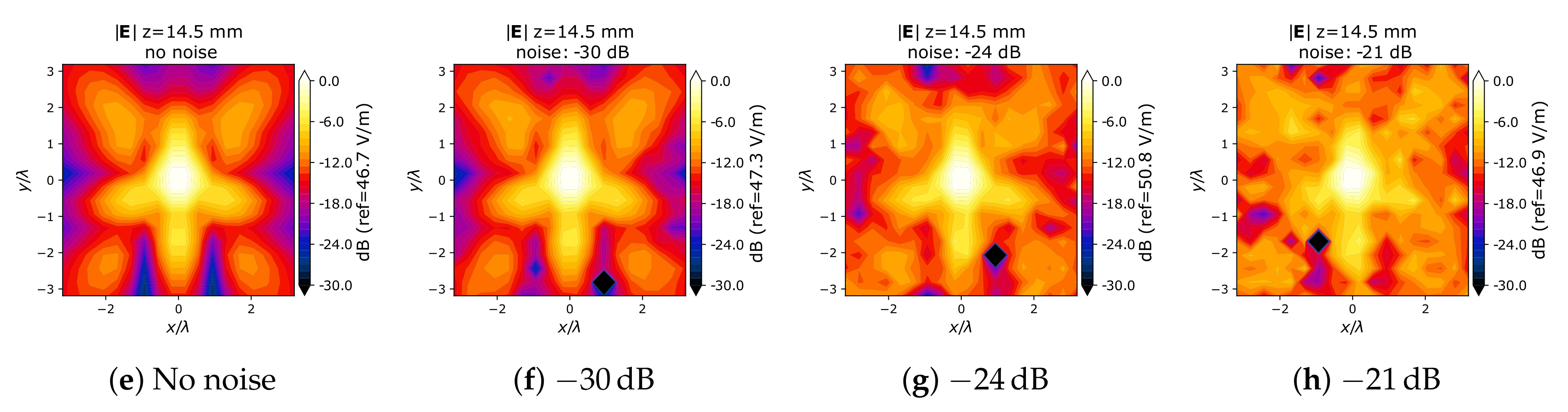
To emulate the measurement data, the simulated E-field vector radiated by the antennas presented in Section 3 was sampled at the location of a virtual EUmmWVx-probe. The sampled field vector was then projected on the plane of sensors integrated in the EUmmWVx-probe, meaning that the components characterized by the field probe were correctly extracted from the simulations. Next, the amplitude was squared, thereby removing phase information, as would be the case for real measurements. To model measurement noise, Gaussian noise was added to the squared E-field amplitudes on the emulated sensors; the standard deviation of this noise was quantified relative to the peak E-field amplitude over the whole measurement plane at 2 mm (in dB). For example, a noise level of −20 dB means the standard deviation of the noise is 10% of the peak E-field signal. The investigated noise levels ranged from −30 dB to −18 dB, in addition to the case without noise.

For the reference fields, the FDTD results including full phase information were used. The first and second measurement planes were placed at $2\mathrm{mm}$ and at $2\mathrm{mm} +0.25\lambda$ from the AUT plane, where the recommended plane separation distance was used from the PTP-algorithm [21]. The size of the measurement plane was chosen based on the results of Section 5 so that at least 99.5% of the power was captured by the plane, which led to plane sizes ranging from $18\times 18$ to $30\times 30$ samples. The grid step size was $0.25\lambda$ (except for the 10 GHz antennas at 2 mm distance, where it was $0.15\lambda$).

The PTP algorithm [21] yielded an initial estimation for ${\mathbf{M}}_{x,0}$ and ${\mathbf{M}}_{y,0}$. The location and dimensions of the third measurement plane were optimized by applying (2) on this initial estimate of ${\mathbf{M}}_{x,0}$, ${\mathbf{M}}_{y,0}$ to obtain a preliminary estimate of the field on the third plane (evaluated on a $128\times 128$ grid). The location and dimension of the “measured” third plane were then chosen to cover the field up to −18 dB of the peak of the preliminary estimate.

The full reconstruction pipeline was run on these data, including reconstruction of the polarization ellipses by means of [28] from the E-field amplitude projected on the sensors, computation of equivalent surface currents at the measurement plane using an additional third measurement plane according to (4), and forward transformation to an evaluation surface by means of (2). Figure 5 shows the magnitude of the generated E-field on the first and third measurement plane used in (4) for different noise levels. FT results were compared to reference values extracted from simulation by means of (7). Finally, the mean and standard deviation over 20 simulations (corresponding to 20 different samplings of random noise) were computed.

7. Simulation Results

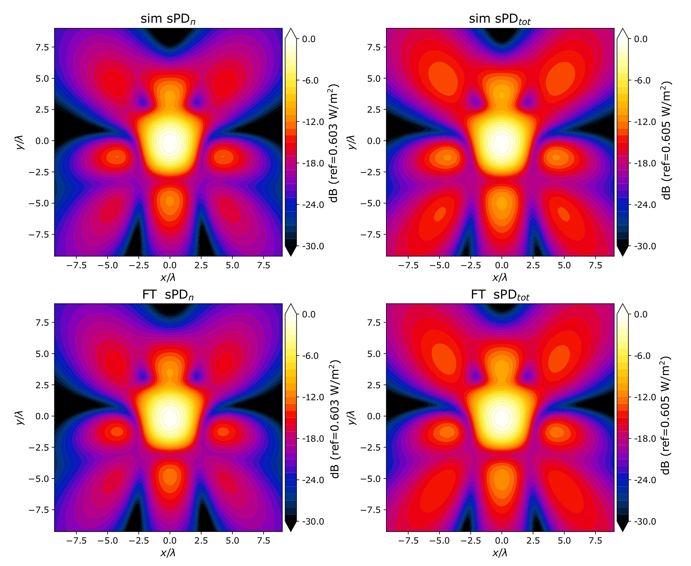
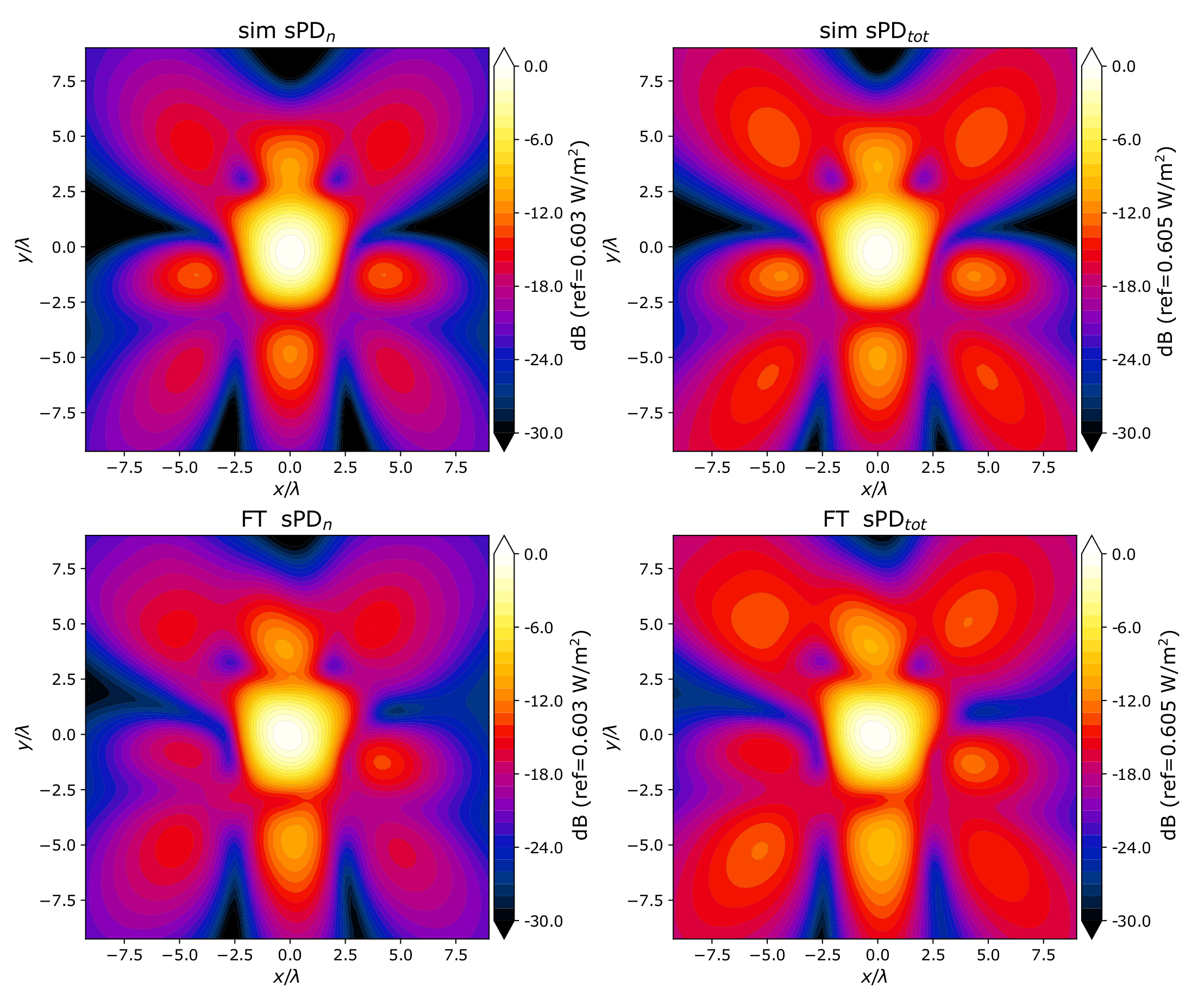
An example of the spatial-average power density (sPD) over 1 cm${}^2$ resulting from a FT to 50 mm distance in the case without noise (Figure 5a,e) is depicted in Figure 6. It shows that the field distribution is reconstructed with only minimal distortions. When noise is added to the emulated measurements–in this example, at a level of −24 dB as described in Section 6 (Figure 5c,g)—the field gets distorted visibly, as can be observed in Figure 7; the error in the ${psPD}_{tot}$ in this example is −0.08 dB without noise and −0.53 dB with −24 dB noise.

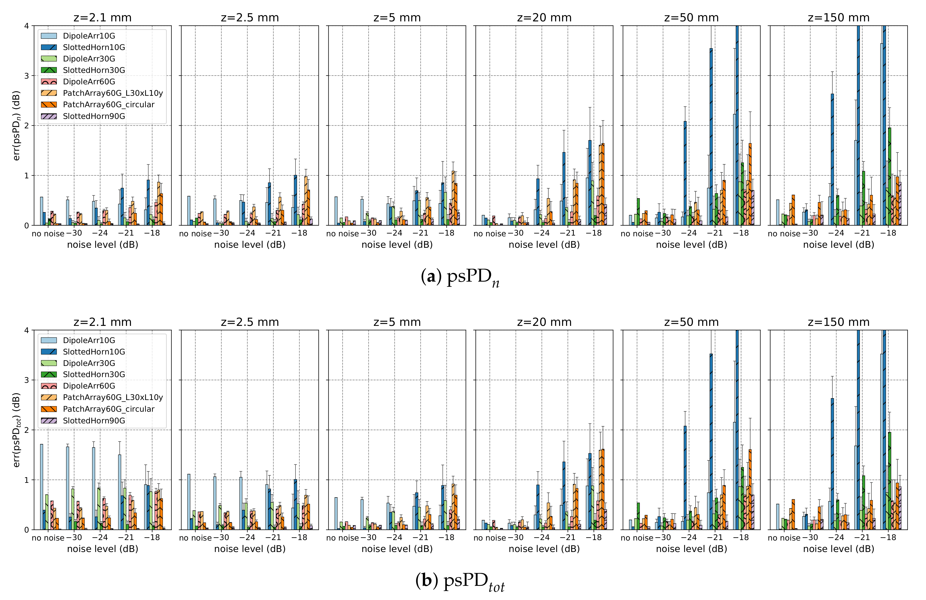
The quantitative results for all antennas are shown in Figure 8. 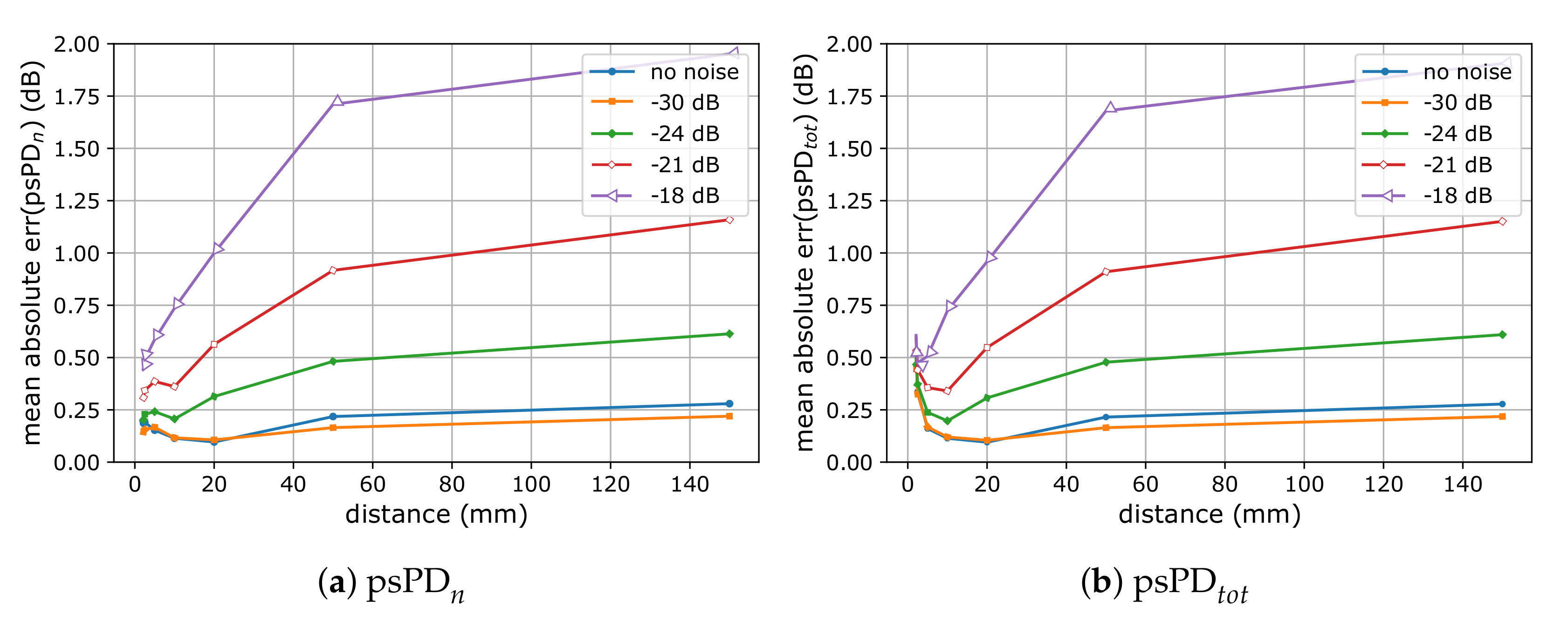For all antennas operating at 30 GHz and above, up to a noise level of −24 dB, the mean absolute error in the psPD flux crossing surface A, ${psPD}_n$, is below 0.61 dB for all distances, ranging from very close (2.1 mm, corresponding to 100 $\mathsf{\mu }\mathrm{m}$ or $\lambda /100$ at 30 GHz distant from the plane of equivalent currents) to far (150 mm, or $45\lambda$ for 90 GHz). The average absolute error over all antennas is shown in Figure 9. It can be seen that, for small distances (2.1, 2.5 and 5 mm), the results are similar for the different noise levels up to −21 dB. For high noise levels, the error increases, especially for larger distances (50 mm and 150 mm). This may be attributed to phase reconstruction errors, which become more apparent at larger distances. For distances extremely close to the plane of equivalent currents, as seen for 2.1 mm, the error in the spatial-averaged norm of the Poynting vector ${psPD}_{tot}$ is larger than ${psPD}_n$, up to approximately 0.8 dB (for 30 GHz and above), even for very low noise levels. This discrepancy (also visible in Figure 8) is likely due to the reactive components that contribute to ${psPD}_{tot}$; they are more difficult to reconstruct than the mostly propagating components contained in ${psPD}_n$. From 5 mm and larger distances, no substantial difference can be observed between the two error metrics. The marginally higher error for the no noise case compared with the −30 dB noise case shows that there are other error sources, such as errors in the phase reconstruction algorithm and numerical errors originating from the expansion of magnetic current in terms of step functions.

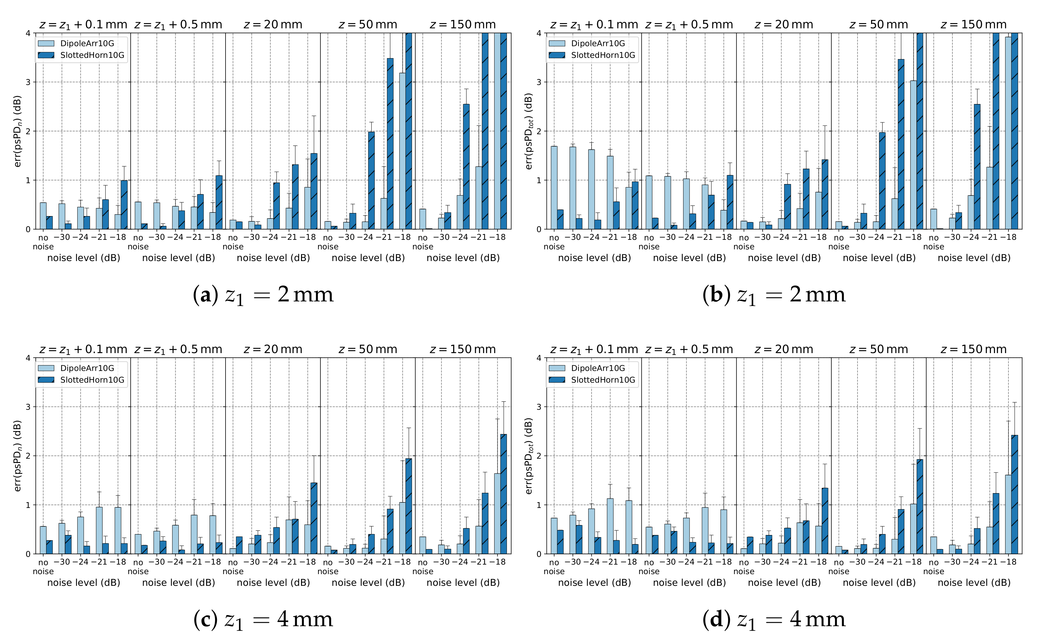
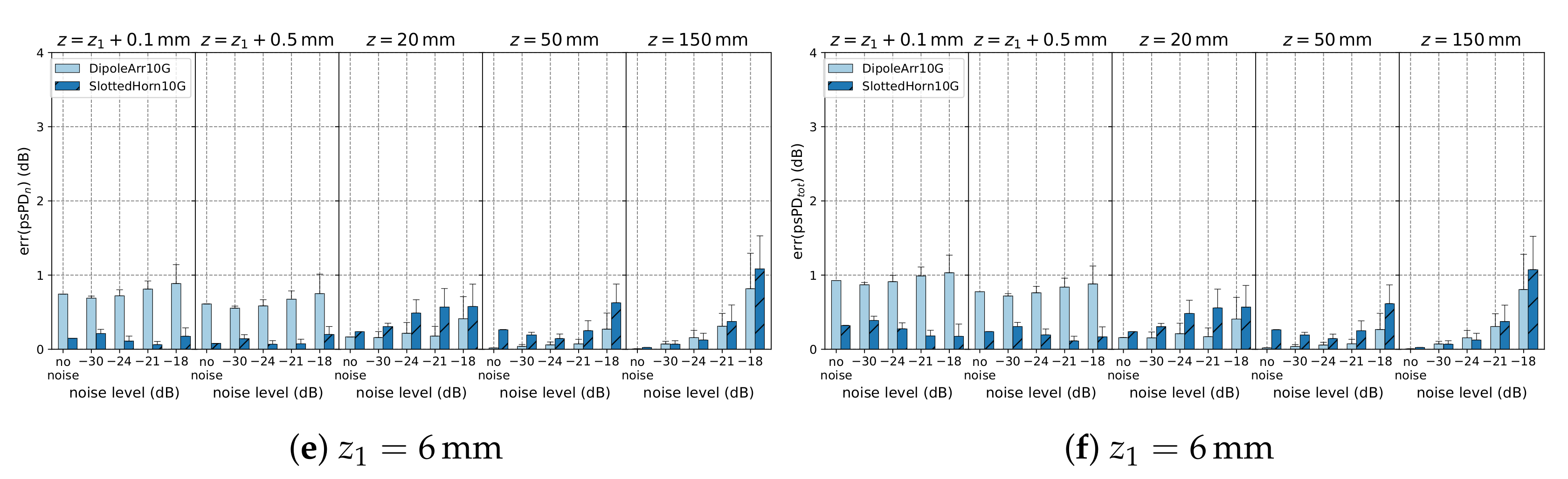
It is apparent that the errors for the antennas operating at 10 GHz are relatively high. This can be explained by the very close distance of the plane of equivalent currents $z_1$, 2 mm from the AUT, which corresponds to $\lambda /30$. To investigate this in more detail and to illustrate how the problem is resolved at greater distances, different distances of $z_1$, i.e., 2 mm, 4 mm and 6 mm, were investigated. These correspond to the same electrical distance as the measurement of a 10 GHz, 20 GHz or 30 GHz antenna at 2 mm distance. As evaluation distances, short distances to the closest plane were used ($z_1+0.1\mathrm{mm}$, $z_1+0.5\mathrm{mm}$), in addition to the distances 20 mm, 50 mm and 150 mm. The results are depicted in Figure 10. It can be observed that, even for a distance $z_1$ of 4 mm, the mean error levels drop below 0.92 dB for noise levels of −24 dB or smaller, even for the FT evaluation distance of 4.1 mm, which is extremely close to the plane of equivalent currents $z_1$ (corresponding to a distance of $\lambda /300$ from $z_1$). For FT evaluation distances further away ($\lambda /60$ from $z_1$ and further), the mean errors are below 0.76 dB. Note that a 4 mm distance at 10 GHz corresponds to the same electrical distance as 2 mm at 20 GHz.

8. Validation with Measurements

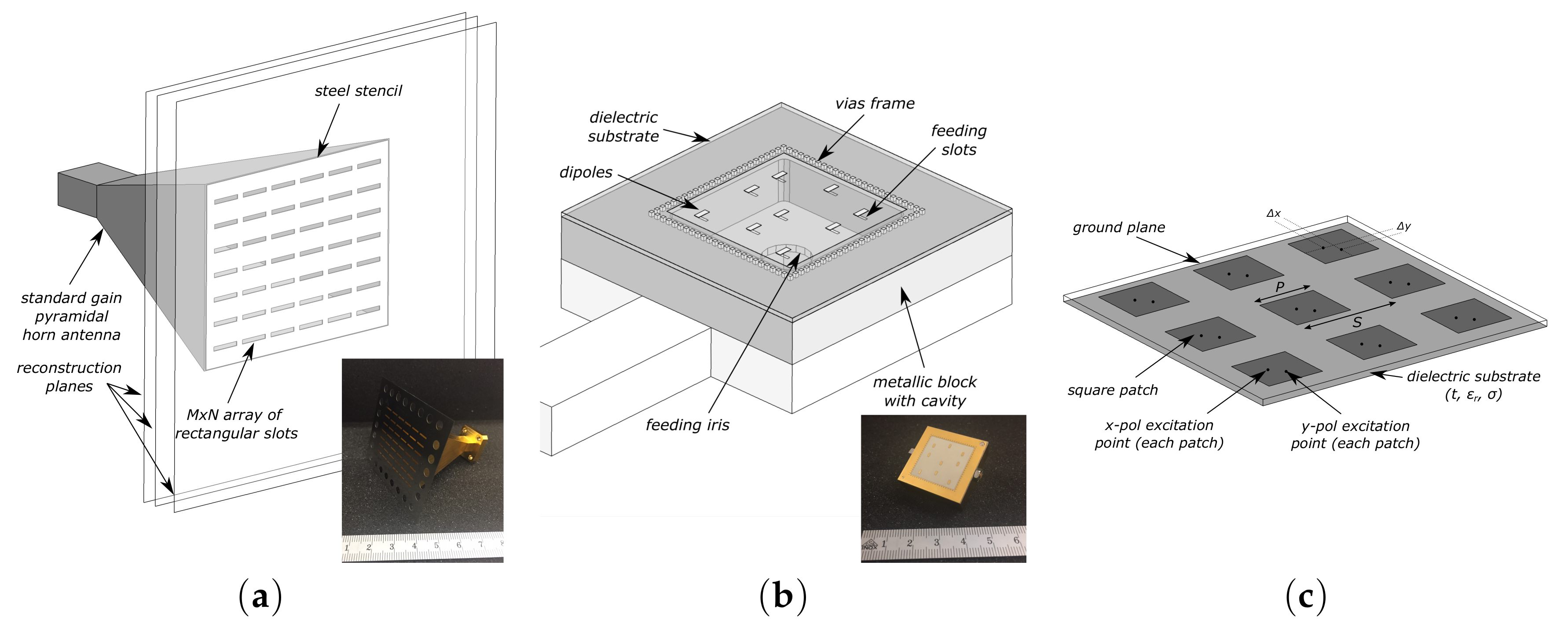
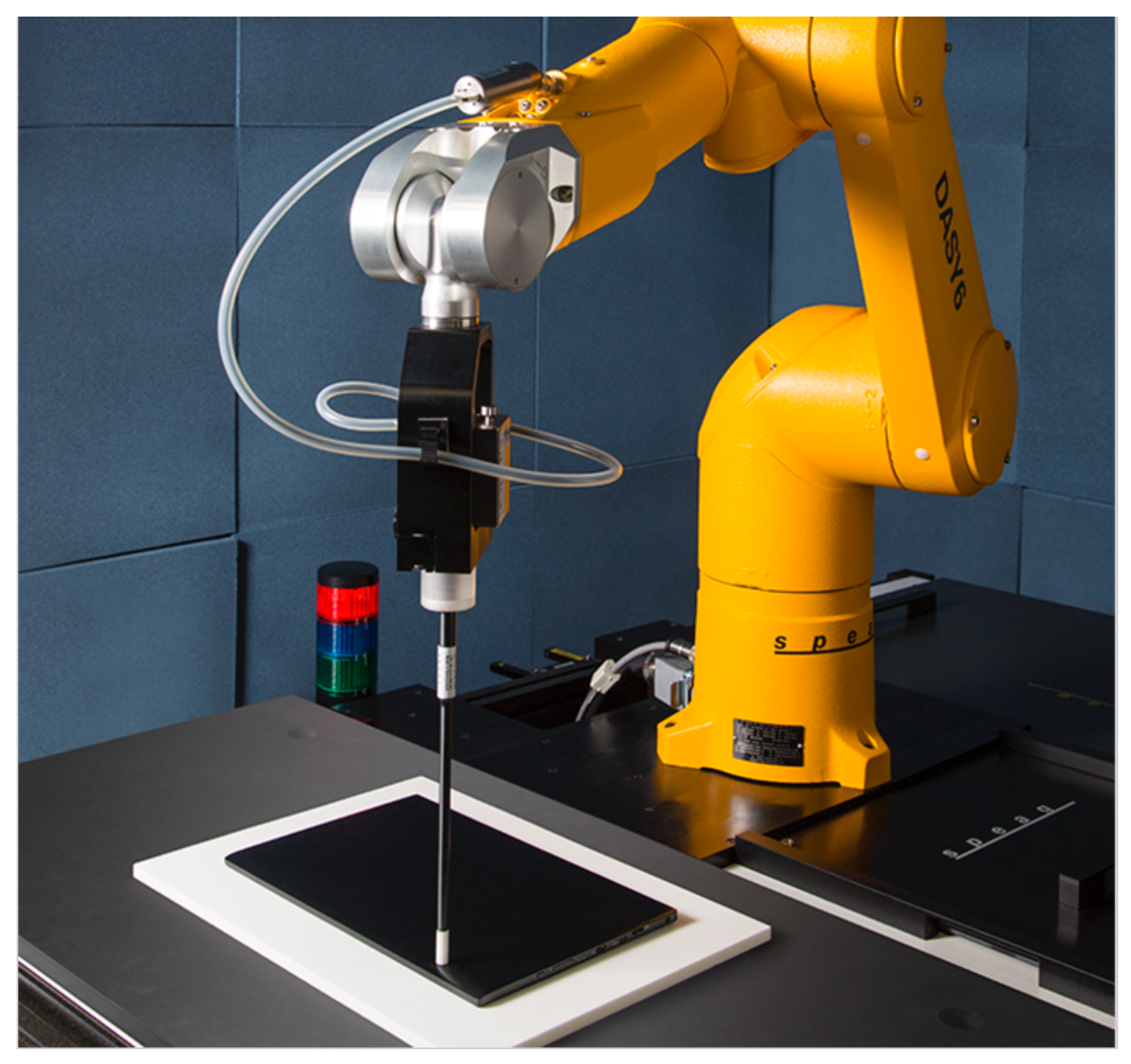
To validate the new phase reconstruction method with measurements, a subset of the simulated antennas was measured, namely the cavity-fed dipole array at 30 GHz and at 60 GHz and the horn loaded with a slot array at 30 GHz and at 90 GHz (see Figure 1). These measurements are performed using the cDASY6 mmWave module (EUmmWVx) [20] shown in Figure 11.

The EUmmWVx probe is based on the pseudo-vector probe design, which not only measures the field magnitude but also derives its polarization ellipse. This probe concept also has the advantage that the sensor angle errors or distortions of the field by the substrate can be largely nullified by calibration. This is particularly important as, at these very high frequencies, field distortions by the substrate are dependent on the wavelength. The design entails two small 0.8 mm dipole sensors mechanically protected by high-density foam, printed on both sides of a 0.9 mm wide and 0.12 mm thick glass substrate. The body of the probe is specifically constructed to minimize distortion by the scattered fields. The probe consist of two sensors with different angles arranged in the same plane in the probe axis. Three or more measurements of the two sensors are taken for different probe rotational angles to derive the amplitude and polarization information. These probes are the most flexible and accurate currently available for measuring field amplitude. Their design allows measurements at distances as small as 2 mm from the sensors to the surface of the device under test (DUT). The closest measurement plane (corresponding to the plane of equivalent currents) was placed at a distance $z_1=2\mathrm{mm}$ from the AUT and the procedure for phase reconstruction and FT was the same as described in Section 2. The radiation efficiency of the antennas was determined using the ${psPD}_n$ averaged over 1 cm${}^2$ at a large distance (i.e., at 50 mm).

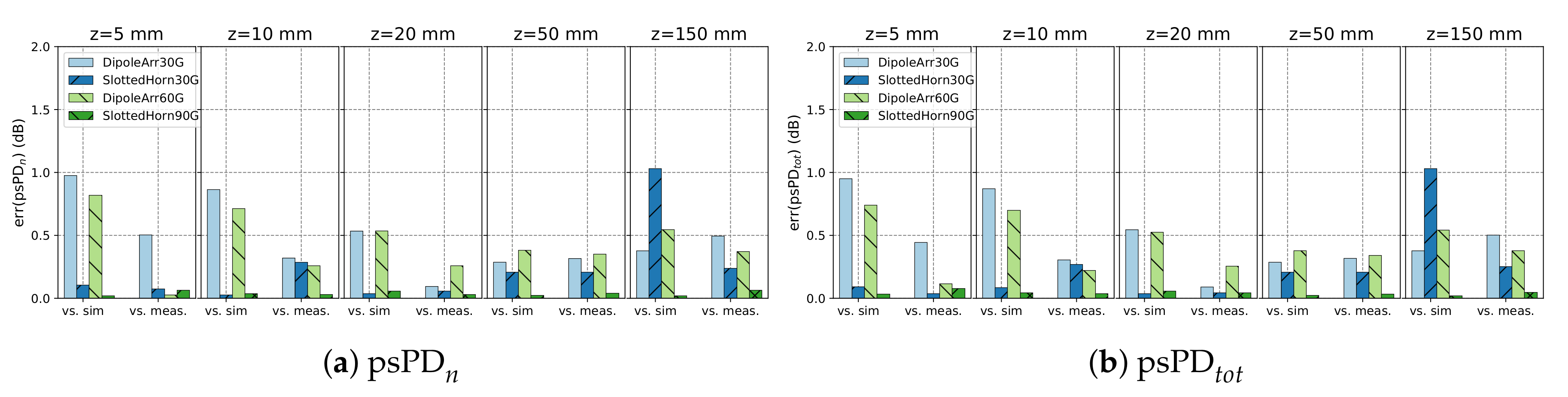
The FT was evaluated at distances of 5, 10, 20, 50 and 150 mm from the AUT, and the resulting psPD was compared to two different reference values: one was a measurement at the respective distance and the other was the simulated value. The noise levels in the measurements were below $-30$ dB; note that in the simulation study (Section 7), deviations from reference values were within approximately 0.5 dB for these noise levels.

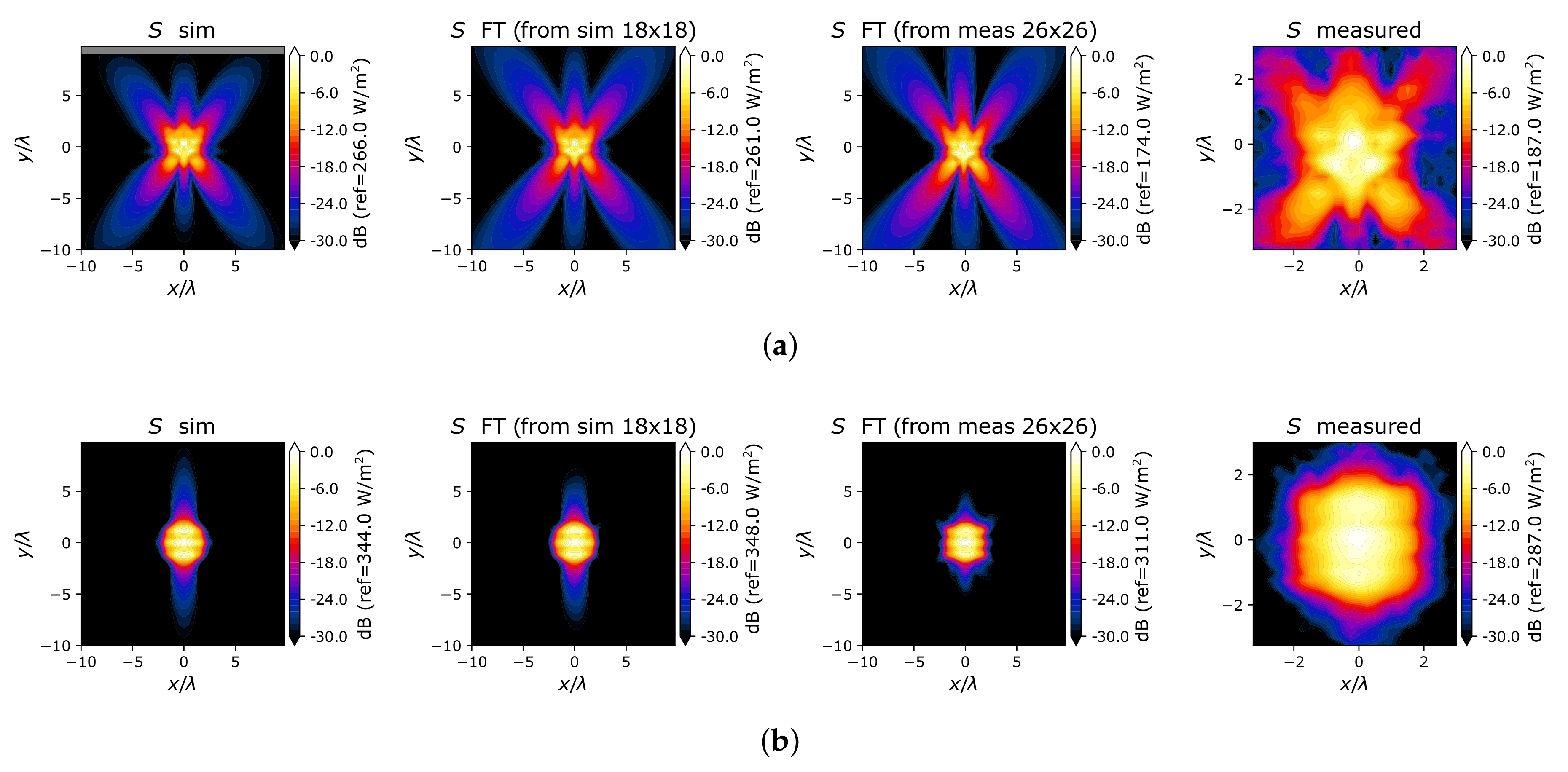
The results are shown in Figure 12. It can be seen that, when comparing FT results to measurements, all results are within 0.6 dB of the measurement reference. This is well within the expected deviations from the simulation study, especially when considering that only Gaussian noise on the sensors was modeled without considering other effects such as positioning errors or sensor isotropy. As an example, the simulated, measured and reconstructed radiation patterns at a 5 mm distance from the AUT are illustrated in Figure 13 for the two cases of the cavity-fed dipole array and horn antenna loaded with slot arrays.

In comparison to the simulation reference, deviations are within 1.1 dB. These larger deviations compared to measurements may be attributed to modeling uncertainty (agreement between exposure setup and simulated setup).

9. Summary and Conclusions

The paper presents a new method for reconstructing the EMF in the full half-space above a measurement plane as close as 2 mm from the AUT plane by using the well-known field integral equations and SPEAG’s EUmmWVx probe [20]. The method was verified using eight antennas developed to validate measurement systems covering the frequency range from 10–90 GHz. These antennas were selected as they were developed with the intention to pose a challenge for the measurement systems at close distances to the antenna structure. In addition, different noise levels were investigated, with each modeled according to the physical conditions inside the EUmmWVx probe. Finally, the approach was validated with measurements of four different antennas.

The results show that deviations between reconstruction using FT and simulations were within approximately 0.7 dB for the evaluated distances, ranging from 2.1–150 mm from the antenna for noise levels of −24 dB and smaller. These deviations are marginally higher for the antennas operating at 10 GHz, where a measurement distance of 4–6 mm, corresponding to $0.14\lambda -0.2\lambda$, was required to achieve similar error levels. When comparing FT from measurements close to AUT with direct measurements at the same distance, the results were within 0.6 dB for all four tested antennas.

The results demonstrate that the new FT method is applicable for compliance assessment and can lead to substantial time savings since the number of required measurements can be dramatically reduced. For example, in cases in which exposure measurements on six surfaces are required, fields on 12 planes should be measured so that, after phase reconstruction, the obtained phasors on the measurement planes return the radiated power. Using the developed algorithm, measurement on one surface is sufficient for obtaining the phasors in the near-field domain and subsequently propagating them to all other five surfaces. Moreover, the possibility of placing the reconstruction surface very close to the AUT reduces the required number of measurements dramatically. For instance, for the example SlottedHorn10G, a grid of 8 × 8 measurement points with 0.25 ${\lambda }_{10\mathrm{GHz}}$ resolution was enough to capture 98% of the radiated power. A 12 × 12 grid with 0.25 ${\lambda }_{30\mathrm{GHz}}$ resolution captures 97% of the radiated power in the DipoleArr30G example, and in the PatchArray60G_circular case, a 10 × 10 grid suffices to sample 96% of the radiated power.

This approach results in a very fast demonstration of safety when the device is operating at the head. All assessments are limited to one surface at the closest distance, with the advantage that it is the smallest surface and has the best signal-to-noise ratio. As a rule of thumb, measuring one plane took roughly half an hour to one hour on a cDASY6 system (SPEAG, Zürich, Switzerland) for the investigated antennas; on a state-of-the-art desktop computer, phase reconstruction took few minutes, and evaluating different planes using FT only took a few seconds.