Abstract
Monitoring vegetation cover is an essential parameter for assessing various natural and anthropogenic hazards that occur at the vicinity of archaeological sites and landscapes. In this study, we used free and open access to Copernicus Earth Observation datasets. In particular, the proportion of vegetation cover is estimated from the analysis of Sentinel-1 radar and Sentinel-2 optical images, upon their radiometric and geometric corrections. Here, the proportion of vegetation based on the Radar Vegetation Index and the Normalized Difference Vegetation Index is estimated. Due to the medium resolution of these datasets (10 m resolution), the crowdsourced OpenStreetMap service was used to identify fully and non-vegetated pixels. The case study is focused on the western part of Cyprus, whereas various open-air archaeological sites exist, such as the archaeological site of “Nea Paphos” and the “Tombs of the Kings”. A cross-comparison of the results between the optical and the radar images is presented, as well as a comparison with ready products derived from the Sentinel Hub service such as the Sentinel-1 Synthetic Aperture Radar Urban and Sentinel-2 Scene classification data. Moreover, the proportion of vegetation cover was evaluated with Google Earth red-green-blue free high-resolution optical images, indicating that a good correlation between the RVI and NDVI can be generated only over vegetated areas. The overall findings indicate that Sentinel-1 and -2 indices can provide a similar pattern only over vegetated areas, which can be further elaborated to estimate temporal changes using integrated optical and radar Sentinel data. This study can support future investigations related to hazard analysis based on the combined use of optical and radar sensors, especially in areas with high cloud-coverage.
1. Introduction
Various hazards, both anthropogenic and natural, can affect cultural heritage landscapes, sites, and monuments. These hazards include fires, landslides, soil erosion, agricultural pressure, and urban expansion [1,2,3,4,5]. In the recent past, several publications have demonstrated the benefits of Earth Observation sensors, providing wide and systematic coverage over archaeological sites providing systematic observations at medium and high-resolution images [6,7,8,9,10]. In addition, access to archival imageries is a unique advantage of Earth Observation repositories, allowing for the analysis of the temporal evolution of a hazard [11,12,13].
Nowadays, open and freely distributed satellite images, both radar and optical, have become available due to the European Copernicus Programme [14]. The Sentinel sensors, with increased revisit time and medium-resolution satellite images, can be downloaded through specialized big data cloud platforms such as the Sentinel Hub [15]. These kinds of services provide radiometric and geometric corrected Bottom of Atmosphere (BOA) reflectance bands of the Sentinel-2A,B sensors, as well as orthorectified gamma 0 VV and VH radar images of the Sentinel-1 Synthetic Aperture Radar (SAR) sensor (ascending and descending). Beyond these calibrated images, other ready products are available for further re-use, like optical and radar vegetation indices (e.g., the Normalized Difference Vegetation Index—NDVI and the Radar Vegetation Index—RVI). Pseudo-colour composites can be readily displayed in the Sentinel Hub service, thus enhancing urban and agricultural areas, while classification products are also provided.
Monitoring vegetation dynamics and long-term temporal changes of vegetation cover is of great importance for assessing the risk level of a hazard [16,17]. For instance, the decrease of vegetation cover, as a change to either the NDVI or RVI, can be a signal for land-use change and a result of the urbanization sprawl phenomenon [18,19,20,21]. In contrast, an increase in the vegetation cover, beyond the phenological cycle of the crops, can be a warning of agricultural pressure [22,23,24]. Similarly, vegetation indices are input parameters for studying other hazards such as soil erosion and fires [25,26]. For soil erosion, vegetation cover is linked with the land cover factor, which indicates the proportion of water that runs on the ground surface. A decrease of vegetation in a concise period can be an indicator of a fire event. For instance, Howland et al. [27] used the NDVI to estimate the soil erosion by water, based on the Revised Universal Soil Loss Equation. In Burry et al.’s study [28], multi-temporal vegetation indices analysis was used to map fire events and help to understand and interpret archaeological problems related to past settlement patterns or environmental scenarios. However, in many cases, optical and radar vegetation indices are applied separately with no synergistic use, thus minimizing the full potentials of existing Earth Observation systems.
In this study, we aim to investigate the use of optical and radar images, from freely available and open-access datasets, like the Sentinel-1 and Sentinel-2 sensors for estimating the proportion of vegetation cover. The investigation was supported by other open access services, namely the crowdsourced OpenStreetMap initiative. OpenStreetMap is an editable geo-service with more than 6 million users all around the world. These ground-truthed datasets can be used to train the medium-resolution Sentinel images, for detecting fully vegetated and non-vegetated areas. Additionally, Google Earth, a free platform that provides systematic snapshots of high-resolution optical satellite data, can be used as an evaluation of the OpenStreetMap datasets. In short, the current study aims to investigate cross-cutting applications among the Copernicus Sentinel-1 and Sentinel-2 sensors, core services, and other third-party data for the estimation of the proportion of vegetation cover in the vicinity of archaeological sites.
2. Case Study Area
The case study area is located on the western part of Cyprus, at the Paphos district (Lat: 34.76°, Long: 32.41°, WGS 84 projection). This area holds important open-air archaeological sites and monuments like the UNESCO enlisted archaeological sites of “Nea Paphos” and “Tombs of the Kings” while several historical buildings are found at the Centre of Paphos town. More information regarding the archaeological context of the area can be found in [29]. Figure 1 indicates the area of interest (zones a and b), while a land-use/land-cover map from the CORINE 2018 program [30] is displayed in the background. The CORINE Land Cover inventory was initiated in 1985 and regular updates have been produced in 2000, 2006, 2012, and 2018. It consists of an inventory of land cover with 44 classes [30].
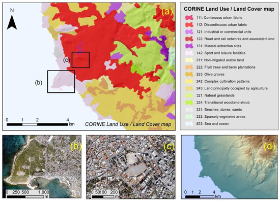
Figure 1.
The selected case study area located in the western part of Cyprus. The various thematic classes from the Corine Land Use Land Cover 2018 dataset [13] over the area of interest are shown in (a), while some high-resolution aerial orthophotos provided by the Department of Land and Surveyors (scale 1:5000) are shown in (b) (archaeological site of Nea Paphos) and (c) (historical Centre of Paphos town). (d) shows the elevation of the area.
The landscape of Paphos is threatened by various natural and anthropogenic hazards such as soil erosion [31], urban expansion [32] and fires [33]. Several studies have been performed in the past on these hazards. For instance, in [32], Agapiou et al. reported an increase of more than 300% in the urban areas in a period of 30 years, indicating the dramatic and sudden landscape changes in the surroundings of these important archaeological sites. Moreover, Panagos et al. [34] reported this area to have high erodibility due to water.
3. Materials and Methods
In this section, the overall methodology, as well as the datasets used for the needs of the current study, are presented. The various equations for estimating the proportion of vegetation and the layers of information are also presented.
3.1. Methodology
For the needs of the study, various sources were used (Figure 2). The first source of information regards the optical and radar Sentinel datasets, acquired over the area of interest. The second source of information considers the Sentinel ready products from the Sentinel Hub service. The third component refers to the crowdsourced vector geodata manually digitized by several users of the area of interest, available at the OpenStreetMap service [35]. The accuracy assessment of the OpenStreetMap service is still debated by researchers while several examples of this service blended with remote sensing can be found in the literature [36,37,38]. Finally, the compressed red-green-blue (RGB) high-resolution optical data from the Google Earth platform are used for validation purposes.
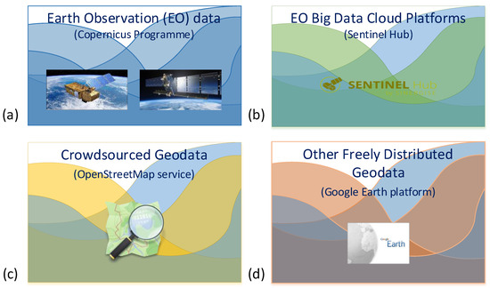
Figure 2.
A schematic representation of the four “layers” of information used in this study: the Earth Observation Sentinel-1 and Sentinel-2 images (a), the Sentinel Hub, an Earth Observation big data cloud platform (b), crowdsourced geodata from OpenStreetMap (c) and the Google Earth platform (d).
Through the Sentinel Hub service, radar and optical Sentinel images were retrieved (see more details below). Beyond the calibrated bands from both sensors, additional products were generated. The NDVI and the RVI were processed using Equations (1) and (2):
where the ρNIR and ρRED refer to the reflectance value (%) of the near-infrared and red bands of the Sentinel-2 sensor (namely using the band 8 and band 4), while the VV and VH refer to the polarization bands of the Sentinel-1 sensor, it should be mentioned that the estimation of the RVI was based upon a custom script available with the Sentinel-Hub services at [39]. As mentioned in [39], an equivalent to the degree of polarization (DOP) is calculated as VV/(total power), where the latter is estimated as the sum of the VV and the VH polarization of the Sentinel sensor. The DOP is utilized to obtain the depolarized fraction as m = 1 – DOP and it can range between 0 and 1. For pure or elementary targets this value is close to zero, whereas for fully random canopy (at high vegetative growth), it reaches close to 1. This m factor is multiplied with the vegetation depolarization power fraction (4 × VH)/(VV + VH). The m factor is modulated with a square root scaling for a better dynamic range of the RVI.
NDVI = (ρNIR – ρRED)/(ρNIR + ρRED),
RVI = (VV/(VV + VH))0.5 (4 VH)/(VV + VH),
From optical and radar vegetation indices, the proportion of vegetation can be retrieved. In our study, two different models were applied for both optical and radar datasets:
where vegetation index veg (NDVI veg and RVI veg) and non-vegetation index (NDVI non-veg. and RVI non-veg.) represent the vegetated and non-vegetated pixels of the considered index, respectively, vegetation index max (NDVI max and RVI max) and vegetation index min (NDVI min and RVI min) represent the maximum and minimum histogram value of the vegetation image.
Pv1-radar = (RVI - RVI non-veg.)/(RVI veg - RVI non-veg.),
Pv1-optical = (NDVI - NDVI non-veg.)/(NDVI veg - NDVI non-veg.),
Pv2-radar = [(RVI - RVI min)/(RVI max - RVI min)]0.5
Pv2-optical = [(NDVI - NDVI min)/(NDVI max - NDVI min)]0.5
It is evident, therefore, that the selection of vegetated and non-vegetated regions is of great importance for the correct estimation of the proportion of vegetation cover. For this reason, the crowdsourced OpenStreetMap was used as a training area for the equations mentioned above, once these vector polygons have been confirmed from the Google Earth high-resolution products. Once these sites have been selected, the results from the optical and radar sensors using Equations (3)–(6) were retrieved. A comparison between the optical and the radar sensors separately (namely the results from Equation (3) against the results from Equation (4), and the results from Equation (5) with the results from Equation (6)) was performed.
3.2. Datasets
For the aims of the current study, radar Sentinel-1 and optical Sentinel-2 images were downloaded through the EO Browser of the Sentinel Hub service [15]. The characteristics of these images are shown in Table 1 and Table 2.

Table 1.
Characteristics of the Sentinel-1 (Interferometric Wide Swath (IW)), sensor.
Table 2.
Characteristics of the Sentinel-2 sensor.
In particular, a radar Sentinel-1 image in Interferometric Wide Swath (IW), acquired on 12 May 2020 was processed. In addition, a Sentinel-2 image with processing level L2A (orthorectified BOA) and limited cloud-coverage acquired on 13 May 2020 was used. Figure 3 visualizes the Sentinel-1 and -2 images as well as other ready products available from the Sentinel Hub service. It should be mentioned that all these images were downloaded in high-resolution format (which corresponds to 10-m spatial resolution per pixel) and in a 32-bit tiff image format. Figure 3a,b display the orthorectified Sentinel-1 VH and VV gamma 0 respectively, while Figure 3c shows the Sentinel-1 SAR urban visualization product. The SAR urban product is an RGB pseudo-composite, whereas the combination VV-VH-VV is used for the RGB composite. The Radar Vegetation Index (RVI) is displayed in Figure 3d. Figure 3e–i refer to products and bands of the optical Sentinel sensor as follow: Figure 3e,f show the Sentinel-2, BOA Band 5 (red-edge) and band 8 (near-infrared) respectively. The Normalized Difference Vegetation Index (NDVI) can be observed in Figure 3g. Figure 3h shows the Sentinel-2 Scene Classification product, which is developed under the Sen2Cor project to support an atmospheric correction module. In addition, monthly Sentinel-1 and Sentinel-2 ready products (RVI and NDVI) were used for over a year (May 2019–May 2020) so as to investigate temporal changes of vegetation growth with these indices.
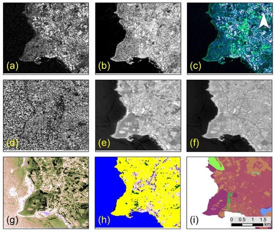
Figure 3.
Sentinel-1 and Sentinel-2 datasets and ready products downloaded from the EO Browser of the Sentinel Hub Service used in this study. (a) orthorectified Sentinel-1, VH polarization, gamma 0, (b) orthorectified Sentinel-1, VV polarisation, gamma 0, (c) Sentinel-1 Synthetic Aperture Radar (SAR) urban visualization product, (d) Sentinel-1 Radar Vegetation Index, (e) Sentinel-2, Bottom-of-Atmosphere (BOA) Band 5, (f) Sentinel-2, Bottom-of-Atmosphere (BOA) Band 8, (g) Sentinel-2, Normalized Difference Vegetation Index (NDVI), (h) Sentinel-2, Scene Classification product, and (i) the OpenStreetMap vector data of the area. The scale for all sub-figures is shown in the right bottom part of the Figure 3.
Furthermore, OpenStreetMap data were retrieved through the QGIS open-access software [40]. In our case study area, various vector data are available for download, as shown in Figure 3i. From these vector polygons, areas characterized as vegetated and non-vegetated were identified and compared with available images from the Google Earth platform.
4. Results
In this section, the overall results are presented. In Section 4.1, the results from the implementation of the optical and the radar vegetation indices are presented, while the proportion of vegetation is estimated and visualized in Section 4.2. The evaluation of these results is finally discussed in Section 4.3.
4.1. Vegetation Indices
As mentioned earlier, the calibrated optical and radar bands were retrieved from the Sentinel Hub platform. Based on the equations provided before Equations (1) and (2) the NDVI and the RVI were estimated (also see Figure 3d–g). The range of these indices is between −1 to +1 for the NDVI while for the RVI the range value is between 0 to +1. With the increase of vegetation cover, the value of both indices increased to +1. At the same time, non-vegetated areas are close to 0 (and negative for the NDVI in water bodies). Since the acquisition period for the Sentinel-1 and the Sentinel-2 images only had a one day difference, it was hypothesized that both indices were obtained at the same phenological status of vegetation. The results from the application of the vegetation indices over the area of interest are depicted in Figure 4. Figure 4a,d,g show the Sentinel-2 true colour composite over the area of interest, the archaeological site of “Nea Paphos” and the historic Centre of the Paphos town, respectively. Likewise, Figure 4b,e,h display the results of the RVI, while Figure 4c,f–i show the results from the NDVI.
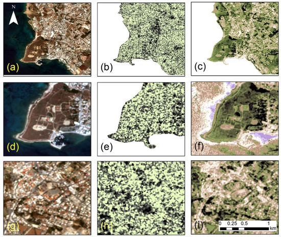
Figure 4.
(a) Sentinel-2 true colour over the area of interest, (b) Radar Vegetation Index (RVI), (c) Normalized Difference Vegetation Index (NDVI), (d) closer look of (a) over the archaeological site of “Nea Paphos”, (e) closer look of (b) over the archaeological site of “Nea Paphos”, (f) closer look of (c) over the archaeological site of “Nea Paphos”, (g) closer look of (a) over the historical Centre of Paphos town, (h) closer look of (b) over the historical Centre of Paphos town, and (i) closer look of (c) over the historical Centre of Paphos town. Vegetated areas are shown with green colour while non-vegetated areas with black colour for the RVI, while for the NDVI vegetation is highlighted with dark green colour.
Vegetated areas as estimated from the RVI (Figure 4b,h) are shown with a green colour while non-vegetated areas are visualized with a black colour. Vegetated areas in the NDVI (Figure 4c,f–i) are highlighted with a dark-green colour and non-vegetated areas with a light-yellow colour. From Figure 4, it is evident that optical products are more easily visually interpreted compared to the radar products, however, this could be explored when optical images are not available, such as the case of high cloud-coverage of the area of interest.
To investigate if any correlation between the NDVI and the RVI values can be established, regression models were applied. Figure 5 shows a scatterplot of 1000 points distributed randomly over the case study area, at different target types, indicating the NDVI and RVI values at the X and Y axis, respectively. As it is shown in this scatterplot, a high variance is observed, indicating that no strong correlation between these two indices can be achieved. This is also aligned with the previous findings, indicating that optical and radar indices do not produce similar findings.
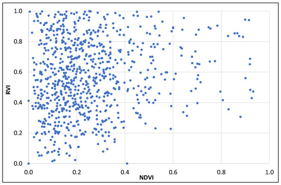
Figure 5.
Scatterplot of NDVI and RVI values over 1000 random points in the case study area.
In light of the above, monthly RVI and NDVI during the period from May 2019 to May 2020 were extracted from the Sentinel Hub service and interpreted. Monthly RVI results over the case study area are shown in Figure 6-left, while Figure 6-right shows the results of the NDVI (whereas a–l in both figures refers to months starting from May 2019). Higher RVI values that might correspond to vegetated areas are highlighted with a red colour in Figure 6-left, while the dark-green colour in Figure 6-right shows vegetation at the optical products. Examining Figure 6, it is evident that optical Sentinel-2 images (NDVI) can depict the phenological changes of the vegetation very well over the area of interest throughout the year. Indeed, during the summer period (June–August 2019), the NDVI is decreased compared to other periods.
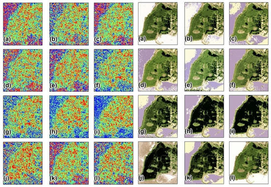
Figure 6.
Monthly Radar Vegetation Index—RVI—(left) and Normalized Difference Vegetation Index—NDVI—results (right) (a: May 2019, b: June 2019, c: July 2019, d: Aug. 2019, e: Sept. 2019, f: Oct. 2019, g: Nov. 2019, h: Dec. 2019, i: Jan. 2020, j: Feb. 2020, k: March 2020 and l: April 2020).
In contrast, the interpretation of the RVI is still problematic (Figure 6-left). However, some increase in vegetation (red colour) is evident during the months Dec. 2019 to Feb. 2020 (Figure 6-left, h–j). This increase of vegetation is also visible to optical products as well (Figure 6-right, h–j), indicating that a pattern over vegetated areas can be extracted from both Sentinel-1 and -2 sensors.
4.2. Estimating the Proportion of Vegetation Cover
Based on the RVI and NDVI, the proportion of vegetation cover was estimated using the Equations (3)–(6). The results from this application are shown in Figure 7. As mentioned earlier, the proportion of vegetation was estimated using two different models per vegetation index. Especially for the application of Equations (3) and (4), vegetated areas and non-vegetated areas need to be identified. The areas were selected using vector polygons from the OpenStreetMap service, and elsewhere (Google Earth environment). Green-colour polygons in Figure 7 show areas that were selected as “vegetated”, while yellow-colour polygons correspond to the “non-vegetated” areas. Figure 7a–c display the OpenStreetMap vegetated areas in the Google Earth environment, while Figure 7d–f show the non-vegetated areas. For estimating the proportion of vegetation cover from Equations (5) and (6), image image histogram statistics were used (max and min values). Based on the statistics, the RVI values for the vegetated and non-vegetated areas were 0.81 and 0.16, respectively, while the NDVI values for the vegetated and non-vegetated areas were estimated to be 0.80 and 0.27, respectively.
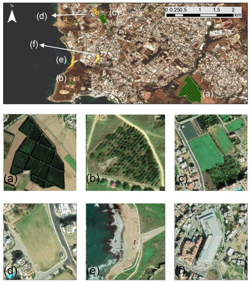
Figure 7.
Ground truth data as polygons extracted from the OpenStreetMap service used as “vegetated” and “non-vegetated” areas (top). (a–c) shows a high-resolution optical preview of the vegetated areas at Google Earth, while (d–f) the non-vegetated areas.
Figure 8a,b show the proportion of vegetation cover after the RVI (Equations (3) and (5) respectively), while Figure 8c,d show the results generated from the NDVI using Equation (4) and Equation (6), respectively. It is evident from Figure 8 that the proportion of vegetation per index using image statistics or OpenStreetMap data is quite similar. However, the results vary when we use optical and radar datasets. The general deviation of the results was expected, as we also saw this in the previous findings (Figure 4, Figure 5 and Figure 6). The RVI generates a noisier outcome (Figure 8a–b) compared to the results obtained from the NDVI (Figure 8c–d). Further elaboration of these results is discussed in the following section.
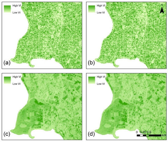
Figure 8.
The proportion of vegetation cover based on the RVI using Equation (3) (a) and Equation (5) (b), and the NDVI based on Equation (4) (c) and Equation (6) (d).
4.3. Evaluation of the Results
To compare the results, we firstly estimated the difference in the proportion of vegetation cover produced from the two different models. Figure 9a shows the difference the OpenStreetMap (Equation (3) and image statistics (Equation (5)) for the RVI, while Figure 9b shows the difference between the proportion of vegetation cover using the NDVI (Equations (4) and (6)). Higher differences between the two models are shown with a red colour while lower differences are estimated with a blue colour. However, examining the findings of Figure 9a,b, it is still difficult to compare the two outcomes. Differences in the pattern are apparent, indicating that the selection of the type of sensor (i.e., Sentinel-1, radar and Sentinel-2, optical sensors) influences the outcome.
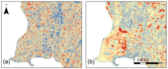
Figure 9.
(a) Difference of the proportion of vegetation cover as estimated from the Radar Vegetaton Index (RVI) based on Equations (3) and (5) and (b) Difference of the proportion of vegetation cover as estimated from the Normalized Difference Vegetation Index (NDVI) based on Equations (4) and (6). Higher difference values are indicated with red colour, while lower values with blue colour.
We further estimated the differences between the findings of Figure 9a,b. The results of this analysis are shown in Figure 10b. As shown in this Figure, differences in the estimation of the proportion of vegetation can vary significantly and over 40% using the optical (NDVI) and radar (RVI) indices. However, a closer look at these findings shows that the differences between these two types of satellite sources are minimal (< 10%) over vegetated areas (Figure 10c). This finding suggests that the estimation of the proportion of vegetation obtained by the Sentinel-1 and -2 sensors does not differ significantly over vegetated areas. This is also supported from the findings of Figure 6, whereas a similar pattern can be extracted for optical and radar products over vegetated areas (but not for other types of targets). Indeed, the use of the factor in Equation (2) can be adjusted for other types of targets. In addition, the scene classification product of the Sentinel-2 image of 13 May 2020 is shown in Figure 10d. Vegetated areas are shown in this Figure with a green colour, which recaps the findings of the results from Figure 10c, however with a lower resolution.
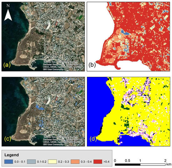
Figure 10.
(a) High-resolution satellite image over the case study area, (b) difference between the results of Figure 9a,b, (c) areas with minimum differences between the optical and the radar sensor indicated with blue colour over agricultural areas and (d) classification scene of Sentinel-2 images, whereas as vegetated areas are shown with green colour.
The results of Figure 10c were compared with a high-resolution optical satellite image available at the ArcGIS environment, at the northern part of the archaeological site of “Nea Paphos” (Figure 11a). Figure 11b shows a closer look at the findings of Figure 10c in this area, indicating that the difference is relatively low (blue colour in Figure 11b) over the vegetated areas. The results from the proportion of vegetation based on the optical Sentinel-2 sensor and using the NDVI and the OpenStreetMap inputs are shown in Figure 11c, while a high proportion of vegetation is highlighted with a yellow colour.
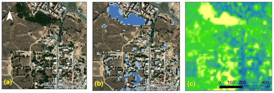
Figure 11.
(a) High-resolution satellite image over the case study area, (b) difference between the results of Figure 9a,b and (c) Normalized Difference Vegetation Index (NDVI)—proportion of vegetation.
While a direct comparison between the vegetation proportion from the RVI and the NDVI is not feasible, in an attempt to integrate the findings, we multiplied the RVI and the NDVI results (see Figure 8a–c), whereas high values will be expected in pixels with a high RVI and NDVI proportion of vegetation estimation, indicating vegetation presence. The results are shown in Figure 12. Figure 12a shows the multiplied RVI × NDVI results, whereas higher values indicated with a green colour highlight vegetated areas. Figure 12b–d is a focus of the red polygon of Figure 12a at the area of the historical Centre of Paphos (Figure 12b). Figure 12c is the proportion of vegetation as estimated from the NDVI using Equation (4), while Figure 12d is the multiplied RVI × NDVI. As shown, the latest image can better enhance the small differences in vegetation, also capturing some patterns from the buildings of the area.
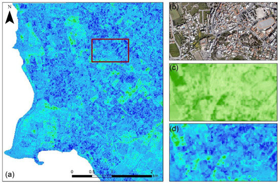
Figure 12.
(a) Multiplied Radar Vegetation Index (RVI) × Normalized Difference Vegetation Index (NDVI) result. Higher values indicating vegetated areas are shown with green colour (b) Red-Green-Blue (RGB) orthophoto of the red polygon of (a) showing the historical Centre of Paphos, (c) the NDVI—related proportion of vegetation and (d) the RVI × NDVI result.
5. Discussion
Overall, it was found that the use of optical and radar vegetation indices, namely the NDVI and the RVI, did not provide comparable results (see Figure 8). Optical indices were more eaily interpreted while the use of the RVI produced noisy data. However, some findings, such as the those of Figure 6, suggest that radar products can be used as an alternative to the optical data for detecting patterns (e.g., vegetation growth) in specific areas of interest.
To investigate the potential use of both proportions of vegetation indices derived from Sentinel-1 and -2 sensors, we multiplied the RVI × NDVI, as shown in Figure 12. This new product that integrates the RVI and NDVI outcomes can be used with the VV and VH polarizations of Sentinel-1 to create a new pseudo-colour composite. The unique characteristic of the radar sensors to depict urban areas (see also Figure 3c) can be used further to enhance the proportion of vegetation and urban areas. Such a new composite is shown in Figure 13. Using Sentinel-2 spectral bands 4 and 8, we can estimate the NDVI vegetation proportion while using the Sentinel-1 VV and VH polarizations; therefore, we can estimate the RVI vegetation proportion. The combination of the two new products generates the new RVI × NDVI vegetation proportion index, which can then be integrated again with the VV and the VH polarization to highlight vegetated areas (red colour under the “pseudo-colour composite of Figure 13) while buildings are also visible (with green colour in the same column).
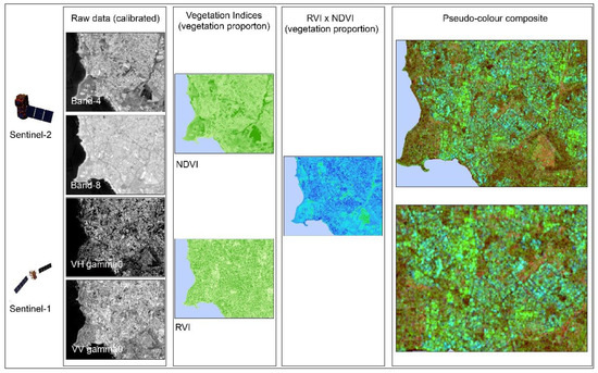
Figure 13.
New pseudo-colour composite on the right-left of the Figure integrating the RVI × NDVI vegetation proportion index, and the VV/VH polarizations from Sentinel-1. Vegetated areas are shown with red colour, while buildings with green colour. On the left side, the overall procedure (as explained in the previous sections) for estimating the RVI × NDVI index.
6. Conclusions
Estimating vegetation proportion through Earth Observation sensors is important, especially when dealing with the monitoring of hazards in the vicinity of archaeological sites. Vegetation cover is usually extracted from optical vegetation indices such as the NDVI. However, with the increasing availability of radar sensors like the Sentinel-1, radar-related vegetation indices have also been introduced in the literature.
The Sentinel Hub big data cloud platform can provide readily calibrated reflectance optical bands and VV/VH radar polarizations to end-users, and other ready products. Here, we explored the use of Sentinel-1 and -2 datasets for estimating vegetation proportion, as well as crowdsourced geo-datasets from the OpenStreetMap service, on an area in the western part of Cyprus
The overall findings indicate that Sentinel-1 and -2 indices can provide a similar pattern only over vegetated areas, which can be further elaborated to estimate temporal changes using integrated optical and radar Sentinel data. The use of the OpenStreetMap data was found very helpful as it allowed us to locate vegetated and non-vegetated areas with high accuracy, which would be difficult to achieve with the medium-resolution Sentinel data. Additionally, satellite images need to be radiometrically calibrated and corrected.
RVI and NDVI should be elaborated with caution since no direct correlation can be established. However, processed products such as differences of the vegetation proportion estimation can uncover similar patterns between the optical and the radar data. This allows us to fill gaps if no optical data are available. The combination of RVI × NDVI can enhance the presence of vegetated areas and can be integrated back to the VV and VH polarization (see Figure 13). The results from these findings can be further utilized so as to support the extraction of vegetation proportion using integrated radar and optical datasets, especially in areas with high cloud-coverage, supporting hazard analysis and risk management studies. In future, the author will explore ways to better adapt these two types of sensors for risk analysis at archaeological sites.
Funding
This article is submitted under the NAVIGATOR project. The project is being co-funded by the Republic of Cyprus and the Structural Funds of the European Union in Cyprus under the Research and Innovation Foundation grant agreement EXCELLENCE/0918/0052 (Copernicus Earth Observation Big Data for Cultural Heritage).
Acknowledgments
The author would like to acknowledge the “CUT Open Access Author Fund” for covering the open access publication fees of the paper. The author would like to acknowledge the use of the CORINE Land Cover 2018 (© European Union, Copernicus Land Monitoring Service 2018, European Environment Agency (EEA)”, in 2018: “© European Union, Copernicus Land Monitoring Service 2018, European Environment Agency (EEA)”), the Sentinel Hub (Modified Copernicus Sentinel data 2020/Sentinel Hub”), the OpenStreetMap service (© OpenStreetMap contributors) and Google Earth platform. Thanks, are also provided to the Eratosthenes Research Centre of the Cyprus University of Technology for its support. The Centre is currently being upgraded through the H2020 Teaming Excelsior project (www.excelsior2020.eu).
Conflicts of Interest
The author declares no conflict of interest
References
- Abate, N.; Lasaponara, R. Preventive archaeology based on open remote sensing data and tools: The cases of sant’arsenio (SA) and foggia (FG), Italy. Sustainability 2019, 11, 4145. [Google Scholar] [CrossRef]
- Garrote, J.; Díez-Herrero, A.; Escudero, C.; García, I. A framework proposal for regional-scale flood-risk assessment of cultural heritage sites and application to the castile and León region (central Spain). Water 2020, 12, 329. [Google Scholar] [CrossRef]
- Rodríguez-Navarro, P.; Gil Piqueras, T. Preservation strategies for southern morocco’s at-risk built heritage. Buildings 2018, 8, 16. [Google Scholar] [CrossRef]
- Tzouvaras, M.; Kouhartsiouk, D.; Agapiou, A.; Danezis, C.; Hadjimitsis, D.G. The use of sentinel-1 synthetic aperture radar (SAR) images and open-source software for cultural heritage: An example from paphos area in cyprus for mapping landscape changes after a 5.6 magnitude earthquake. Remote Sens. 2019, 11, 1766. [Google Scholar] [CrossRef]
- Nicu, C.I.; Asăndulesei, A. GIS-based evaluation of diagnostic areas in landslide susceptibility analysis of bahluieț river basin (moldavian plateau, NE Romania). Are neolithic sites in danger? Geomorphology 2018, 314, 27–41. [Google Scholar] [CrossRef]
- Luo, L.; Wang, X.; Guo, H.; Lasaponara, R.; Zong, X.; Masini, N.; Wang, G.; Shi, P.; Khatteli, H.; Chen, F.; et al. Airborne and spaceborne remote sensing for archaeological and cultural heritage applications: A review of the century (1907–2017). Remote Sens. Environ. 2019, 232, 111280. [Google Scholar] [CrossRef]
- Agapiou, A.; Lysandrou, V. Remote Sensing Archaeology: Tracking and mapping evolution in scientific literature from 1999–2015. J. Archaeol. Sci. Rep. 2015, 4, 192–200. [Google Scholar] [CrossRef]
- Tapete, D. Remote sensing and geosciences for archaeology. Geosciences 2018, 8, 41. [Google Scholar] [CrossRef]
- Traviglia, A.; Torsello, A. Landscape pattern detection in archaeological remote sensing. Geosciences 2017, 7, 128. [Google Scholar] [CrossRef]
- Rutishauser, S.; Erasmi, S.; Rosenbauer, R.; Buchbach, R. SARchaeology—Detecting palaeochannels based on high resolution radar data and their impact of changes in the settlement pattern in Cilicia (Turkey). Geosciences 2017, 7, 109. [Google Scholar] [CrossRef]
- Ghaffarian, S.; Rezaie Farhadabad, A.; Kerle, N. Post—Disaster recovery monitoring with google earth engine. Appl. Sci. 2020, 10, 4574. [Google Scholar] [CrossRef]
- Venkatappa, M.; Sasaki, N.; Shrestha, R.P.; Tripathi, N.K.; Ma, H.-O. Determination of vegetation thresholds for assessing land use and land use changes in cambodia using the google earth engine cloud-computing platform. Remote Sens. 2019, 11, 1514. [Google Scholar] [CrossRef]
- Abate, N.; Elfadaly, A.; Masini, N.; Lasaponara, R. Multitemporal 2016–2018 sentinel-2 data enhancement for landscape archaeology: The case study of the foggia province, southern Italy. Remote Sens. 2020, 12, 1309. [Google Scholar] [CrossRef]
- European Copernicus Programme. Available online: https://www.copernicus.eu/en (accessed on 14 June 2020).
- Sentinel Hub. Available online: https://www.sentinel-hub.com (accessed on 14 June 2020).
- Dana Negula, I.; Moise, C.; Lazăr, A.M.; Rișcuța, N.C.; Cristescu, C.; Dedulescu, A.L.; Mihalache, C.E.; Badea, A. Satellite remote sensing for the analysis of the micia and germisara archaeological sites. Remote Sens. 2020, 12, 2003. [Google Scholar] [CrossRef]
- Lin, S.-K. Satellite Remote Sensing: A New Tool for Archaelogy; Lasaponara, R., Masini, N., Eds.; Springer: Berlin/Heidelberg, Germany, 2012; Volume 4, pp. 3055–3057. ISBN 978-90-481-8800. [Google Scholar]
- Roy, A.; Inamdar, B.A. Multi-temporal land use land cover (LULC) change analysis of a dry semi-arid river basin in western India following a robust multi-sensor satellite image calibration strategy. Heliyon 2019, 5, e01478. [Google Scholar] [CrossRef] [PubMed]
- Haque, I.; Basak, R. Land cover change detection using GIS and remote sensing techniques: A spatio-temporal study on Tanguar Haor, Sunamganj, Bangladesh. Egypt. J. Remote Sens. Sp. Sci. 2017, 20, 251–263. [Google Scholar] [CrossRef]
- Abd El-Kawy, O.R.; Rød, J.K.; Ismail, H.A.; Suliman, A.S. Land use and land cover change detection in the western nile delta of Egypt using remote sensing data. Appl. Geogr. 2011, 31, 483–494. [Google Scholar] [CrossRef]
- Hegazy, I.R.; Kaloop, M.R. Monitoring urban growth and land use change detection with GIS and remote sensing techniques in daqahlia governorate Egypt. Int. J. Sustain. Built Environ. 2014, 4, 117–124. [Google Scholar] [CrossRef]
- Alijani, Z.; Hosseinali, F.; Biswas, A. Spatio-temporal evolution of agricultural land use change drivers: A case study from Chalous region, Iran. J. Environ. Manag. 2020, 262, 110326. [Google Scholar] [CrossRef]
- Chyla, J.M. How can remote sensing help in detecting the threats to archaeological sites in upper Egypt? Geosciences 2017, 7, 97. [Google Scholar] [CrossRef]
- Xu, Y.; Yu, L.; Zhao, Y.; Feng, D.; Cheng, Y.; Cai, X.; Gong, P. Monitoring cropland changes along the Nile River in Egypt over past three decades (1984–2015) using remote sensing. Int. J. Remote Sens. 2017, 38, 4459–4480. [Google Scholar] [CrossRef]
- Senanayake, S.; Pradhan, B.; Huete, A.; Brennan, J. Assessing soil erosion hazards using land-use change and landslide frequency ratio method: A case study of sabaragamuwa province, Sri Lanka. Remote Sens. 2020, 12, 1483. [Google Scholar] [CrossRef]
- Viana-Soto, A.; Aguado, I.; Salas, J.; García, M. Identifying post-fire recovery trajectories and driving factors using landsat time series in fire-prone mediterranean pine forests. Remote Sens. 2020, 12, 1499. [Google Scholar] [CrossRef]
- Howland, D.M.; Ian Jones, W.N.I.; Najjar, M.; Levy, E.T. Quantifying the effects of erosion on archaeological sites with low-altitude aerial photography, structure from motion, and GIS: A case study from southern Jordan. J. Archaeol. Sci. 2018, 90, 62–70. [Google Scholar] [CrossRef]
- Burry, L.B.; Palacio, I.P.; Somoza, M.; Trivi de Mandri, E.M.; Lindskoug, B.H.; Marconetto, B.M.; D’Antoni, L.H. Dynamics of fire, precipitation, vegetation and NDVI in dry forest environments in NW Argentina. contributions to environmental archaeology. J. Archaeol. Sci. Rep. 2018, 18, 747–757. [Google Scholar] [CrossRef]
- Department of Antiquities. Archaeological Sites. Available online: http://www.mcw.gov.cy/mcw/da/da.nsf/DMLsites_en/DMLsites_en?OpenDocument (accessed on 14 June 2020).
- CORINE 2018 Program. Available online: https://land.copernicus.eu/pan-european/corine-land-cover (accessed on 14 June 2020).
- Cuca, B.; Agapiou, A. Impact of land use change to the soil erosion estimation for cultural landscapes: Case study of Paphos district in Cyprus. In The International Archives of the Photogrammetry, Remote Sensing and Spatial Information Sciences; Spatial Inf. Sci., XLII-5/W1; 2017; pp. 25–29. Available online: https://doi.org/10.5194/isprs-archives-XLII-5-W1-25-2017 (accessed on 9 July 2020).
- Agapiou, A.; Alexakis, D.D.; Lysandrou, V.; Sarris, A.; Cuca, B.; Themistocleous, K.; Hadjimitsis, D.G. Impact of urban sprawl to archaeological research: The case study of Paphos area in Cyprus. J. Cult. Herit. 2015, 16, 671–680. [Google Scholar] [CrossRef]
- Agapiou, A.; Lysandrou, V.; Alexakis, D.D.; Themistocleous, K.; Cuca, B.; Sarris, A.; Argyrou, N.; Hadjimitsis, D.G. Cultural heritage management and monitoring using remote sensing data and GIS: The case study of Paphos area, Cyprus. CEUS Comput. Environ. Urban Syst. 2015, 54, 230–239. [Google Scholar] [CrossRef]
- Panagos, P.; Borrelli, P.; Poesen, J.; Ballabio, C.; Lugato, E.; Meusburger, K.; Montanarella, L.; Alewell, C. The new assessment of soil loss by water erosion in Europe. Environ. Sci. Policy 2015, 54, 438–447. [Google Scholar] [CrossRef]
- OpenStreetMap Service. Available online: https://www.openstreetmap.org/ (accessed on 14 June 2020).
- Schultz, M.; Voss, J.; Auer, M.; Carter, S.; Zipf, A. Open land cover from OpenStreetMap and remote sensing. Int. J. Appl. Earth Obs. Geoinf. 2017, 63, 206–213. [Google Scholar] [CrossRef]
- Zhao, W.; Bo, Y.; Chen, J.; Tiede, D.; Blaschke, T.; Emery, J.W. Exploring semantic elements for urban scene recognition: Deep integration of high-resolution imagery and OpenStreetMap (OSM). ISPRS J. Photogramm. Remote Sens. 2019, 151, 237–250. [Google Scholar] [CrossRef]
- Johnson, A.B.; Iizuka, K.; Bragais, A.M.; Endo, I.; Magcale-Macandog, B.D. Employing crowdsourced geographic data and multi-temporal/multi-sensor satellite imagery to monitor land cover change: A case study in an urbanizing region of the Philippines. Comput. Environ. Urban Syst. 2017, 64, 184–193. [Google Scholar] [CrossRef]
- Sentinel-ub Services, Custom Scripts. Available online: https://custom-scripts.sentinel-hub.com/sentinel-1/radar_vegetation_index (accessed on 8 June 2020).
- QGIS. A Free and Open Source Geographic Information System. Available online: https://www.qgis.org/en/site/ (accessed on 2 July 2020).
© 2020 by the author. Licensee MDPI, Basel, Switzerland. This article is an open access article distributed under the terms and conditions of the Creative Commons Attribution (CC BY) license (http://creativecommons.org/licenses/by/4.0/).