Multi-Pose Face Recognition Based on Deep Learning in Unconstrained Scene

Abstract

At present, deep learning drives the rapid development of face recognition. However, in the unconstrained scenario, the change of facial posture has a great impact on face recognition. Moreover, the current model still has some shortcomings in accuracy and robustness. The existing research has formulated two methods to solve the above problems. One method is to model and train each pose separately. Then, a fusion decision will be made. The other method is to make “frontal” faces on the image or feature level and transform them into “frontal” face recognition. Based on the second idea, we propose a profile to the frontal revise mapping (PTFRM) module. This module realizes the revision of arbitrary poses on the feature level and transforms the multi-pose features into an approximate frontal representation to enhance the recognition ability of the existing recognition models. Finally, we evaluate the PTFRM on unconstrained face validation benchmark datasets such as Labeled Faces in the Wild (LFW), Celebrities in Frontal Profile (CFP), and IARPA Janus Benchmark A(IJB-A). Results show that the chosen method for this study achieves good performance.

1. Introduction

In recent years, the emergence of deep learning has achieved great success in the field of face recognition. However, in unconstrained scenes, factors such as changes in the illumination, occlusion, pose, and expression still largely interfere with the accuracy and robustness of face recognition. The current models have some deficiencies in accuracy and robustness, especially with large angles and pose variations. Intuitively, the main reason is that the number of the front faces and multi-pose faces in the training set are highly unbalanced because detecting multi-pose faces is more difficult than finding front faces. In addition, given the pose variations, learning the feature representation with geometric invariance to large pose variations directly is challenging.

Existing face recognition methods based on deep learning mainly include the following modules: image preprocessing, training a convolutional neural network (CNN) to extract features, face verification, and recognition. Image preprocessing includes face detection, alignment, normalization, and random flipping. It unifies the facial image into a fixed size as the input of the CNN network. The target of face verification and recognition is achieved by comparing the voting score obtained by the similarity measure or the Euclidean distance measure with the threshold.

In this study, we propose a profile to the frontal revise mapping (PTFRM) module based on Residual Nets(ResNet). On the one hand, we use a branch of pose estimation when an image is input, as shown in Figure 1. The input image and its corresponding key points (center of the left eye, center of the right eye, nose tip, left mouth corner, and right mouth corner) are computed by this branch to obtain a pose estimation that includes the three components of pitch, yaw, and roll [1]. The pose labels of each face image are obtained by the pose mapping function. On the other hand, we add the PTFRM module branch into CNN. The PTFRM module consists of our transformation layer (defined in the paper), fully connected layer, and batchnormal layer. The transformation layer takes the features of the previous layer and the pose classes of the new branch as input. Then, it selects the transformation vector with the pose classes to realize the revision of the arbitrary pose features. After the transformation layer, we add the full connection layer and the batchnormal layer to output a new feature, which is the representation of the approximate frontal feature space. The PTFRM module realizes the transformation from the multi-pose space to the approximate frontal feature space.

As shown in Figure 1, according to the pose categories obtained by the pose module and the basic features obtained by the shared CNN, we transform the basic features, which imply different attitude information, into approximate frontier features. We also use pose loss and softmax loss to constrain the optimization of network parameters.

The main contributions of this study are as follows:

• The PTFRM module is proposed to complete feature transformation based on CNN and transform the features of different poses linearly into the frontal features. It improves the computational efficiency and achieves outstanding recognition accuracy in three datasets of LFW, CFP, and IJB-A.
• The pose category is estimated by combining the pitch, yaw, and roll, which fully considers the generalization ability of the model to perform face recognition under different poses. Therefore, the entire model is called PTFRM_PYR.
• The pose loss is adopted, and the pose category label is used to optimize the conversion from the multi-pose space to the approximate frontal feature space and to enhance the recognition ability and robustness of the model for multiple poses.

2. Related Works

From DeepID 1 [2] proposed by Sun in 2014 to InsightFace [3,4] proposed by Deng in 2019, deep learning has rapidly been developed in face recognition applications and has become the mainstream method for face recognition. The existing research based on CNN adopts different loss functions for optimization, such as softmax loss [5], center loss [6], triplet loss [7], arcloss [4], and RegularFace loss [8]. Among them, center loss reduces the intraclass distance and enhances the recognition ability, while strengthening the interclass distance and enhancing the classification and recognition ability, which is representative in the loss functions.

For unconstrained scenes, especially for large angle and multi-pose face recognition, the current solutions are as follows. The first solution is to model each pose separately, and then discriminate the outcome by merging the results of each pose assessment, such as Pose-Aware Models(PAMs) [9]. The PAMs classify the face images according to the yaw angle. They construct a network to extract features for each type of face image. They fuse all the features to construct a new feature representation for face recognition. However, modeling each pose separately greatly consumes computing resources and time resources.

The second solution is to change a side face to a frontal face at the image level, which contains many excellent results. Hayat, M et al. [10] used a spatial transformer network to approximate the frontal view of a non-frontal image. Stacked Progressive Auto-Encoders(SPAE) [11] progressively maps the face images at large poses to a virtual view at smaller ones through a stack of several autoencoders. Yin et al. [12] incorporated a 3D morphable face model into the Generative Adversarial Networks(GAN) structure to guide the generator to create a frontal face. In Disentangled Representation learning-Generative Adversarial Network (DR-GAN) [13,14], the decoder synthesizes a face at a specified pose using identity representation and a pose label. Face Normalization Model(FNM) [15] can recover a canonical-view and expression-free image and directly improve the performance of the face recognition model by generating a confrontation network. These methods regenerate the face image with the pose into a frontal face image. Then, face recognition is performed according to the existing face recognition methods. Nonetheless, the process of regenerating an image is complicated and time-consuming. Causing distortion and increasing the difficulty of recognition is easy in the process of regenerating a new image.

The third solution is to change the poses to create a frontal image at the feature level and to revise the multi-pose feature to improve the ability of face recognition. Template Deep Reconstruction Model(TDRM) [16] uses a sparse representation-based method for pose approximation. The Deep Residual Equivariant Mapping(DREAM) model proposed by Rong et al., [17] maps profile features to the frontal features. The DREAM model only considers the yaw pose component, which is not comprehensive.

The PTFRM module that we propose considers not only the yaw component but also the pitch and roll components. It makes full use of the pose information of the face to obtain the corresponding pose class label. We can directly obtain the pose tags for large-angle and multi-pose face images, which makes up for the shortcomings of the DREAM model. We also use pose loss to optimize the feature transformation from the multi-pose feature space to approximate a frontal space, thus enhancing the generalization ability of the model and strengthening the recognition ability for multi-pose features.

3. PTFRM Module

Figure 2 shows the principle of the proposed method. The feature extraction network takes the face images with various poses as inputs and extracts the original feature representation, which is mapped into the approximate frontal feature space by the PTFRM module. With only one feature extraction network and a PTFRM module added at the end of the network, we can achieve a “frontal” pose at the feature level, which greatly saves space and time resources. This approach maintains end-to-end characteristics and makes the entire process easy to train and verify.

3.1. Pose Estimation and Classification

We assume that facial landmark is detected. We take Face Image I and estimate five key points, which include the center of the left eye and the right eye, the nose tip, the left mouth, and the right mouth.

Pose estimation is used to estimate the angle values of the three pose components (pitch, yaw, and roll), given a two-dimensional face image. This study also uses the Perspective-n-Point (PnP) method [1] to realize pose estimation. This method makes the 2D projection of 3D feature points on the model coincide with the feature points on the 2D face image as much as possible by rotating the default 3D mode. The rotation angle of the 3D model is the required three-pose angles.

We can obtain the three pose components, namely, pitch, yaw, and roll, from the pose estimation. The three pose components are further processed so that the information they contain can be used. According to Part I, most models only consider the yaw component. More scientifically, the influence of the three pose components should be equally weighted. Our main objective is to combine the three pose components and classify the poses to transform the features of multi-pose faces to the front feature space. Given that the poses with different classifications have different degrees of correction, the classification formula is as follows:

$$\mathrm{N}\left(p,y,r\right)=\{\begin{array}{ll}0,& \left(p+y+r\right)\le 25\\ 1,& 25<\left(p+y+r\right)\le 45\\ 2,& 45<\left(p+y+r\right)\le 75\\ 3,& 75<\left(p+y+r\right)\le 90\\ 4,& \left(p+y+r\right)>90\end{array}$$

(1)

where $p$ represents the pose component pitch, $y$ represents the yaw, $r$ represents the roll, and 0, 1, 2, 3, 4 indicate the classification labels for different poses; 25, 45, 75, 90 are the default hyperparameters, which serves as the threshold to classify pose categories. As a rule of thumb, each component should be less than 10 in the case of small positive or pose changes, and less than 30 in the case of large pose changes. Therefore, we roughly divided poses into several different levels according to the sum of the three pose components, i.e., the deviation from the fully frontal angle. Different mapping relationships are used to provide a mathematical basis for the realization of the different degrees of revision.

3.2. PTFRM Module

The PTFRM module consists of a custom transformation layer, a fully connected layer, and a batchnormal layer. The transformation layer takes the feature of the CNN and the corresponding pose class as input controls the projection matrix according to the pose class and maps the original feature representation to the new feature representation. Our essential objective is to map the features of the multi-pose angle feature space to the approximate frontal feature space through the transformation layer, which is a transformation at the feature level. Compared with the transformation at the image level, our proposed idea is more efficient and concise.

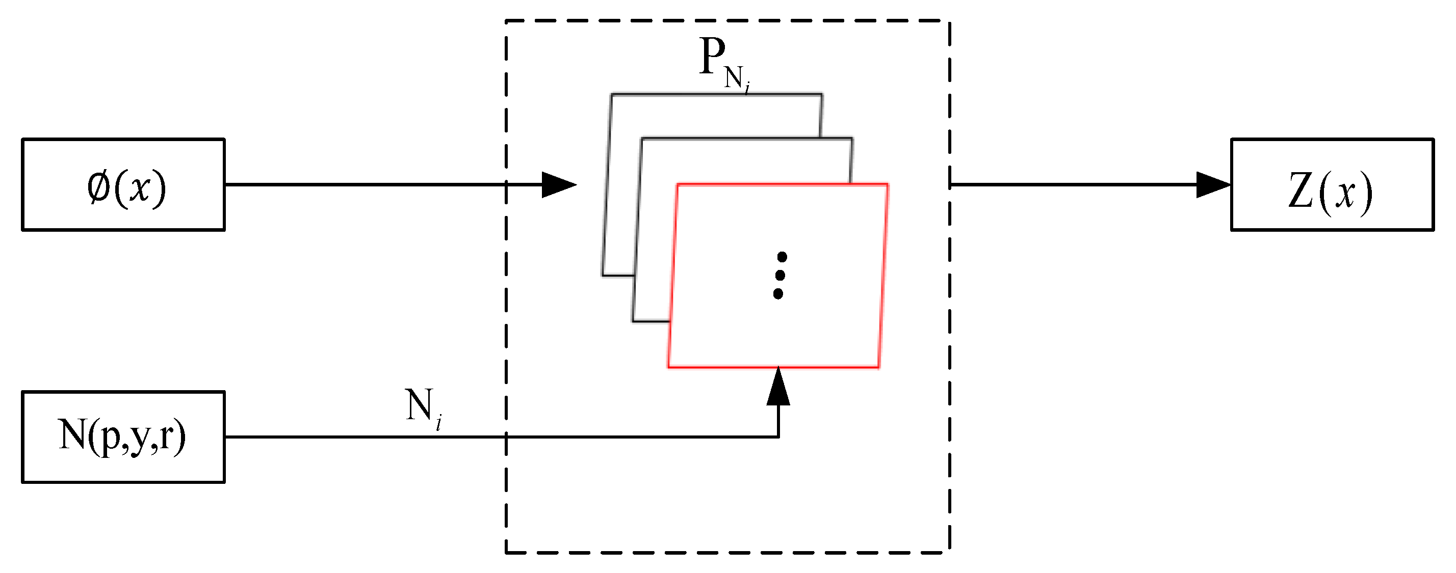
Figure 3 shows the transformation process of the transformation layer. $x$ represents the face image input. The output of the feed-forward CNN is $\varphi \left(x\right)$, which is a basic feature representation. $N_i$ is the corresponding pose class of the face image, which is obtained from the pose estimation and classification function $N\left(p,y,r\right)$. New feature representation $Z\left(x\right)$ is obtained through the transformation layer. The mathematical expression is as follows:

$$Z\left(x\right)=P_{N_i}\varphi \left(x\right)$$

(2)

where $P_{N_i}$ is the projection matrix corresponding to the pose class $N_i$, which represents the pose class corresponding to the input $x$. $Z\left(x\right)$ represents the transformed feature representation of $\varphi \left(x\right)$. Then we obtain the output feature representation of the PTFRM module through the fully connected layer and batchnormal layer. This representation is also the feature representation extracted in the validation stage of this study.

3.3. Optimizing Objectives

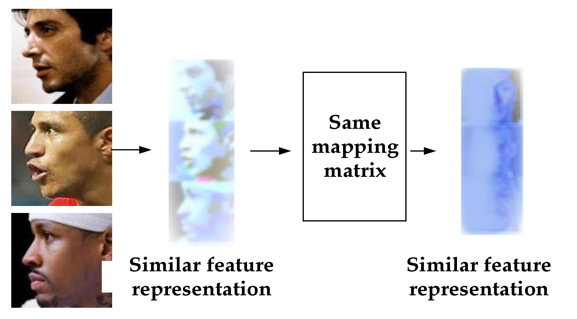
From Section 2, we can see that the mapping function in the study does not specifically address the true identity of the face. Only the face image is classified. As long as the face with the same pose class does not need its identity tag, the same mapping relationship maps the basic feature to approximate frontal feature representation. For faces with the same identity, the PTFRM module uniformly converts the face features of different poses into approximately positive features. This process narrows the distance within the class. However, for faces with similar facial features, the same posture, and different categories, the new feature representation is still similar after the mapping process of the PTFRM module. Therefore, in the optimization process, the existence of small differences among different categories must be considered, as shown in Figure 4:

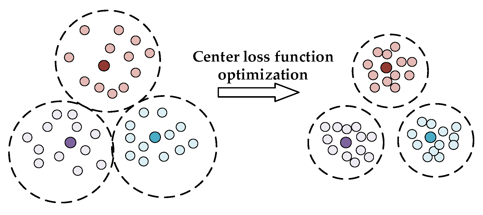
To solve the problem of the distance among classes being too small, we consider using identity tags as constraints. After the mapping module outputs the features, we construct a feature center for the features of the same identity class. The feature center is a standard feature representation of the frontal face image of the same person. Next, we construct an optimization function to minimize the distance between feature representations and the feature center of all the same identities. Thus, all similar feature representations are centered on feature centers and the cohesion between the features is enhanced. Then, we can reduce the intraclass distance and enhance the interclass distance. We define the target loss function as follows:

$$L_p=\frac{1}{2}{{\displaystyle \sum }}_{1=i}^m\Vert Z\left(x_i\right)-f_s^{yi}{\Vert }_2^2$$

(3)

where $L_p$ is the center loss function, $m$ represents the number of samples of a batch, and $x_i$ is the $i\text{-}th$ sample. $Z\left(x_i\right)$ is the map-converted feature representation, and $f_s^{y_i}$ is the feature center of the identity class, which is also a feature representation.

Figure 5 shows the function diagram.

The deep color point is the feature center, and the same color is the same category. By constructing a feature center and constraining distance, similar features can be compact, and the inter-class distance increases, which is conducive to target classification.

$f_s^{y_i}$ cannot be directly obtained. Thus, we update the center in each batch, that is, we randomly initialize the center, and calculate the distance between the current data and the center in each batch. Then, we add the distance in the gradient form to the center. The optimization formula is as follows:

$$∆f_s^j=\frac{{{\displaystyle \sum }}_{i=1}^m\delta \left(y_i=j\right)\times \left(f_s^{y_i}-Z\left(x_i\right)\right)}{1+{{\displaystyle \sum }}_{i=1}^m\delta \left(y_i=j\right)}$$

(4)

where $j$ represents the $j\text{-}th$ feature center, and $m$ represents the size of the mini-batch. $\delta \left(y_i=j\right)$ represents where each sample only affects the corresponding feature center.

Supposing that the loss function of the classification task is $L_c$, the formula is as follows:

$$L_c=-\frac{1}{m}{{\displaystyle \sum }}_{i=0}^m\log \frac{e^{{\theta }_{y_i}^T{x}_i+b_i}}{{{\displaystyle \sum }}_{j=1}^n{e}^{{\theta }_j^T{x}_i+b_i}}$$

(5)

where $m$ is the number of samples in a batch. ${\theta }_{y_i}^T$ is the weight vector corresponding to the category $y_i$ and the $i\text{-}th$ sample. $b_i$ is the offset value used for the $i\text{-}th$ sample. $n$ is the number of identity classes.

Given that we have to learn two interrelated tasks, we use the same training set. We consider using the multi-task joint supervision learning method. Then, we set the final loss function to $L_{loss}$, which is defined as follows:

$$L_{loss}=\lambda L_p+L_c$$

(6)

where $\lambda$ is a hyperparameter, which is mainly used to balance the convergence of a network. If $\lambda$ is too large, the network will be over-fitting. If $\lambda$ is too small, it will have difficulty being convergent. In this study, this hyperparameter is set to 0.005.

4. Experiments

The effective training of the deep face recognition model is based on a sufficiently large training dataset. We choose the CASIA-Webface [18] dataset as the training set. After cleaning, the amount of data is approximately 1 M with more than 10,000 categories. We firstly perform accurate face detection through the Multitask Cascaded Convolutional Networks(MTCNN) [19] model and obtain the coordinates of the five key points corresponding to the face image. The affine transformation between the key points is used to align the faces to obtain the inputs of the CNN. Then we normalize each image size to 112 × 112. At the same time, we use the estimation of the coordinates of the five points to obtain the pose results. Then, we obtain the pose categories through the pose classification function $N\left(p,y,r\right)$.

After using the PnP method mentioned in Section 3.1 to solve the initial solution, a deep CNN, which adopts the Visual Geometry Group(VGG) [20] network architecture, is used to learn a direct mapping from the picture to the three pose angles. The pose estimation network is trained separately within the images and the initial solution calculated by the PnP. This network does not participate in iterations during trunk training.

The backbone model we adopt is based on LResnet50E-IR [3,4] in ArcFace, which is used to find the segmentation hyperplane of the feature space. However, it is no longer based on the segmentation of the Euclidean feature distance space. Instead, it is only mapped to the cosine angle space to find the appropriate segmentation hyperplane. The model can achieve efficient and robust segmentation in the angle space, while the angle space-based metrics closely matches with the cosine similarity-based verification.

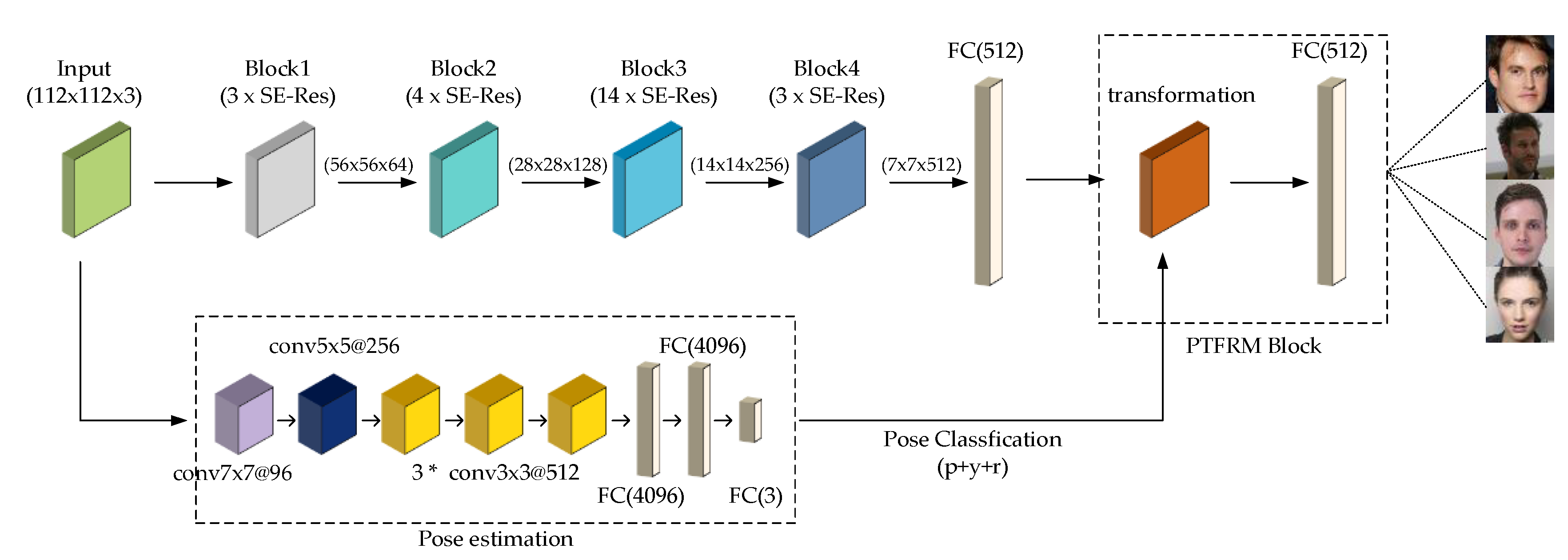
The overall network structure is shown in Figure 6.

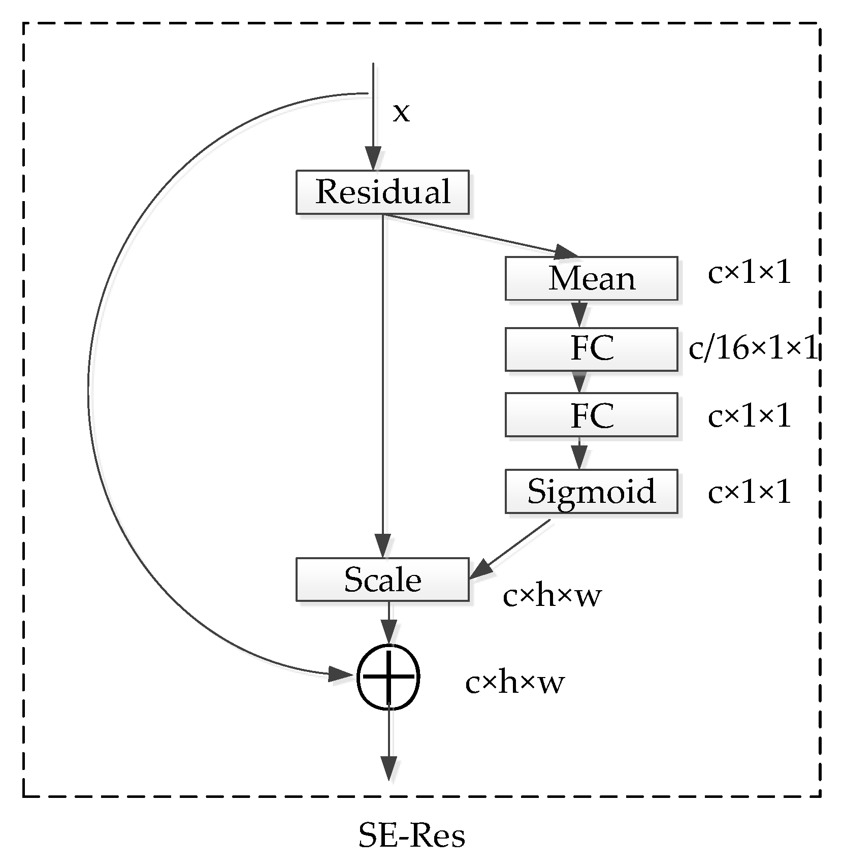
The network starts with an input layer. Then, it gradually extracts features from coarse to fine through four blocks, and the size of the output feature graph of each block is halved. Block1 contains 3 Squeeze-and-Excitation residual (SE-Res) blocks and the output feature channel is 64. Block2 contains 4 SE-Res blocks and the output feature channel is 128. Block3 contains 14 SE-Res blocks and the output feature channel is 256. Block4 contains 3 SE-Res blocks and the output feature channel is 512. If the input image size is 112 × 112, the feature sizes of the blocks are 56 × 56, 28 × 28, 14 × 14, and 7 × 7, respectively. Finally, a dropout layer is used to prevent overfitting, and the 512-dimensional feature representation is output through the full connection layer. After each full convolutional layer, the BN layer is used to accelerate network convergence and the PReLU function is used to enhance nonlinear mapping capability. The structure of SE-Res [21] is shown in Figure 7.

Based on the Res structure, SE-Res uses the dependency relationship between feature channels to learn the weight coefficient of each feature map to represent the important relationship of the feature map. Then, the feature map of the Res block is multiplied channel by channel to obtain the feature map representation containing a lot of information. SE-Res can suppress unimportant features and amplify important features.

In this study, we chose CASIA-Webface dataset as the training set, while the LFW, CFP, and IJB-A dataset are only used for evaluating algorithm performance, they do not actually participate in the updating of the network parameter $W$.

We adopt joint training and trained pose loss and softmax loss on the same dataset at the same time. Then, we set the weight of the pose loss to 0.005. The initial learning rate is 0.005 and the batch size is 32.

4.1. Validation on LFW Dataset

The Labeled Faces in the Wild (LFW) dataset is one of the main test sets for studying face recognition in unconstrained scenarios. Its images are derived from the images in movies, including face images of various scenes. The LFW dataset contains more than 13000 face images, with approximately 1680 categories [22]. Moreover, it is used for face verification. The test protocol diagram is as Figure 8.

4.1.1. Ten-Fold Cross-Validation

The standard LFW evaluation protocol defines a verification experiment under ten-fold cross-validation with 300 genuine comparisons and 300 impostor comparisons per fold. Through the feature extraction network designed in Figure 6, we obtain 512 dimensions that correspond with output feature pairs. Each pair of feature representations receives a corresponding similarity score by calculating a distance. Furthermore, we classify all distances by choosing appropriate thresholds. Finally, we compare the actual classification to acquire the final accuracy on the test set. Using a direct calculation of the distance, we perform ten-fold cross-validation. We take turns to use 9 folders for training, these folders are used to determine the optimal value of hyperparameter threshold. In the last folder, we use the best threshold to achieve accuracy and use the average of the results for 10 times to estimate the algorithm accuracy. Figure 9 shows the feature distances and labels of 6000 image pairs. We can set a threshold. If the distance of the image pairs is smaller than the threshold, the image pairs will be set to the same category. If the distance of the image pairs is larger than the threshold, the image pairs will be set to different categories. Then, we can calculate the accuracy. Evidently, the maximum accuracy is achieved when the threshold value is around 1.5.

From

Table 1. Accuracy of related algorithms on the LFW test set.

Algorithms	LFW (Accuracy ± Std)
DeepFace [23]	95.92% ± 0.29%
COTS matcher [24]	98.2% ± 0.6%
DeepID-2+ [25]	98.70% ± 0.15%
Chen et al. [26]	99.16% ± 0.31%
PTFRM_PYR	99.43% ± 0.16%

, we can see that the average accuracy of the algorithm in this study is 99.43%, and the deviation is ±0.16%, which is better than the comparison algorithm. The results show that the network of the algorithm in this study is very stable and has a strong generalization ability. The advantage of this algorithm is mainly attributed to the stable basic network, which can steadily extract the basic features with strong expression ability. However, the PTFRM module has good transformation mapping ability under the optimization of pose loss, which can transform the feature of the multi-pose into a front feature and enhance the discrimination of those misclassified features.

4.1.2. Shuffle-Split Cross-Validation

Although ten-fold cross-validation is the standard validation method of the LFW dataset, we use shuffle-split cross-validation to explore the influence of different proportions of training sets on the performance of the validation algorithm.

During the validation of LFW, 6000 pairs are used for face verification, 3000 pairs of which belong to the same tags, and 3000 pairs of which belong to the different target tags. We divided the dataset into the training set and the test set after random shuffling, and the proportion of training set gradually increased from 0.1 to 0.9. There are 9 groups of experiments. We repeated the experiment 10 times in each group and then used the average and median of the results to estimate the accuracy of the algorithm.

Table 2. Accuracy of different validation methods on the LFW test set.

Training Set Proportion	0.1	0.2	0.3	0.4	0.5	0.6	0.7	0.8	0.9
Average accuracy	99.29%	99.32%	99.36%	99.36%	99.35%	99.39%	99.41%	99.43%	99.43%
Median accuracy	99.35%	99.34%	99.38%	99.36%	99.33%	99.40%	99.39%	99.42%	99.42%
Standard deviation	0.16%	0.09%	0.05%	0.08%	0.08%	0.13%	0.14%	0.14%	0.20%

shows the results.

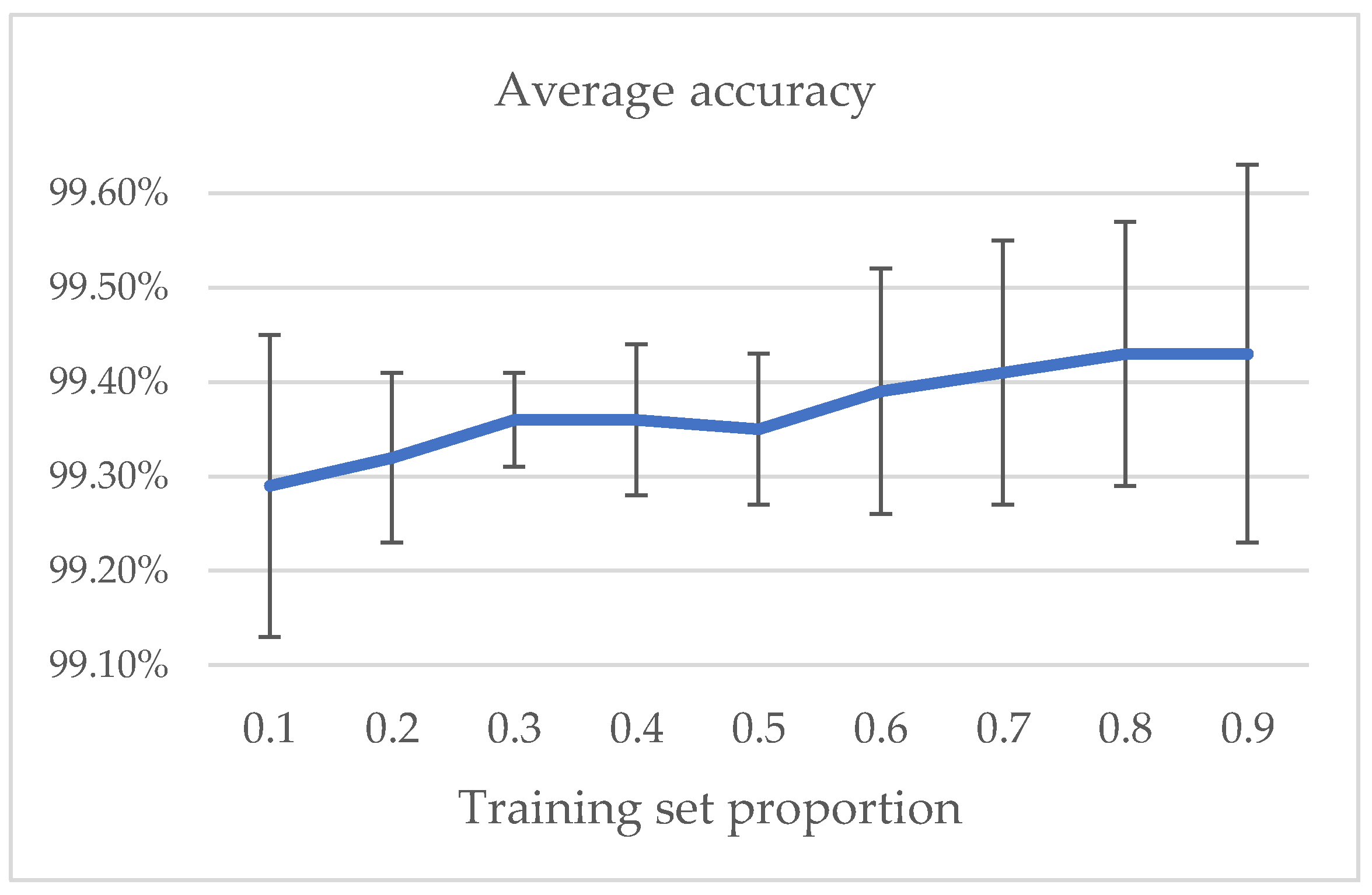
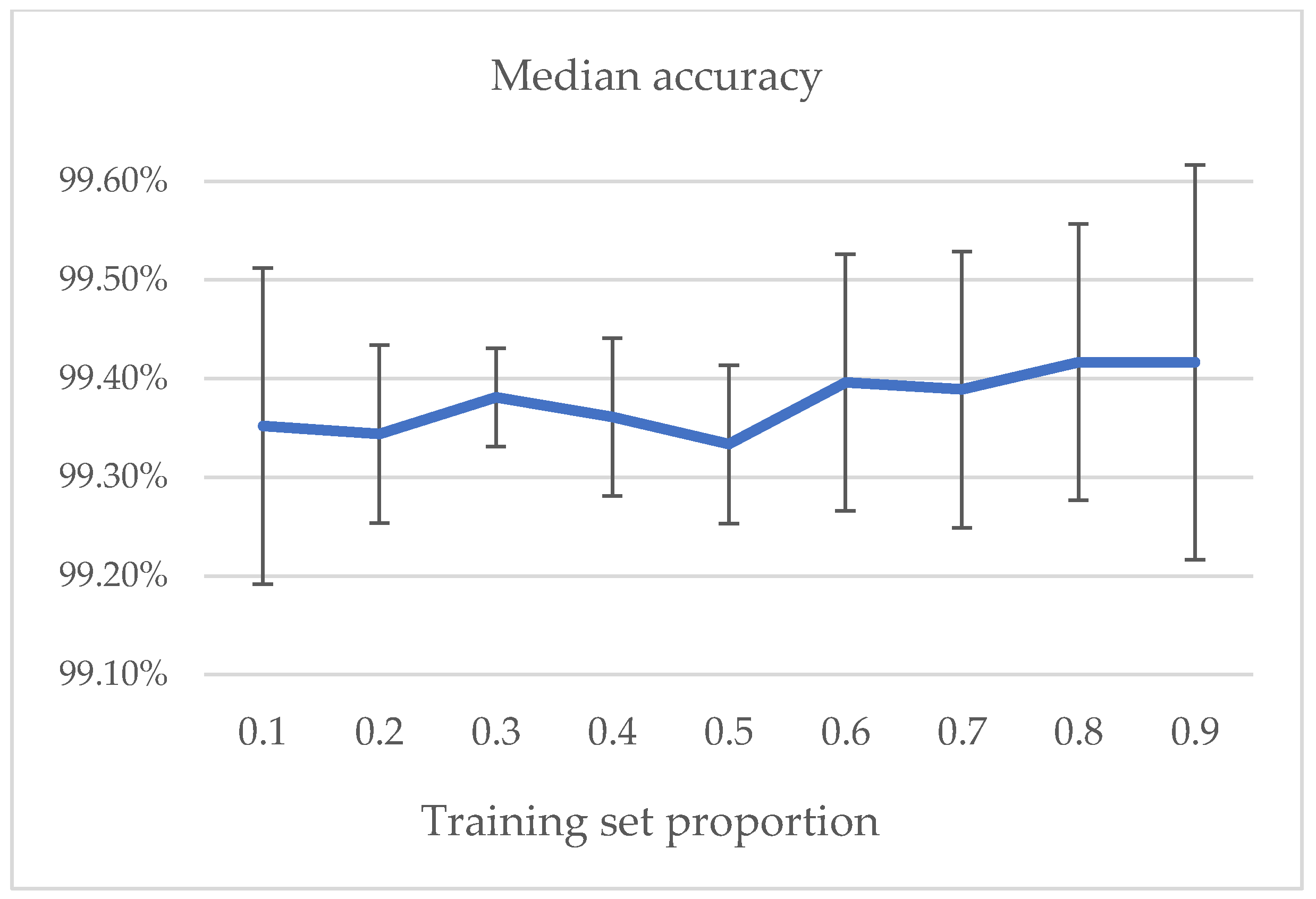
As shown in Figure 10 and Figure 11, as the proportion of training set increases, the average and median accuracy rise, but the overall change range is not large, which shows good algorithm performance. A small training set can also have good performance, which indicates that the model has great stability. From the perspective of standard deviation, when the training dataset is small, the stability of the model obtained is relatively poor, and the standard deviation is relatively large. In the process of increasing the training dataset, sufficient training data are selected to obtain a stable model. However, as test samples reduce, a few wrong judgments have great impact on the standard deviation of the accuracy. That is the reason the standard deviation goes up after group 6.

Therefore, we draw the following conclusions:

• The higher the proportion of the training data, the higher the accuracy of model verification.
• In small datasets, a few test samples will increase the standard deviation of accuracy.
• For the LFW dataset, the ten-fold cross-validation is a good way to estimate generalization performance, but the more appropriate proportion of the training dataset is maybe 0.3–0.8.

4.2. Validation on CFP Dataset

As a common face dataset, the Celebrities in Frontal Profile (CFP) dataset focuses on the profile faces. It contains a total of 500 face images of individuals. The face image set of each person contains 10 frontal face images, 4 side face images, and a total of 7000 images in the dataset [27]. The CFP dataset is used for testing face verification. The test protocol is similar to the LFW dataset, but the CFP dataset has two types of test methods. The first is the frontal-frontal (ff) mode, in which we select verification pairs from the frontal face images. The other is the frontal-profile (fp) mode, in which one of the validated images is selected from the frontal faces and the other from the side faces. This test protocol is equivalent to separating the unified test of the LFW dataset into two types. One type verifies the ability of the algorithm to distinguish frontal faces, and the other verifies the ability to distinguish the side faces. Figure 12 and Figure 13 show the schematic diagram of the CFP test protocol.

The test methods of the ff-mode and the fp-mode are the same as the LFW dataset. We obtain the feature representation through the network, calculate the distance between the features, and obtain the classification through a unified threshold. Finally, we achieve accuracy by comparing results with the ground truth. We divide the entire test set into 10 parts randomly and obtain the final accuracy by taking the average accuracy of 10 subsets. Each test set contains 350 verification pairs of the same target and 350 verification pairs for different targets.

Table 3. Accuracy of related algorithms on the CFP test set.

Algorithms	CFP_ff (Accuracy ± Std)	CFP_fp (Accuracy ± Std)
Sengupta et al. [27]	96.40% ± 0.69%	84.91% ± 1.82%
Sankarana et al. [28]	96.93% ± 0.61%	89.17% ± 2.35%
Human [27]	96.24% ± 0.67%	94.57% ± 1.10%
DR-GAN [13]	98.36% ± 0.75%	93.89% ± 1.39%
PTFRM_PYR	99.74% ± 0.20%	92.06% ± 1.86%

shows the algorithm accuracy in CFP_ff and CFP_fp modes.

We compare the four algorithms that can improve the performance of face verification in the fp mode and human face recognition capability given in [27]. Human face recognition capability is given in [27] from a human experiment.

The CFP dataset has some large angular profile faces. No matter how close they are to frontal faces, compared with full-frontal faces, the face information may be greatly lost. Thus, the accuracy of face verification in the fp mode cannot be compared with that in the ff mode.

4.3. Validation on IJB-A Dataset

The IARPA Janus Benchmark A (IJB-A) dataset contains 5712 face images from the network and 2085 face images from the video. These face images come from 500 different persons. On average, each target has 11 images from the network pictures and 4 images from the network video [29].

The IJB-A dataset has two test protocols: face verification (1:1) and face identification (1:N).

4.3.1. Face Verification

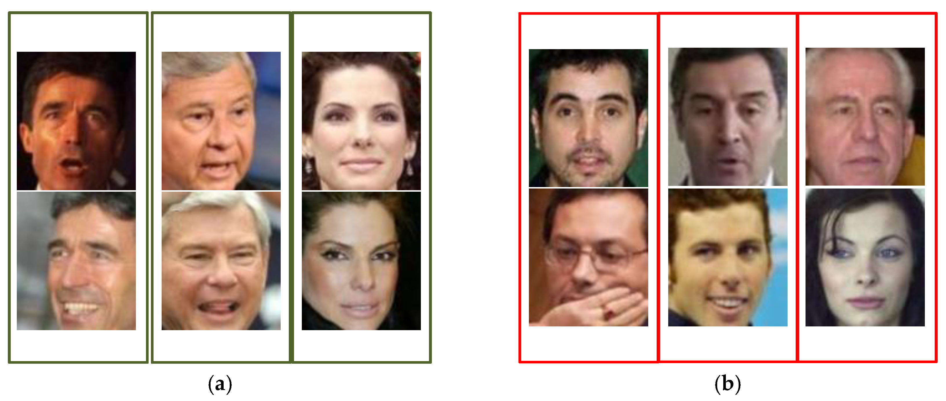
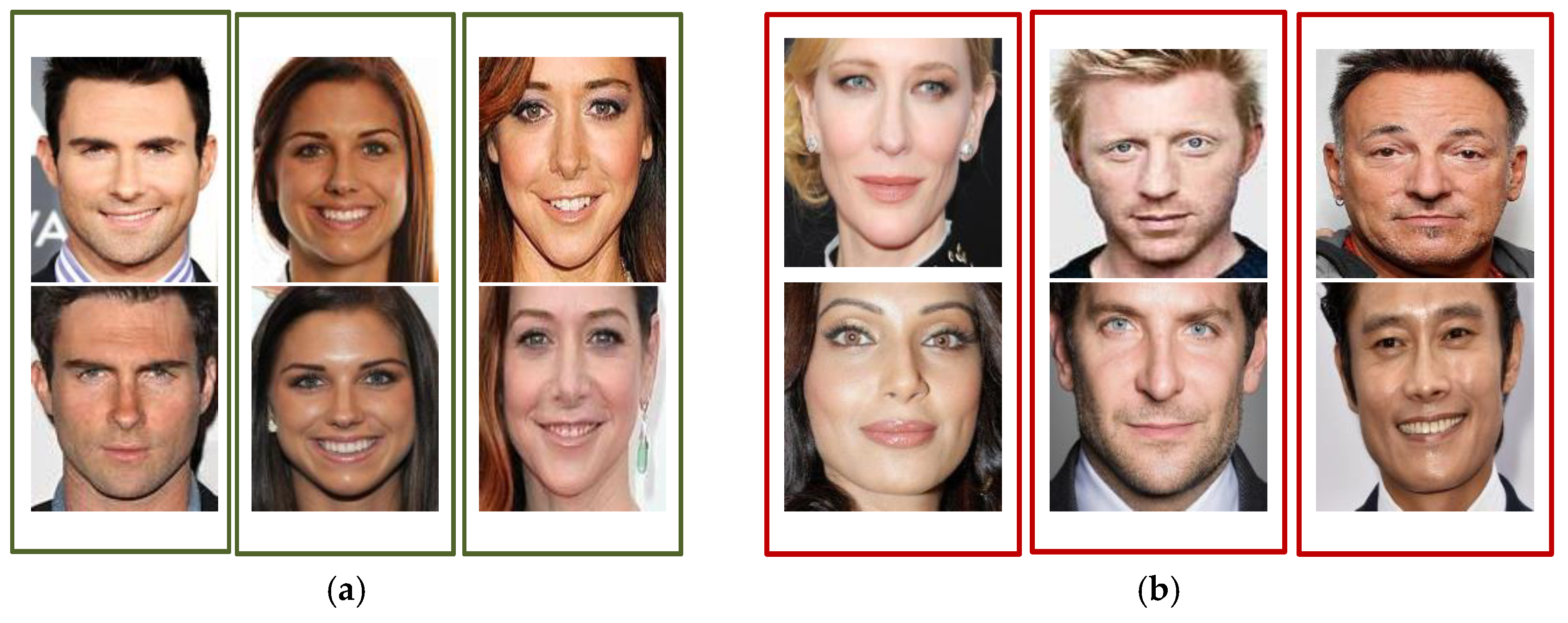
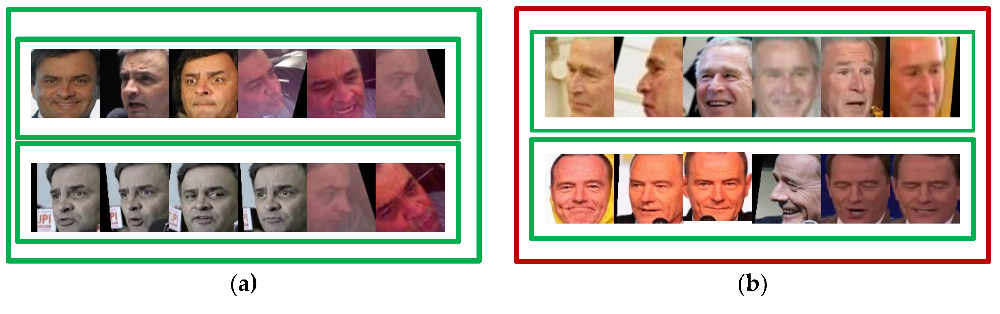
The face verification of the IJB-A dataset is different from the face verification of the LFW and the CFP datasets. The face verification of the IJB-A dataset is based on templates. The concept of a template refers to a collection of face images containing the same identity, which may come from network images or frames in a movie. Figure 14 shows the test protocol diagram.

As shown in Figure 14, the green boxes represent the same target and the red boxes represent the different targets. In Figure 14a, each row represents the face template of the same person, while the upper and lower rows belong to the face of the same person, that is, the real classification is the same target. In Figure 14b, each row represents the face template of the same person, while the upper and lower rows represent the face of the different person, that is, the real classification is not the same target. In the test, the average feature representation of the template replaces the feature representation of a single image. Then, we calculate the distance of the feature pair, use the threshold to classify and discriminate, and obtain the prediction classification. Finally, we compare the prediction with the real classification to obtain the accuracy.

Table 4. TPR of different algorithms in IJB-A face verification (1:1).

Algorithms	TPR@FPR = 0.001	TPR@FPR = 0.01
Deep-Multi-Pose [30]	-	78.76% ± -
Multi-task CNN [31]	-	78.74% ± 4.31%
PAMs [8]	71.10% ± 3.70%	84.70% ± 1.60%
DR-GAN [13]	70.3% ± 5.79%	85.70% ± 1.60%
Chen et al. [26]	74.30% ± -	87.30% ± -
PTFRM_Y	85.25% ± 0.37%	89.73% ± 0.76%
PTFRM_PYR	89.30% ± 1.39%	93.82% ± 0.78%

shows the test result of face verification (1:1).

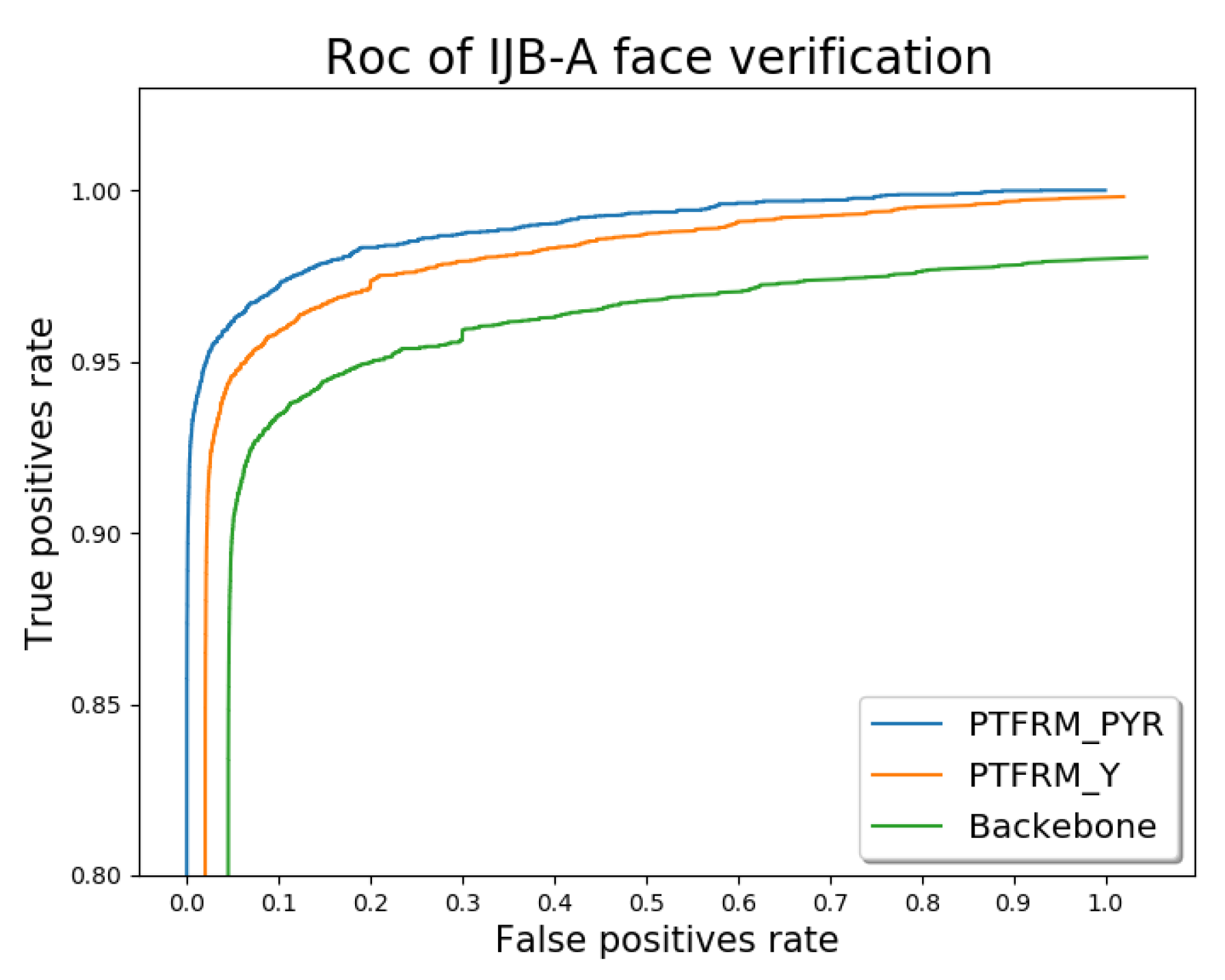
We design and compare three schemes, namely Backbone, PTFRM_Y, and PTFRM_PYR. For PTFRM_Y, only the yaw angle for depth feature transformation is taken into account. For PTFRM_PYR, the yaw, pitch, and roll are taken into account comprehensively. Figure 14 shows the receiver operating characteristic(ROC) comparison on IJB-A Face Verification (1:1) for these three schemes.

The IJB-A dataset presents additional challenges for large-angle face data. We can explore the role of the PTFRM module by comparing ROC curves and performance of different models in the IJB-A face validation(1:1).

FPR is the false positive rate, that is, the proportion of samples whose true label is negative but predicted to be positive in all samples whose true label is negative. For example, FPR = 0.001 represents 1000 negative samples, allowing one negative sample to be predicted as a positive sample. FPR = 0.001 represents 100 negative samples, allowing one negative sample to be judged as a positive sample. The scene represented by FPR = 0.001 is more stringent than 0.01. TPR stands for the true positive rate, that is, the proportion of samples whose true label is positive and predicted as positive classes in all samples whose true label is positive. In general, when the FPR is fixed, the higher the TPR, the better the network performance.

As seen from the comparison in Figure 15, we can find that the PTFRM module is a lightweight and effective component, which can be embedded in the backbone network. The PTFRM module can be used to convert the profile features in the deep network into frontal features effectively to improve the performance of face recognition. In addition, most research only considers the impact of yaw angle on facial postures. However, the comprehensive consideration of pitch, yaw, and roll can improve the performance of the PTFRM module.

4.3.2. Face Identification

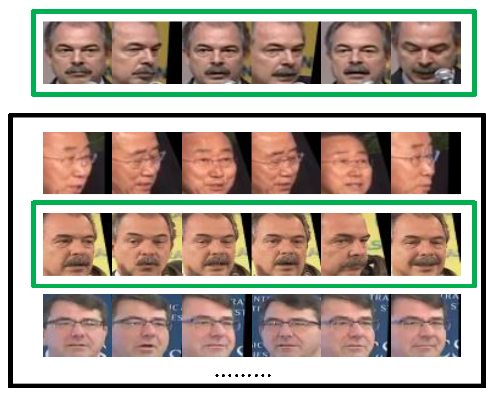
Figure 16 shows the test protocol for face recognition. The first row is the template to be tested. All images in the template are the same target. The black boxes below are all search template libraries. Among them, two green boxes are templates of the same target, and the rest are templates of different targets. During the test, we compare the template to be tested with the template in the search template library one by one. Then, we obtain a similarity list. According to the test protocol and the specific requirements of the scenario, we can find one or several targets with the highest similarity, which is predicted to be the same class as the template to be tested. Finally, we compare it with the real classification to achieve accuracy. The test results are shown in

Table 5. Accuracy of related algorithms in face recognition (1:N).

Algorithms	Accuracy@Rank = 1	Accuracy@Rank = 5
COTS matcher [24]	82.20% ± 2:3%	93.10% ± 1.4%
Deep-Multi-Pose [30]	84.60% ± -	92.70% ± -
Multi-task CNN [31]	85.80% ± 1.40%	93.80% ± 0.9%
PAMs [8]	86.20% ± 1.3 0%	94.30% ± 0.9%
DR-GAN [13]	91.0% ± 1.5%	95.6% ± 1.1%
Chen et al. [26]	87.30% ± -	93.10% ± -
PTFRM_Y	91.62% ± 0.62%	93.87% ± 0.57%
PTFRM_PYR	94.33% ± 0.84%	97.06% ± 0.64%

.

The accuracy@Rank = 1 indicates that the proportion of the templates with the highest similarity in the similarity list is the same as the template to be tested to all the templates. The accuracy@Rank = 5 that indicates the ratio of five templates with the highest similarity in the similarity list is the same as the templates to be tested in all the templates. Evidently, Rank = 1 is more demanding than Rank = 5. Table 5 shows that the accuracy of the proposed algorithm is relatively stable, and the deviation is relatively small, indicating that the stability and generalization ability of the network is strong. Given the fine classification of the three pose components at the same time, the transformation mapping ability of the PTFRM module is enhanced. Thus, we can convert complex pose facial feature representations into frontal facial feature representations. The proposed algorithm in this study is better than the comparison algorithm, especially the accuracy in the Rank = 1 scenario. Moreover, it has a greater advantage than other algorithms.

4.4. Runtime

The effect of PTFRM is demonstrated by testing the accuracy and runtime of face detection and face recognition with and without the PTFRM module. We use Intel-core i7-8700k CPU and a single GTX 1080Ti GPU to complete the experiment. One hundred images with only one face per picture are taken as an example.

Table 6. The processing speed of each model.

Model	Cost Time/100 Images
Backbone	13 s
PTFRM_PYR	14 s

shows the results.

The PTFRM_PYR model completes the feature extraction and feature comparison of a face image with 140 ms. The processing speed can reach 10 fps. After adding the PTFRM module, the runtime does not increase significantly. The test results indicate that the PTFRM is beneficial to face recognition under multi-pose conditions within the allowable computational complexity.

5. Conclusions

This study focuses on the multi-pose face recognition problem in unconstrained scenes and summarizes the principles and shortcomings of the existing methods, such as PAMs, DR-GAN, and DREAM. Based on the core idea of approximating a “frontal” image at the feature level, we propose the PTFRM module. The module maps the original feature representation by using pose labels and choosing different mapping relationships. Then, the original feature representation becomes a feature representation of the approximate “frontal” face. While maintaining the end-to-end characteristics of the network, this method has higher resource utilization and better recognition effect than other methods.