Abstract
The fine-grained image classification task is about differentiating between different object classes. The difficulties of the task are large intra-class variance and small inter-class variance. For this reason, improving models’ accuracies on the task heavily relies on discriminative parts’ annotations and regional parts’ annotations. Such delicate annotations’ dependency causes the restriction on models’ practicability. To tackle this issue, a saliency module based on a weakly supervised fine-grained image classification model is proposed by this article. Through our salient region localization module, the proposed model can localize essential regional parts with the use of saliency maps, while only image class annotations are provided. Besides, the bilinear attention module can improve the performance on feature extraction by using higher- and lower-level layers of the network to fuse regional features with global features. With the application of the bilinear attention architecture, we propose the different layer feature fusion module to improve the expression ability of model features. We tested and verified our model on public datasets released specifically for fine-grained image classification. The results of our test show that our proposed model can achieve close to state-of-the-art classification performance on various datasets, while only the least training data are provided. Such a result indicates that the practicality of our model is incredibly improved since fine-grained image datasets are expensive.
1. Introduction
Image classification is gaining increasing attention mainly for its wide use in the Internet of Things, self-driving cars, security, medical treatment, etc. People’s daily life has been changed by the use of computer-based automatic classification and recognition. Nonetheless, such usage is facing growing challenges for people who are no longer satisfied with getting coarse-grained classification results but desire finer-grained ones. Different from general object classification, which aims to distinguish basic-level categories, fine-grained image classification focuses on recognizing images that belong to the same basic category but not the same class or subcategory [1,2]. For instance, in the security domain, while monitoring vehicles passing through checkpoints, not only coarse-grained information like the types of vehicles (SUV, sedan, truck, and so on), or brand (Volkswagen, Mercedes Benz, BMW, or so) are wanted but also more accurate and fine-grained information like the models of vehicles (Volkswagen Sagitar 2006–2011, Volkswagen Sagitar 2012–2014, BMW 3 Series 2013–2014, and so on) are wanted. This finer-grained information will provide great help for case investigation, tracking accident escape, deck, and fake vehicles to traffic law enforcement departments. Hence, with this help, governments can maintain or even improve social stability. For this reason, fine-grained image classification has great research value and broad application prospects.
Fine-grained image classification is an important research topic in the field of computer vision, which aims to perform lower-level fine-grained classification upon higher-level coarse-grained categories. The main challenge of fine-grained classification is that the differences between different subcategories are usually subtle and local. In the related studies, it is usual to pre-process images for the extraction of image features, like color, texture, and contour. Then, the extracted features are used for training different models. During the test process, the same pre-processing procedure is applied to the testing images for the extraction of features, and these features are fed into the trained model to achieve classification results. Therefore, in the early stage, the bag-of-words method was first proposed [3]. Traditional artificial features are fed into the model to extract the corresponding feature vectors and obtain the final classification results. Wah et al. introduced the CUB200-2011 dataset [4] and proposed some benchmark methods. However, their classification method for uncropped images only achieved an accuracy of 10.3%. Their model was used to first locate regional areas, then apply the bag-of-words method for encoding two different kinds of feature, RGB histogram features, and scale invariant feature transform (SIFT) features [5]. The encoded features would be fed into a support vector machine (SVM) classifier for image classification training. Such low accuracy is not satisfying. This method is limited due to the regional area localization method they used being not accurate enough; also, the artificially designed features cannot distinguish enough. Hence, many researchers have proposed new feature descriptors based on their research, like part-based one-vs-one features (POOF) [6], Fisher-encoded SIFT [7], supervised kernel descriptors for visual recognition (KEDS) [8], etc. These methods, on fine-grained image classification, can reach an accuracy from 50% up to 62% [9,10].
From the early model design, we can see that the use of discriminative extracted image features and feature encoding methods have a significant impact on the final classification results, which means the better the methods that are used, the more discriminative features are used, and the better the classification results. So, it can be seen that locating the regional feature area of images plays an important part in achieving good classification results. However, annotating the regional feature area manually is expensive, resulting in obvious defects on practical applications.
In recent years, deep neural networks have been widely used in the field of computer vision. According to the annotations used during training, deep neural network methods are divided into strongly supervised learning [11,12,13,14,15] and weakly supervised learning [16,17,18]. The strongly supervised fine-grained image classification method is characterized by not only image category tag data but also additional manual annotations, such as key points of annotations or regional area annotations that are provided during training. Thus, strongly supervised fine-grained image classification methods require additional manually annotated data, which makes these methods expensive and heavily restricts their application area. For these reasons, strongly supervised methods may not be the most appropriate choice for the actual classification tasks. Adopting the weakly supervised method is another big trend in the field of fine-grained image classification research. How to find the most discriminative regions has been studied by various researchers.
A weakly supervised fine-grained classification network based on two-level attention is proposed by this article for tackling this problem. Our method consists of two parts. One of them is based on salient region localization module. This module is designed for locating discriminative regions, and it is trained while only using images’ categories as labels. The other one is the bilinear attention module for fusing regional and global features. This module is used for extracting regional and global feature from higher- and lower-level layers of bilinear neural networks separately. Then, we fuse these features to improve the features’ representation capability and construct our different layer feature fusion module. The main contributions of our study are as follows:
- The differences between different subcategories are usually subtle and local. Hence, how to locate and distinguish the area has become key to solving the problem. An essential new regional area localization method (salient region localization module) is proposed, which can accurately locate and extract the most distinct regional areas and reduce the dependence of manual annotation information.
- We adopt the bilinear neural network for the extraction of global features and regional features, which allows us to make better use of global features and regional features for training. The use of the bilinear neural network allows us end-to-end train our model. Besides, using bilinear neural network makes our model more stable.
- Due to huge intra-class variance and small inter-class variance, a different layer feature fusion module is proposed. First, we add center loss to our loss function to improve the distinction between classes. In this way, we can reduce the impact of large intra-class variance and small inter-class variance. Finally, we better guide the fine-grained image classification by combining low-level visual features and advanced semantic information.
- Our resulted model is trained without providing manually annotated essential areas while reaching an accuracy of 85.1% on the CUB-200-2001 dataset. Our method’s resulting accuracy is better than most strongly supervised method ones. This result shows that our model can reduce the dependence on delicate manually annotated essential areas while maintaining acceptable accuracy.
The rest of this article is organized as follows. We first review the techniques related to the two-level attention module, applications of the saliency module in weakly supervised image classification, and the different layer feature fusion method in Section 2. Section 3 introduces our proposed network architectures for fine-grained image classification. To verify the effectiveness of our method, extensive experiments are performed in Section 4. The conclusion and future works are summarized in Section 5.
2. Related Works
The key to image classification is to extract the robust features of the object and form a better feature representation. From the relevant studies, we can find that adding a weakly supervised method to fine-grained image classification is a big trend in recent years. The application of the weakly supervised method is mainly for reducing dependency upon delicate manual labels, especially manually annotated essential areas. In order to apply the fine-grained classification methods to actual tasks, many researchers have studied how to accurately locate and distinguish salient regions under weakly supervised conditions, and then use Convolutional Neural Network (CNN) to extract features from these detected regions. Previous work on fine-grained classification usually focused on part detection to establish correspondence between object instances and reduce the impact of object posture changes under strictly supervised settings.
2.1. Two-Level Attention Model
The attention mechanism has the ability to pay attention to certain content while ignoring other content. The ITTI model introduced the attention mechanism for the first time, where it was used for saliency detection [19]. Dzmitry employed a single-layer attention model to solve the problem of machine translation [20]. The inception series expanded the width of the CNNs to achieve adaptability to different convolutional scales [21,22,23]. Xiao et al. made an initial attempt at introducing a weakly supervised method to fine-grained image classification [24]. The two-level attention module they proposed is capable of casting attention on two different level features, which is similar to the object-level and part-level feature of the strongly supervised learning method. The bilinear CNN (B-CNN) model was proposed by Lin et al. for the reduction of redundancy caused by the candidate region extraction algorithm [25]. Similar to the two-level attention model, our model is built based on the bilinear convolutional neural network.
2.2. Saliency Module in Weakly Supervised Image Classification
Peng et al. mentioned two basic concepts [1]: One is a collection of all feature maps for the same convolutional layer, collectively referred as the "activation set", and the other is that an activation set can be represented by a T-dimensional vector, which is called the “descriptor”. The method proposed by Peng et al. is heavily influenced by hyperparameters, which makes their model very unstable and hard to reproduce. Besides, their model is not end-to-end, which reduces its practicality. When using a convolutional neural network for training, all feature maps of different depths of the convolutional layer or feature maps in the same depth of the convolutional layer have different responses toward the same image. Such a phenomenon is shown in Figure 1. The figure is from research produced by Selvaraju et al. [26]. Therefore, making better use of each feature map will improve the performance of the model for image classification. We use the weighted gradient-based algorithm for class activation mapping in our method for this reason. This process is inspired by the process used in gradient class activation mapping (Grad-CAM), which was proposed by Selvaraju et al. [26]. This process enables us to eliminate the influence brought by different structures of convolutional neural networks.
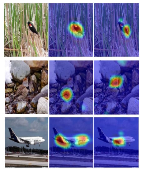
Figure 1.
The figure above shows feature maps from different channels, generated with the Class Activation Mapping via Gradient-based Localization (Grad-CAM) method by Selvaraju et al. [26]. From the figure above, we can see that Grad-CAM can easily locate salient places of different images. Heat maps from different channels generated in this way have various focusing points. We use these heat maps to extract regional features.
2.3. Different Layer Feature Fusion
Since different layers of convolutional features describe the characteristics of objects and their surroundings from different angles, how to obtain low-level visual features while considering high-level semantic information has become a new research hotspot in the field of image processing. Hariharan et al. achieved better fine-grained segmentation, object detection, and semantic pixel segmentation by aggregating low-level features with high-level features [27,28,29]. Jin et al. proposed the use of a recurrent neural network to transfer high-level semantic information and low-level spatial features to each other for the analysis of scene images [30]. Based on the saliency module and low-level attention module, due to huge intra-class variance and small inter-class variance, this paper combines the attention features of multiple intermediate layers and delivers them layer by layer. Finally, we better guide the fine-grained image classification by combining low-level visual features and advanced semantic information.
3. Approach
The characteristics of fine-grained images are large intra-class variance and small inter-class variance. The bilinear convolutional neural network can better pay heed to the regional features of the images. Additionally, it has the capability of learning regional features, hence it is capable of representing the relationship between regional features. What is more, it is capable of end-to-end training without manual intervention.
We choose to use bilinear CNN as our baseline feature extraction neural network. We use features from a high level and lower level of the network to calculate outer products, which are later used as image features. Our model is based on the weakly supervised learning method. For this reason, we can only use image class labels for training our model while not providing manually annotated essential regional areas during our training process. By doing so, our proposed model reduces the dependence on artificial annotation. The overall structure is illustrated in Figure 2. Our model is composed of three parts.
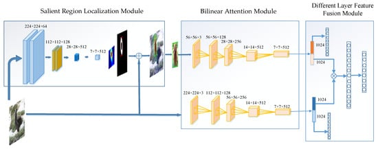
Figure 2.
Overview of our neural network’s structure. The whole neural network is a two-level attention model. The saliency module is used for locating salient regions of the target images, then the bilinear attention module is used as our feature extractor. Finally, the derived features are used to calculate the outer product to achieve the final fused feature.
First, the salient region localization module, which is used for locating salient regions of the target images. The salient regions would be intercepted as the input to the first layer of the bilinear CNN.
The second part is the bilinear attention module, which serves as a feature extractor. The extracted feature maps from this model are used as the parallel input of the maximum pooling layer and average pooling layer, that is, each feature map is converted into two vectors, one containing maximum values and the other containing average values. These vectors are used as descriptor vectors.
The third part is the different layer feature fusion module, calculating the outer product of features extracted from the higher level and lower level of the network for fusion. Then, the fused features are fed into the softmax classifier. During the training process, we construct an auxiliary mixed loss function for better integration of the regional features and global features.
3.1. Salient Region Localization Module
Our model uses bilinear CNN to extract features. Then, a weighted gradient-based algorithm for class activation mapping is applied on the resulting features. This process is inspired by the process used in the Grad-CAM model, which was proposed by Selvaraju et al. [26]. This process enables our model to eliminate the influence brought by varying structures of convolutional neural networks. Additionally, it grants our model the ability to generate visually interpretable feature maps. It also makes our model capable of giving a score to a specific label when only one image and the target labels are fed into our bilinear CNN model without training from the ground up or changing the original CNN model’s structure. The score of the labels is obtained through the calculation of specific tasks. For all labels, except the required, the labels’ gradients are set to 1; the rest of the gradients are set to 0, and then the gradient is propagated back to the entire convolutional feature map. All feature maps are combined by a precise method for obtaining heat maps of the given image. The resulting heat map reveals the part that needs to pay more attention. Finally, we apply element-wise multiplication to the heatmap and the directed backpropagation, using bilinear interpolation to up-sample the input image’s resolution. Then, we merge the backpropagation results and visualization results to obtain saliency maps, which are shown in Figure 3.
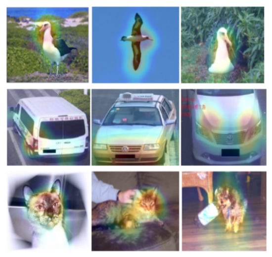
Figure 3.
Saliency maps of different images.
After obtaining the generated saliency map, an adaptive maximum inter-class variance algorithm is used to obtain the threshold according to the calculation [31], and the threshold is used for converting the saliency feature map into a binary mask. Thereby, we can distinguish the background from the foreground and highlight the differences between these two parts of the image. We use “1” for meaning the specific position of the provided image is foreground, and “0” for meaning that the position is background. Then, we apply the eight-connected region labelling algorithm to the foreground to locate the target and label the target coordinates. The mentioned processes of the saliency model are shown in Figure 4.
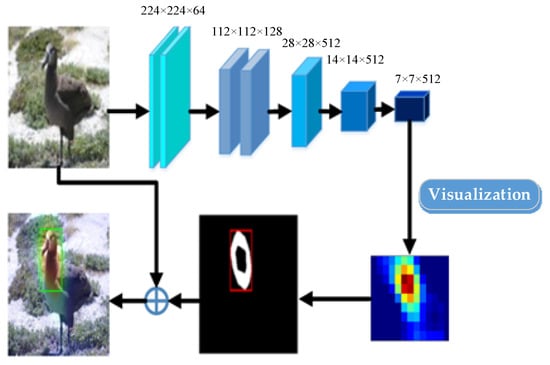
Figure 4.
Saliency module based on weakly supervised learning.
We locate and obtain the most distinct regional area from the input image to generate the heat map. We choose to generate heat maps as they can be visualized directly by adding to the original image. We use the bilinear interpolation method to generate a heat map for the original image. The heat map and the input image have the same size. The heat map will be combined with the original image.
However, different feature maps have a different region of response on original images, and the key regional features are found to be not salient enough after visual analysis, so we cannot localize salient targets with them. To solve this problem, we decide to sum over the d dimension of three-dimension tensor D, which has the size , turning it into a two-dimension tensor B, which has the size , to better localize salient targets. The addition equation is as follows:
In the equation above, is a feature map of the i-th channel. The fusion of multiple feature maps through Equation (2) helps our model to enhance the feature information of salient areas, which in turn makes it easier to locate regional salient areas more accurately. Each saliency map, having the size of , corresponds to all pixels in the area. We also calculate a self-adaptive threshold, , using the OTSU algorithm [32]. With the derived threshold, we can turn a saliency map into a binary map; the equation is as follows:
For the processed binary image , we perform a scan, and mark all pixels’ connection areas according to the four-neighborhood rule. It is assumed a pixel is represented by , where the produces the binary value of the pixel by , , which stand for the pixel’s location in image. And we assume the connectivity domain tag of pixel is represented by . When scanning , the scanning process is already done for and , so their marks, and , are already known. Hence, the connected area mark of the pixel is only relevant to the connected area marks of pixel and , which are and . The equation is as follows:
In the equation above, when the condition to the right of Function (3) holds, the marker number of the connection mark is the same. At the same time, in the final case of Function (3), if the condition is true that pixel belongs to the new connection domain, . Additionally, we set the value of to the value of the new connected area mark Newlabel.
To better visualize the effect of the salient region localization module, we plot the bounding box based on the resulting detected saliency regions. As shown in Figure 5, we visualize the effect of the module on different fine-grained datasets. We can see that even for different fine-grained images, all the regions of focus are detected accurately. Especially, most parts of the response will be in the foreground of the target to be classified, and only a minority will be on the background of the target to be classified.
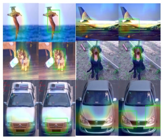
Figure 5.
Saliency localization map of different images.
3.2. Bilinear Attention Module
In this module, we adopt the general purpose bilinear neural network method, which was proposed by Lin et al. [24]. Their neural network can be mainly divided into the upper and lower level. Each level uses the VGG neural network as a feature extractor. Images are fed into the upper and lower network for the extraction of features. After that, the bilinear pooling function is performed on these extracted features to combine these features. In the end, the combined feature is fed into the Softmax layer for classification. Our model is based on the bilinear neural network. We propose a new module, the bilinear attention module, which is shown in Figure 2. This module uses the upper-level network Net-A to extract regional salient areas’ target feature , and uses the lower-level network Net-B to extract the global target feature . Then, the outer product is performed on these features to get the bilinear feature . Then, we perform the outer product again to get the bilinear feature . The outer product is calculated with the following equation:
Feature B1 is obtained by performing the dot product on and . and are features extracted from the upper- and lower-level networks’ convolutional layer separately. Feature B2 is obtained by performing the dot product on and . and are features extracted from the upper- and lower-level networks’ convolutional layer separately. Since the bilinear feature is a three-dimensional matrix with various sizes on each dimension, we need to transform the two bilinear features into column vectors. Then, we concatenate these two resulting column vectors into the new column vector B to enhance the relevance between each layer’s features, so that we can fuse the regional and global features better. In the end, we feed the resulting column vector B into the different layer feature fusion module for further processing.
3.3. Different Layer Feature Fusion Module
In this section, we will design a new layer fusion method to ensure that both the low-level visual features and high-level semantic information are fully utilized. We perform a simple convolution operation on each module in the network and combine them with the feature maps on the main path to perform fine-grained image classification.
The Softmax function is widely used for constructing the loss function in image classification. However, Softmax does not require intra-class compactness and inter-class separation, which is highly unsuitable for fine-grained classification. Therefore, to use the loss function to force our model to learn features with larger inter-class and smaller intra-class distances, we add the center loss function to improve the distinction between classes. Center loss will learn the centers of each class feature and reduce intra-class variation for each feature according to their corresponding class centers. In this way, we can reduce the impact of large intra-class variance and small inter-class variance. The definition of the center loss function is as follows:
In the equation above, stands for the center of the -th feature. During each iteration, only class centers relevant to the features are updated. The Softmax function consists of three parts: The loss function for the upper regional feature classification network, loss function for the lower global feature classification network, and fusion loss function P. Therefore, our loss function for the model is defined as follows:
In the equation above, stands for the possibility on each category, which is produced by the main neural network; is one hot encoded vector for stating each image’s label; and are the probability on each category produced by the higher-level neural network and lower one ; stands for the central feature of the i-th category; stands for the features of the input images; and and stand for the weight of each module. Hyperparameters and are chosen based on the cross-validation method, while parameter is set to 1. During the experiment, we adjust the different weights to optimize the features extracted from each layer of the bilinear network, to optimize the identification results of the entire model. Then, we set the weighting constant , , and . With the loss function above, the regional and global features of the image can be better used, which allows us to obtain a higher classification accuracy.
4. Experiments
In this section, we conduct several experiments to evaluate the performance of our models on the fine-grained image classification task. Our experiments are based primarily on public fine-grained image datasets. First, under the same hardware and software conditions, we compared the results derived from using different higher- and lower-level network loss functions, the fused loss function, and the central loss function for correlation comparison. The experiments to prove the validity of the loss function were verified in two main ways. On the one hand, by verifying the effect of an increase in the loss term on the final classification accuracy. On the other hand, by verifying whether increasing the effective loss term can speed up the convergence of the overall loss function and steer the overall loss function toward the right direction for convergence. Second, we compared the results obtained by using a single network and the bilinear network to demonstrate the effectiveness of our network. Third, to prove the advances of our network, we also compared our method with fresh relevant methods.
4.1. Datasets’ Settings
The CUB-200-2001 dataset, a few sample images of which are illustrated in Figure 6, has been extensively used in the research of fine-grained image classification [4]. The CUB-200-2001 dataset contains 11,788 images of birds, with 200 types of birds in general. Each has a different posture, which results in large intra-class variance and small inter-class variance. Differences between classes are normally small and regional, such as the beak, the color of the wings, or another regional area. The dataset not only provides classification labels for all bird image data but also provides essential part annotations. However, our method only uses a weakly supervised method, so only image label data was used in the model for training and testing. We used 70% of the data as a training set and 30% for testing.
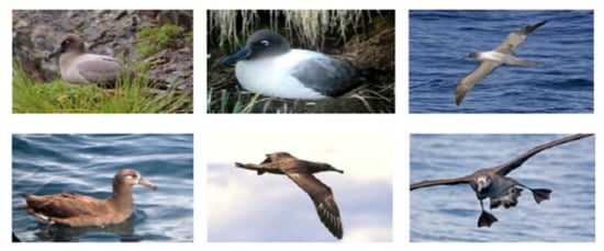
Figure 6.
Sample images from the CUB-200-2001 dataset.
The Stanford Dogs dataset provides images of data for 120 different types of dogs [33]. There are 20,580 images in total, including different perspectives and poses. Only target frame information is provided, and key point information is excluded. The sample image data are presented in Figure 7. In the figure, two distinct dog breeds are shown. From the analysis of the pictures, the backgrounds of such a dataset are complicated, as some backgrounds are set on sofa, grass, etc. Hence, when we used the Stanford Dogs dataset, in the data pre-processing stage, we cropped images according to the provided label box to reduce the impact of the responsible background. Moreover, dogs of different breeds in this type of dataset have large intra-class differences. We used 70% of the data as a training set and 30% for testing.
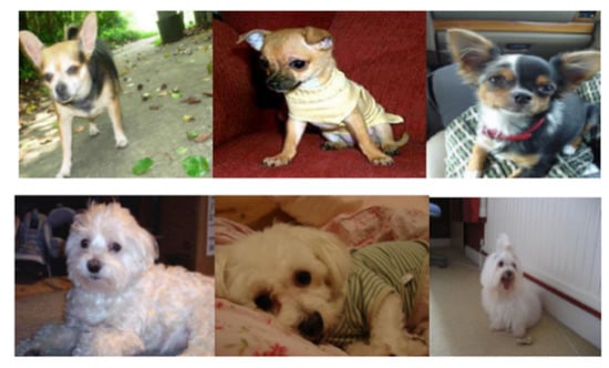
Figure 7.
Sample images from the Stanford Dogs dataset.
The FGVC-Aircraft provides image data of 102 categories of aircraft [34]. Each category has more than 100 diverse images. There are 10,200 images in total, and only label box information provided. Sample images are presented in Figure 8. We also applied image cropping to such a kind of dataset during our data pre-processing stage. We cropped the image according to the label box to reduce the impact of the background. We used 80% of the data as a training set and 20% for testing.
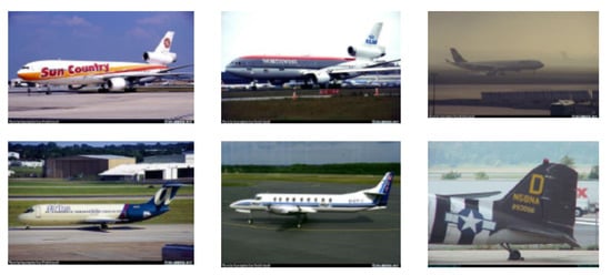
Figure 8.
Sample images from the FGVC-Aircraft dataset.
We used a subset of the CompCars dataset, which was proposed by Yang et al. [35], and contains 300,000 images of 500 categories of vehicles. We used 15 categories of vehicle type, 55 categories of vehicle brands, and 250 types of vehicle models. Each type of vehicle has approximately 300 images, covering rainy days, nights, foggy days, and different angles of view. We used 70% of the data as a training set and 30% for testing. The visualization of the CompCars dataset is shown in Figure 9.
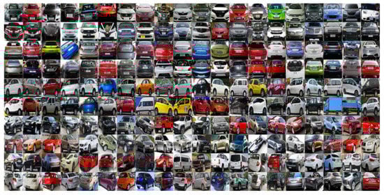
Figure 9.
Sample images from the CompCars dataset.
4.2. Data Pre-Processing
In general, whether the data can be pre-processed effectively affects the final effect of the model to a certain extent. For the case of only a few fine-grained image samples being available, we pre-processed all available images (denoising, dimension reduction, normalization, standardization etc.) and applied data expansion to avoid over-fitting.
4.2.1. Scale Cropping
Different fine-grained image datasets have different image sizes. However, the presence of the Region of Interest (ROI) pooling layer allows any size image to be fed into the deep neural network. Inspired by the idea of migration learning, we used the Inception v3 model that was pre-trained on ImageNet data. For the input image, it needs to be cropped to the image size that Inception v3 requires for input, which is . To a certain extent, it is possible to reduce the amount of data used for training, and the fixed size of the image allows the convolutional neural network to better extract the characteristic information from it.
4.2.2. Data Augmentation
To improve the classification accuracy and prevent overfitting, considering the huge amount of network parameters, we need to adopt data augmentation for an increasing amount of data. In our experiment, we used several methods to augment data from fine-grained image datasets, making the number of training samples for each category relatively balanced. The methods we used included randomly flipping and distorting images, randomly cropping images, randomly adding noise, randomly modifying the contrast and saturation of images, etc.
4.3. Comparison of Different Experiments
4.3.1. Evaluation Index
For the mentioned datasets, to better compare the performance of different algorithm models, we used the classification accuracy as the evaluation index, and it is defined as follows:
where n stands for the total number of test samples and stands for the number of images predicted correctly. Such an evaluation index can more intuitively reflect the classification performance of the models.
4.3.2. Comparative Experiment of Different Loss Functions
To confirm the validity of the loss functions, we designed the comparative experiment using the CUB-200-2001 dataset and compared the changes of the loss values of the functions when the number of iterations increased. The experimental results are shown in Figure 10, where the behavior of the different loss function is reported. The green curve refers to only the first term of the mixed loss function proposed in this paper. The blue curve represents the addition of the auxiliary function to the upper-layer network. It can adjust the upper-layer network to make it more focused on the regional feature information while enabling the model to converge faster and lower the overall loss value. The pink curve indicates the addition of the auxiliary classifier term in the lower-layer network, which allows the lower-layer network to adjust its extracted global features. Since the global features extracted by the lower-layer network have more abundant characteristic information than the regional features, the loss value is decreased more, and the classification accuracy is increased. The remaining curve, the orange one, is the variation curve of the mixed loss function proposed by this paper. The loss value of the model in the training process is close to 0. At the same time, in this curve, we can see a significant downward trend in the loss values and a significant increase in the rate of convergence. In addition to adding two auxiliary classifiers, the central loss function is added to reduce the intra-class variance and increase the inter-class variance. Additionally, the results in Table 1 show that the accuracy of the identification can be effectively improved.
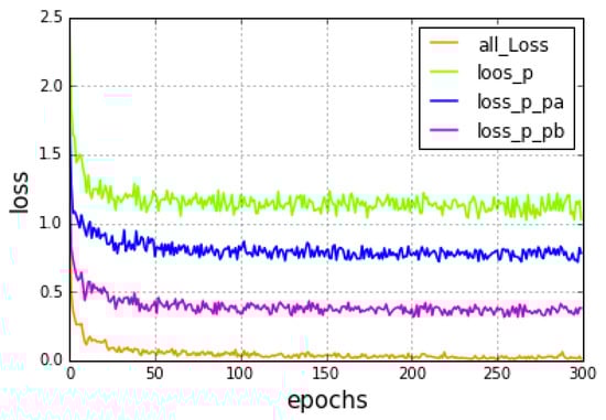
Figure 10.
Loss values of the different loss function.

Table 1.
Accuracy of different loss functions.
In the test partition of the CUB200-2011 dataset, there were approximately 20 images for each category. We compared obtained accuracies of the model using different loss functions, and chose to set and . The results are shown in Table 1. The accuracy of the model proposed in this paper reached 84.12% on public datasets. This result is better than some strong supervised learning methods and some weakly supervised learning methods mentioned in the related works in the first chapter.
4.3.3. Classification Results of Different Network Structure
The basic network structure of the model proposed in this paper is based on Inception v3. For this reason, in our experiments, we used the parameters from the Inception v3 model pre-trained on the ILSVRC2012 dataset to initialize our model’s parameters. For the CUB200-2011 dataset, we used a single network structure to classify fine-grained images, such as Inception v3 and DenseNet.
For the bilinear model, we used B-CNN proposed by Lin et al. [25]. The experimental results are shown in Figure 11. Although the single network structure can improve the accuracy of image classification to some extent when increasing the depth of the network, its performance is still weaker than the bilinear model. Hence, we can derive the conclusion that the bilinear deep neural network can make better use of the relationship between regional features and global features. At the same time, our method runs with only 5M parameters, while achieving a classification speed of 48 frames per second. From the derived experimental results, our proposed method obtained a better performance than B-CNN, reaching a classification accuracy of 85.1%.
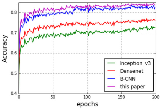
Figure 11.
Accuracies of different networks on the CUB200-2011 dataset.
4.3.4. Comparison of State-of-the-Art Algorithms
We intended to prove that our model is more versatile and advanced in different fine-grained datasets. Therefore, we compared our method in the different datasets, CUB-200-2001, Stanford Dogs, and FGVC-Aircraft, with current state-of-the-art methods. Considering the existing methods have significant differences in the performance on different datasets, we chose to use the classification results on the corresponding datasets recorded in the relevant papers during our comparison. The comparison results are shown in Table 2, Table 3 and Table 4.
Table 2.
Classification accuracy on the FGVC-Aircraft dataset.
Table 3.
Classification accuracy on the Stanford Dogs dataset.
Table 4.
Classification accuracy on the CUB 200-2011 dataset.
Because the CUB200-2011 dataset provides essential points data, when we compared the performance on the dataset, we chose to compare our method with strongly supervised methods. Table 5 shows the classification labels of some of the images in the CUB 200-2011 dataset by advanced methods. The text in red indicates an incorrect classification result. As we can see from the typical test images, without the corresponding injection of manually supervised information, our classification remains accurate for images with small inter-class differences and large intra-class differences. Additionally, there are fewer instances of classification failures due to differences in the perspective and background.
Table 5.
Test image results on the CUB 200-2011 dataset: the red text represents misclassification.
From the tables above, we can see that our method has a great performance on the Stanford Dogs and FGVC datasets; also, our method reaches an accuracy of 85.1% on the CUB-200-2001 dataset, which is better than some strongly supervised algorithms, indicating that weakly supervised methods can reduce the dependence on manual data labelling and improve the practicability of the algorithm while ensuring a certain accuracy. Our accuracy is higher than the OPAM proposed by Peng et al. on the FGVC-Aircraft dataset [1]. On the CUB 200-2011 dataset, our accuracy is very similar to the OPAM method proposed by to Peng et al. However, OMPA runs with roughly 35M parameters, which is seven times the number we used, and only achieves a classification speed of 4 frames per second. We reduced the number of parameters while increasing the speed of detection and ensuring classification accuracy.
To verify that the proposed model has good performance on the challenges faced in the project, we also tested our model on the CompCars dataset.
To compare the classification results of different vehicle hierarchy features, the existing vehicle labels were divided into three hierarchical labels according to the vehicle hierarchy division method. Since the dataset we used is not a public dataset, we reproduced some related algorithms for fine-grained image classification on our dataset. Through the experimental comparison, it can be known that in the case of large classification labels, each method has a good performance, and the highest accuracy is up to 98.35%, and the accuracy of the model proposed in this paper is close to the state-of-the-art one. When the image label is configured as the vehicle brand, the classification accuracy decreases as the category to be classified increases. The proposed model has better stability and has a little decrease in accuracy. Under the third level of 250 types of vehicle model labels, all algorithms have a significant decrease in accuracy. It can be seen from Table 6 that through the experimental comparison, the classification accuracy of the proposed model reached 90.56%, which is on the brink of the latest classification accuracy results reported on CVPR obtained by Fang et al. [41], indicating that the model proposed in this paper has certain superiority and practicability. At the same time, the evaluation and metrics for the model in Fang et al. were optimized for the CompCars data set only. In contrast to the deeper experiments above, we compared the results on multiple datasets to make sure our model is not optimized for a specific dataset. Besides, we aimed to show that our proposed method retains the advantages of end-to-end training and testing by adopting bilinear neural networks. Thus, the generality and superiority of our proposed algorithm is shown in the test results from multiple data sets.
Table 6.
Different levels of vehicle label recognition results.
5. Conclusions
Our survey aimed to study the small inter-class variance and large inter-class variance characteristic of fine-grained image data, and the dependence of labels. Based on our study, we proposed a new method, which is based on the weakly-supervised learning method and saliency module, for fine-grained image classification. The salient region localization module first extracts salient regional area information. Then, the information is fed into the bilinear attention module. The higher-level layer of the bilinear neural network is used for extracting the regional feature, while the lower-level one is used for extracting global feature. Fused features are extracted by calculating the outer product on features acquired from higher- and lower-level layers, which can be utilized to construct the auxiliary hierarchical mixed loss function. The different layer feature fusion module allows the neural network to better fuse regional features and global features. The experimental results show our model can achieve great classification results on various datasets, which demonstrate our model’s robustness.
In the future, we will mainly focus on improving the classification accuracy while having hundreds of, thousands of categories to predict, for realizing end-to-end classification. Additionally, the method proposed in this paper is based on the weakly supervised learning method, which allows our model to accurately locate and extract the most distinct regional areas, and reduces the dependence of manual annotation information.
Author Contributions
Methodology, F.C., and G.H.; Writing—original draft, F.C., J.L., and Y.W.; Writing—review and editing, J.L., G.H., C.-M.P., and W.-K.L.; Supervision, C.-M.P., and W.-K.L.; Funding acquisition, L.C. All authors have read and agreed to the published version of the manuscript.
Funding
This work was supported in part by the National Natural Science Foundation of China under Grant 61702111, the National Nature Science Foundation of China-Guangdong Joint Fund under Grant 83-Y40G33-9001-18/20, the National Key Research and Development Program of China under Grant 2017YFB1201203, the Guangdong Provincial Key Laboratory of Cyber-Physical System under Grant 2016B030301008, the National Natural Science Foundation of Guangdong Joint Fund under Grant U1801263, the National Natural Science Foundation of Guangdong Joint Fund under Grant U1701262, the Guangdong R&D plan projects in key areas under Grant 2019B010153002, the Guangdong R&D plan projects in key areas under Grant 2018B010109007, the “Blue Fire Plan” (Huizhou) Industry-University-Research Joint Innovation Fund 2017 Project of the Ministry of Education under Grant CXZJHZ201730, and the Guangdong R&D plan projects in key areas under Grant 2019B010109001.
Conflicts of Interest
The authors declare no conflict of interest.
References
- Peng, Y.; He, X.; Zhao, J. Object-Part Attention Model for Fine-Grained Image Classification. IEEE Trans. Image Process. 2018, 27, 1487–1500. [Google Scholar] [CrossRef] [PubMed]
- Luo, J.-H.; Wu, J.-X. A survey on fine-grained image categorization using deep convolutional features. Acta Autom. Sin. 2017, 43, 1306–1318. [Google Scholar]
- Zhang, L.-B.; Wang, C.-H.; Xiao, B.-H.; Shao, Y.-X. Image Representation Using Bag-of-phrases. Acta Autom. Sin. 2012, 38, 46–54. [Google Scholar] [CrossRef]
- Wah, C.; Branson, S.; Welinder, P.; Perona, P.; Belongie, S. The Caltech-UCSD Birds-200-2011 Dataset; CNS-TR-2011-001; California Institute of Technology: Pasadena, CA, USA, 2011. [Google Scholar]
- Abdel-Hakim, A.E.; Farag, A.A. CSIFT: A SIFT Descriptor with Color Invariant Characteristics. In Proceedings of the 2006 IEEE Computer Society Conference on Computer Vision and Pattern Recognition (CVPR’06), New York, NY, USA, 17–22 June 2006; pp. 1978–1983. [Google Scholar]
- Berg, T.; Belhumeur, P. Poof: Part-based one-vs.-one features for fine-grained categorization, face verification, and attribute estimation. In Proceedings of the IEEE Conference on Computer Vision and Pattern Recognition, Portland, OR, USA, 23–28 June 2013; pp. 955–962. [Google Scholar]
- Perronnin, F.; Sánchez, J.; Mensink, T. Improving the Fisher Kernel for Large-Scale Image Classification. In European Conference on Computer Vision; Springer: Berlin/Heidelberg, Germany, 2010; pp. 143–156. [Google Scholar]
- Wang, P.; Wang, J.; Zeng, G.; Xu, W.; Zha, H.; Li, S. Supervised kernel descriptors for visual recognition. In Proceedings of the IEEE Conference on Computer Vision and Pattern Recognition, Portland, OR, USA, 23–28 June 2013; pp. 2858–2865. [Google Scholar]
- Branson, S.; Van Horn, G.; Wah, C.; Perona, P.; Belongie, S. The Ignorant Led by the Blind: A Hybrid Human–Machine Vision System for Fine-Grained Categorization. Int. J. Comput. Vis. 2014, 108, 3–29. [Google Scholar] [CrossRef]
- Chai, Y.; Lempitsky, V.; Zisserman, A. Symbiotic segmentation and part localization for fine-grained categorization. In Proceedings of the IEEE International Conference on Computer Vision, Sydney, Australia, 1–8 December 2013; pp. 321–328. [Google Scholar]
- Deng, J.; Krause, J.; Fei-Fei, L. Fine-grained crowdsourcing for fine-grained recognition. In Proceedings of the IEEE Conference on Computer Vision and Pattern Recognition, Portland, OR, USA, 23–28 June 2013; pp. 580–587. [Google Scholar]
- Xu, Z.; Huang, S.; Zhang, Y.; Tao, D. Augmenting strong supervision using web data for fine-grained categorization. In Proceedings of the IEEE International Conference on Computer Vision, Santiago, Chile, 7–13 December 2015; pp. 2524–2532. [Google Scholar]
- Zhang, N.; Donahue, J.; Girshick, R.; Darrell, T. Part-based R-CNNs for fine-grained category detection. In Proceedings of the European Conference on Computer Vision, Zurich, Switzerland, 6–12 September 2014; pp. 834–849. [Google Scholar]
- Lin, D.; Shen, X.; Lu, C.; Jia, J. Deep lac: Deep localization, alignment and classification for fine-grained recognition. In Proceedings of the IEEE Conference on Computer Vision and Pattern Recognition, Boston, MA, USA, 7–12 June 2015; pp. 1666–1674. [Google Scholar]
- Branson, S.; Van Horn, G.; Belongie, S.; Perona, P. Bird Species Categorization Using Pose Normalized Deep Convolutional Nets. In Proceedings of the BMVC 2014—British Machine Vision Conference, Nottingham, UK, 1–5 September 2014. [Google Scholar]
- Simon, M.; Rodner, E. Neural activation constellations: Unsupervised part model discovery with convolutional networks. In Proceedings of the IEEE International Conference on Computer Vision, Santiago, Chile, 7–13 December 2015; pp. 1143–1151. [Google Scholar]
- Wang, D.; Shen, Z.; Shao, J.; Zhang, W.; Xue, X.; Zhang, Z. Multiple granularity descriptors for fine-grained categorization. In Proceedings of the IEEE International Conference on Computer Vision, Santiago, Chile, 7–13 December 2015; pp. 2399–2406. [Google Scholar]
- Jaderberg, M.; Simonyan, K.; Zisserman, A. Spatial Transformer Networks, Advances in Neural information Processing Systems; MIT Press: Montreal, QC, Canada, 2015; pp. 2017–2025. [Google Scholar]
- Mnih, V.; Heess, N.; Graves, A. Recurrent Models of Visual Attention, Advances in Neural Information Processing Systems; MIT Press: Montreal, QC, Canada, 2014; pp. 2204–2212. [Google Scholar]
- Bahdanau, D.; Cho, K.; Bengio, Y. Neural machine translation by jointly learning to align and translate. arXiv 2014, arXiv:1409.0473. [Google Scholar]
- Szegedy, C.; Liu, W.; Jia, Y.; Sermanet, P.; Reed, S.; Anguelov, D.; Erhan, D.; Vanhoucke, V.; Rabinovich, A. Going deeper with convolutions. In Proceedings of the IEEE Conference on Computer Vision and Pattern Recognition, Boston, MA, USA, 7–12 June 2015; pp. 1–9. [Google Scholar]
- Szegedy, C.; Vanhoucke, V.; Ioffe, S.; Shlens, J.; Wojna, Z. Rethinking the inception architecture for computer vision. In Proceedings of the IEEE Conference on Computer Vision and Pattern Recognition, Las Vegas, NV, USA, 26 June–1 July 2016; pp. 2818–2826. [Google Scholar]
- Szegedy, C.; Ioffe, S.; Vanhoucke, V.; Alemi, A.A. Inception-V4, Inception-Resnet and the Impact of Residual Connections on Learning. In Proceedings of the Thirty-First AAAI Conference on Artificial Intelligence, San Francisco, CA, USA, 4–9 February 2017. [Google Scholar]
- Xiao, T.; Xu, Y.; Yang, K.; Zhang, J.; Peng, Y.; Zhang, Z. The application of two-level attention models in deep convolutional neural network for fine-grained image classification. In Proceedings of the IEEE Conference on Computer Vision and Pattern Recognition, Boston, MA, USA, 7–12 June 2015; pp. 842–850. [Google Scholar]
- Lin, T.-Y.; RoyChowdhury, A.; Maji, S. Bilinear cnn models for fine-grained visual recognition. In Proceedings of the IEEE International Conference on Computer Vision, Santiago, Chile, 7–13 December 2015; pp. 1449–1457. [Google Scholar]
- Selvaraju, R.R.; Cogswell, M.; Das, A.; Vedantam, R.; Parikh, D.; Batra, D. Grad-cam: Visual explanations from deep networks via gradient-based localization. In Proceedings of the IEEE International Conference on Computer Vision, Venice, Italy, 22–29 October 2017; pp. 618–626. [Google Scholar]
- Hariharan, B.; Arbeláez, P.; Girshick, R.; Malik, J. Hypercolumns for object segmentation and fine-grained localization. In Proceedings of the IEEE Conference on Computer Vision and Pattern Recognition, Boston, MA, USA, 7–12 June 2015; pp. 447–456. [Google Scholar]
- Badrinarayanan, V.; Kendall, A.; Cipolla, R. Segnet: A deep convolutional encoder-decoder architecture for image segmentation. IEEE Trans. Pattern Anal. Mach. Intell. 2017, 39, 2481–2495. [Google Scholar] [CrossRef] [PubMed]
- Zhang, P.; Wang, D.; Lu, H.; Wang, H.; Ruan, X. Amulet: Aggregating multi-level convolutional features for salient object detection. In Proceedings of the IEEE International Conference on Computer Vision, Venice, Italy, 22–29 October 2017; pp. 202–211. [Google Scholar]
- Jin, X.; Chen, Y.; Jie, Z.; Feng, J.; Yan, S. Multi-path feedback recurrent neural networks for scene parsing. In Proceedings of the Thirty-First AAAI Conference on Artificial Intelligence, San Francisco, CA, USA, 4–9 February 2017. [Google Scholar]
- Uijlings, J.R.; Van De Sande, K.E.; Gevers, T.; Smeulders, A.W. Selective Search for Object Recognition. Int. J. Comput. Vis. 2013, 104, 154–171. [Google Scholar] [CrossRef]
- Otsu, N. A Threshold Selection Method from Gray-Level Histograms. IEEE Trans. Syst. Man Cybern. 1979, 9, 62–66. [Google Scholar] [CrossRef]
- Khosla, A.; Jayadevaprakash, N.; Yao, B.; Li, F.-F. Novel dataset for fine-grained image categorization: Stanford dogs. In Proceedings of the CVPR Workshop on Fine-Grained Visual Categorization (FGVC); IEEE: Colorado Springs, CO, USA, 2011. [Google Scholar]
- Maji, S.; Rahtu, E.; Kannala, J.; Blaschko, M.; Vedaldi, A. Fine-grained visual classification of aircraft. arXiv 2013, arXiv:1306.5151. [Google Scholar]
- Yang, L.; Luo, P.; Change Loy, C.; Tang, X. A large-scale car dataset for fine-grained categorization and verification. In Proceedings of the IEEE Conference on Computer Vision and Pattern Recognition, Boston, MA, USA, 7–12 June 2015; pp. 3973–3981. [Google Scholar]
- Zhang, X.; Xiong, H.; Zhou, W.; Lin, W.; Tian, Q. Picking deep filter responses for fine-grained image recognition. In Proceedings of the IEEE Conference on Computer Vision and Pattern Recognition, Las Vegas, NV, USA, 26 June–1 July 2016; pp. 1134–1142. [Google Scholar]
- Wei, X.-S.; Luo, J.-H.; Wu, J.; Zhou, Z.-H. Selective convolutional descriptor aggregation for fine-grained image retrieval. IEEE Trans. Image Process. 2017, 26, 2868–2881. [Google Scholar] [CrossRef] [PubMed]
- Zhang, Y.; Wei, X.-S.; Wu, J.; Cai, J.; Luo, Z.; Nguyen, V.-A.; Do, M. Weakly Supervised Fine-Grained Categorization With Part-Based Image Representation. IEEE Trans. Image Process. A Publ. IEEE Signal Process. Soc. 2016, 25, 1713–1725. [Google Scholar] [CrossRef] [PubMed]
- Krause, J.; Jin, H.; Yang, J.; Fei-Fei, L. Fine-grained recognition without part annotations. In Proceedings of the IEEE Conference on Computer Vision and Pattern Recognition, Boston, MA, USA, 7–12 June 2015; pp. 5546–5555. [Google Scholar]
- Zhou, F.; Lin, Y. Fine-grained image classification by exploring bipartite-graph labels. In Proceedings of the IEEE Conference on Computer Vision and Pattern Recognition, Las Vegas, NV, USA, 26 June–1 July 2016; pp. 1124–1133. [Google Scholar]
- Fang, J.; Zhou, Y.; Yu, Y.; Du, S. Fine-Grained Vehicle Model Recognition Using A Coarse-to-Fine Convolutional Neural Network Architecture. IEEE Trans. Intell. Transp. Syst. 2016, 18, 1782–1792. [Google Scholar] [CrossRef]
- Zhang, B. Reliable classification of vehicle types based on cascade classifier ensembles. IEEE Trans. Intell. Transp. Syst. 2012, 14, 322–332. [Google Scholar] [CrossRef]
- Hsieh, J.-W.; Chen, L.-C.; Chen, D.-Y. Symmetrical SURF and its applications to vehicle detection and vehicle make and model recognition. IEEE Trans. Intell. Transp. Syst. 2014, 15, 6–20. [Google Scholar] [CrossRef]


© 2020 by the authors. Licensee MDPI, Basel, Switzerland. This article is an open access article distributed under the terms and conditions of the Creative Commons Attribution (CC BY) license (http://creativecommons.org/licenses/by/4.0/).