Effect of Soil Box Boundary Conditions on Dynamic Behavior of Model Soil in 1 g Shaking Table Test

Abstract

In order to evaluate the effects of soil box boundary conditions on the dynamic soil behavior, the Rigid Box (RB) and the Laminar Shear box (LSB) were constructed and 1 g shaking table tests were carried out for various boundary conditions. The boundary effects of the RB and the LSB were compared. To reduce the boundary effects of the RB, sponges, 5 cm, 10 cm, and 15 cm in thickness, were attached to the two end sides of the RB. A model soil was constructed on flat ground, and the acceleration and amplification occurring in the center of the soil were analyzed by spectrum and peak ground acceleration. Compared with the RB, the center and wall accelerations of LSB were very close to each other. This implies that the LSB can better simulate the behavior of the infinite half space than the RB.

1. Introduction

The 1 g shaking table test has been generally conducted to examine dynamic behaviors of ground subjected to earthquake loadings. The ground liquefaction and interaction between ground and structures, for example, piles, retaining walls and dam structures, can be evaluated in the 1 g shaking table test, where a soil box is required to create a ground model. The typical soil box currently used is called a plane strain soil box compatible well, with the plane strain condition, or a rigid soil box (RB, Rigid Box), not allowing lateral displacement of the ground model in the soil box. Ground shaking under the free field condition experiences shear motion similar to the lateral direction by means of refraction. The shaking table test using RB with rigid walls constrains the lateral shear motion of ground, due to the rigid walls, to distort response acceleration amplification for each height and the reflected waves occurring in the walls in the direction of vibration, to interfere with lateral shear motion. To address these issues, a flexible soil box has usually been used. The flexible soil box is designed to change the rigid walls to flexible walls to release the constrained lateral shear motion of ground and reduce the impact of reflected waves occurring due to the rigid walls. The flexible soil box has been designed by many researchers in various ways and has different names in other countries. However, most of the flexible soil boxes were designed with the division of each layer, so the free flexible shear behaviors of each layer can be achieved without affecting the upper or lower layers. Therefore, the flexible soil box in this study is named as an LSB (Laminar Shear Box).

Researchers in many countries have studied non-constraint of ground behaviors from different perspectives and how to use the boxes in different designs. Kokusho [1] created a sandy ground model in the flexible soil box called a flexible container to conduct an experiment, and Lamb & Whitman [2] explained conditions and design considerations for an ideal flexible soil box. Requirements of a flexible soil box include keeping a uniform section while seismic load is given, little weight, and minimum shear rigidity. In addition, no resistance to soil displacement, and no outward water leak, should be ensured. Fiegel [3] designed a soil box in the concept of flexible shear beams, not a box, and manufactured it to act like five layers of ring type. Sundarraj [4] made a V-shaped groove between layers to insert ball bearings to minimize friction and attached a spring of low rigidity to the short sides of the soil box to get rid of rocking. In Korea, Lee [5] studied how to develop a small-scale flexible shear box to produce a small laminar box, 30 cm in height, and compared the RB of the same size with ground response. Kim and Ryu [6,7] examined the performance of the RB and the flexible shear box system through a finite element analysis of shaking characteristics, and concluded that the RB has a limited reproduction of behaviors of free field, and the LSB can make more similar reproduction of free field behaviors than the RB. Son [8] created a clay ground model and conducted a seismic simulation test to compare the boundary conditions of the flexible soil box and RB based on Kim and Ryu’s studies. Park [9] and Kim [10] used an LSB using the elasticity of a spring and simulating layer division behaviors. They used an iron board with a given spacing on the outer side from the layer-divided walls to connect the walls to the iron board to build a flexible wall. Bhattacharya [1] summarized that physical modelling of scaled models is an established method for understanding failure mechanisms and verifying design hypothesis in earthquake geotechnical engineering practice. The main requirement of physical modelling is the replication of semi-infinite extent of the ground in a finite dimension model soil container. It is important to choose particular types of container depending on the problem at hand. Bhattacharya [11] has summarized the soil boxes as follows: (i) RB; (ii) RB with flexible boundaries (e.g., duxseal or sponge); (iii) RB with hinged end-walls; (iv) Equivalent Shear Beam (ESB) box; (v) LSB; (vi) Active boundary box. In the most traditional box, the RB, the shear stiffness of the end walls is much higher than the stiffness of the layers of soil contained by it. This ensures the development of shear stresses in the vertical plane at the interface between the container and soil. To compensate for this, a flexible boundary such as a sponge was attached to the RB. The main advantage of the RB with flexible boundaries is the reduction in the wave reflection and the P-wave generation. The design principle of a LSB is to minimize the lateral stiffness of the container in order to ensure that the soil governs the response of the soil-box system. Therefore, we experimentally compared the RB, RB with flexible boundaries and LSB.

Although there have been several studies using 1 g shaking tables with the RB and LSB, the comparative studies on the effects of RB and LSB on dynamic behavior are not available. It is known that when a sponge is attached to a RB, the boundary effect can be reduced. However, as there is no set standard for the density or thickness of the sponge, this needs to be investigated In this study, the effect of different boundary conditions on the dynamic behavior of the soil are evaluated for the RB and LSB and the RB with a sponge attached to the rigid walls. This study will provide very useful information about the comparative performance of the LSB and the RB that has never been done in the previous studies. Note that the bad effect of rigid boundary, and improvement by sponges, depends on the size of the containers. It is worth mentioning that the target of the 1 g shaking table test is not only Peak Ground Acceleration (PGA) and response spectrum but many aspects in practice. However, this study is focused on comparing PGA and response spectrum for the same soil model using the RB and the LSB.

For the analysis, a polycarbonate RB with rigid walls on four sides, and an aluminum flexible soil box with layer-divided walls, 5 cm in thickness, were used to have the cases of (i) a RB without any measures for the walls; (ii) a RB with sponges 5 cm in thickness attached to the walls; (iii) a RB with sponges 10 cm in thickness attached to the walls; (iv) a RB with sponges 15 cm in thickness attached to the walls; and (v) a flexible soil box exhibiting layer-divided behaviors. Each case was simulated with sandy soils for the same ground, with the same physical and dynamic properties, to analyze acceleration distribution and Peak Ground Accelerations and response spectra over time with dynamic load, by analyzing acceleration amplification for each height of the center and the walls of the soil boxes. This aims to understand the effect of boundary conditions on the dynamic soil behavior for RB and LSB and help selection of ideal soil boxes when using RB and LSB in the 1 g shaking table test or centrifuge test.

2. 1 g Shaking Table Test

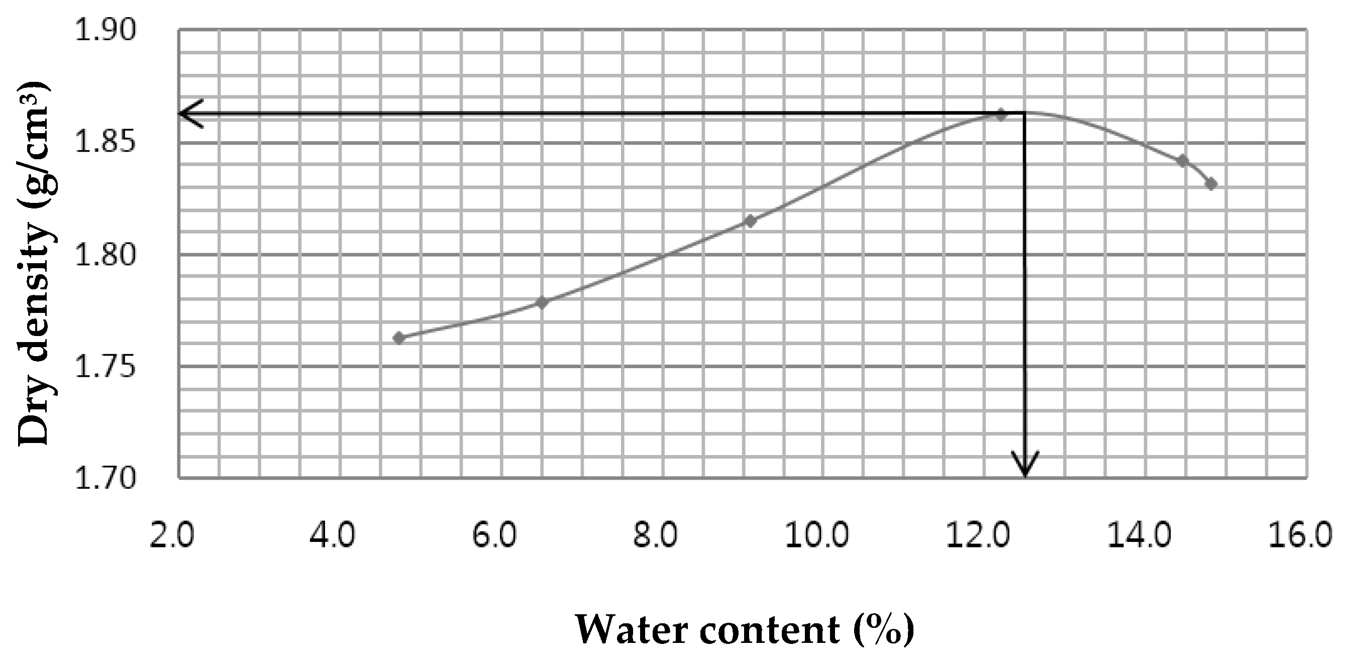
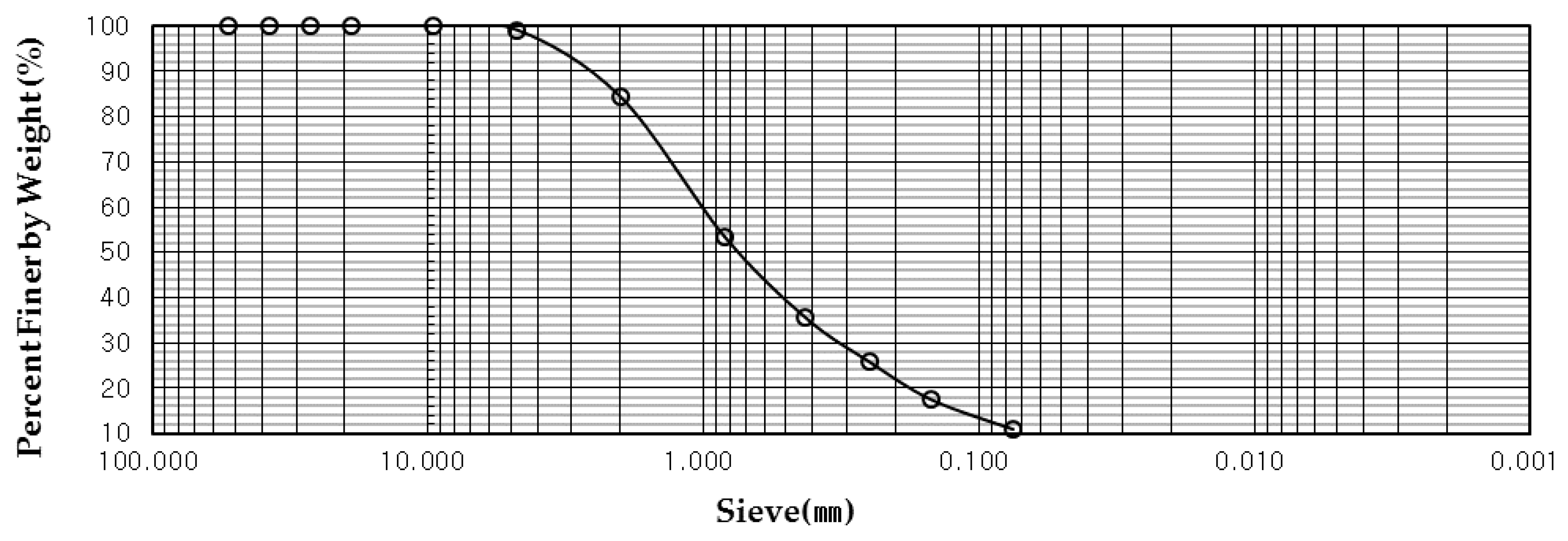
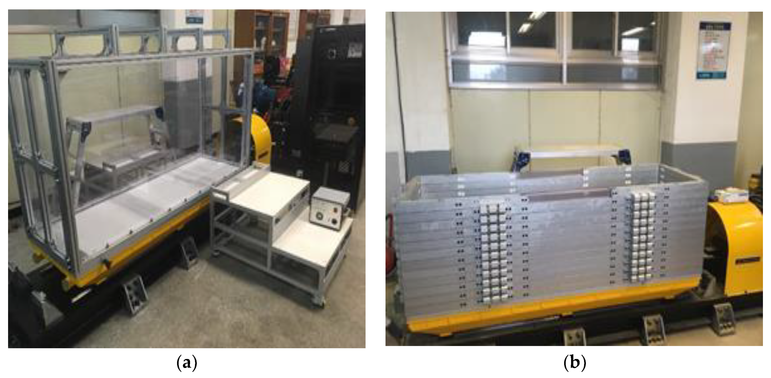
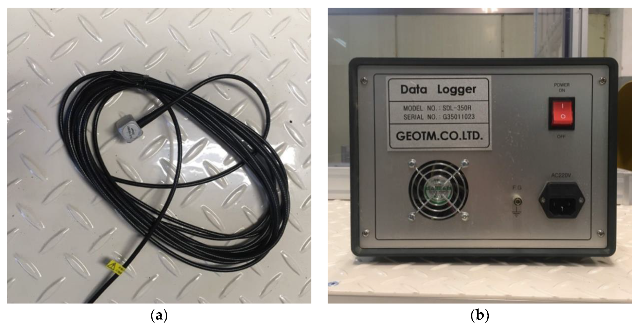
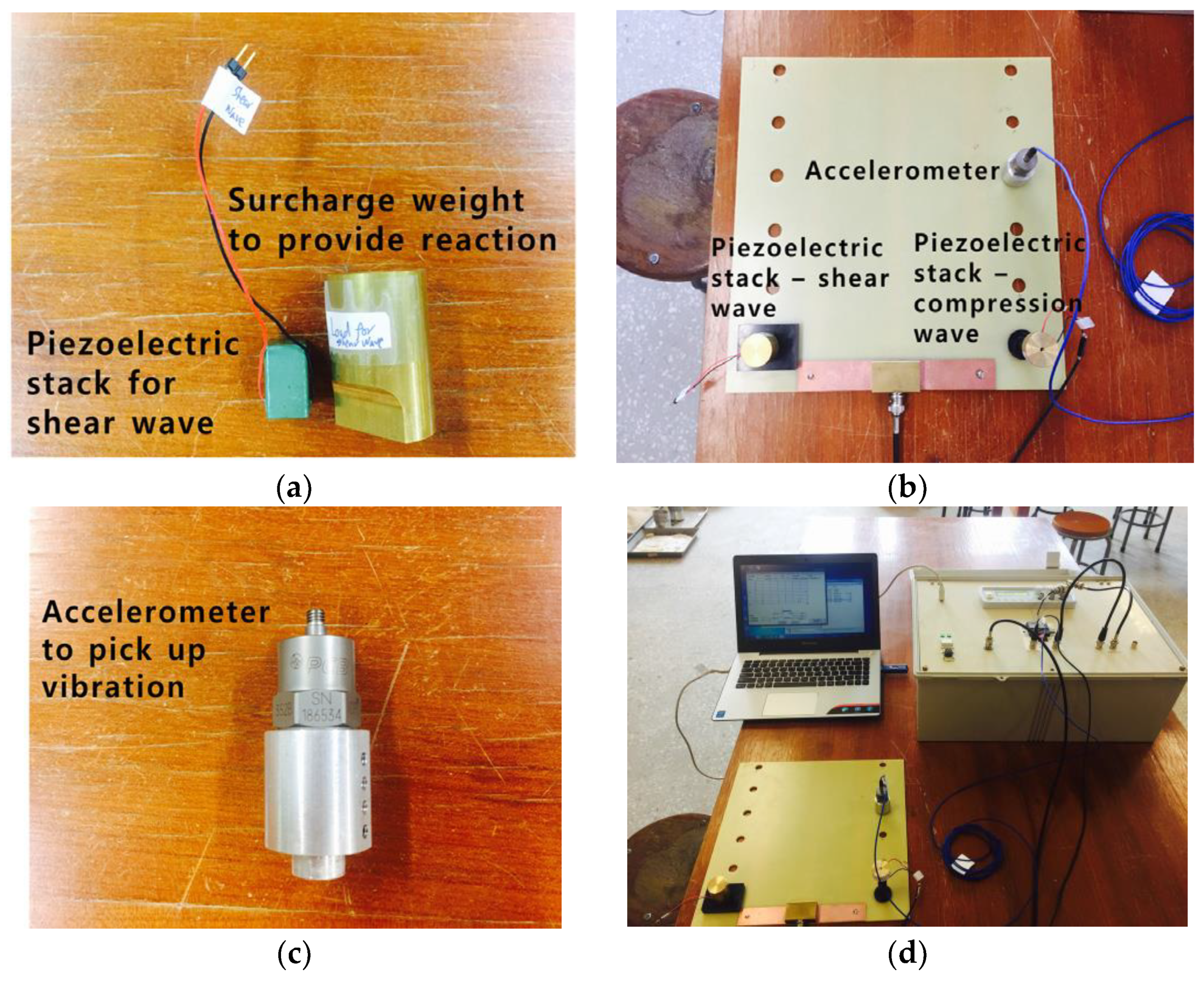
2.1. Soil Used for Creating Ground and Test Equipment

The soil for the scale model test in this study was collected from a construction site in Korea and the cut slope in the construction site, located at Ulju-gun, Ulsan Metropolitan City, the sample representing weathered soil. The physical properties of the soil were analyzed through the specific gravity test, grain–size test, standard Proctor test and relative density test.

The specific gravity was found to be 2.69 and the result of the standard Proctor test is shown in Figure 1. As shown in Figure 1, the maximum dry unit weight was 18.27 kN/m³, and the optimum moisture content was 12.5%.

The relative density test showed that the minimum dry unit weight was 12.43 kN/m³, and the Atterberg limit test showed Non Plastic (NP) for Plastic Index (PI). Figure 2 exhibits the grain–size distribution curve.

The fines content of the soil was 10.8% and the soil was classified as SW-SM according to the Unified Soil Classification System. For the dynamic model test, the specimen was selected for the sample passing through the No. 4 sieve after the physical property tests, and the sample remaining in the No. 4 sieve was about 1%, not much.

Table 1. Physical properties of soil to be tested.

Physical Properties
Gs	No.200 Passing (%)	OMC (%)	PI (%)	USCS	${\mathbf{e}}_{\mathbf{m}\mathbf{a}\mathbf{x}}$	${\mathbf{e}}_{\mathbf{m}\mathbf{i}\mathbf{n}}$	${\mathbf{r}}_{\mathbf{d} \mathbf{m}\mathbf{a}\mathbf{x}} (\mathbf{kN}/{\mathbf{m}}^3)$	${\mathbf{r}}_{\mathbf{d} \mathbf{m}\mathbf{i}\mathbf{n}} (\mathbf{kN}/{\mathbf{m}}^3)$
2.69	10.8	12.5	NP	SW-SM	1.123	0.443	18.27	12.43

illustrates the result of physical property tests.

The 1 g shaking table used in this study moves horizontally in one direction, and the maximum displacement is 200 mm (±100 mm). Figure 3 shows the RB and the flexible soil box used in this study. The RB is similar to the ones that are typically used. The front, sides and back of the boxes are made of clear polyethylene of 10 T in thickness, and the profile for arranging and fixing accelerometers and displacement sensors is fixed on top the soil box. Four drainages, 5 mm in diameter, are provided at the bottom. The walls are integrated as in conventional soil boxes with rigid walls, and sized to be 2000 (L) × 600 (B) × 1000 (H) mm. Since the RB model or walls generally used constrains on the lateral shear motion of ground, it is very difficult to simulate the infinite free field ground completely. The size of LSB was 2000 (L) × 600 (B) × 600 (H) mm and it was made to have the same bottom section as the RB, but some layers in height. Each layer is 45 mm in thickness, the layer spacing is 5 mm to have 12 layers, each of which allows divided lateral behaviors, and the walls are made of aluminum. The natural period of the empty LSB is 0.04–0.05 s.

Figure 4 shows the accelerometer and the data logger used for detecting and measuring data in this test. The same type of the accelerometer that Park [9] used was used in our study. The response acceleration measured in this test was expected not to be faster than 20 m/s² in terms of range, and the assumption was based on the frequency component of response data not being greater than 40 Hz, and the room temperature. Therefore, the selected accelerometer was ARF-20A, which can measure up to 20 m/s². The data logger had 12 channels and was compatible with ARF-20A as a 4 Gage Sensor, and the data collection interval was maximum 0.001.

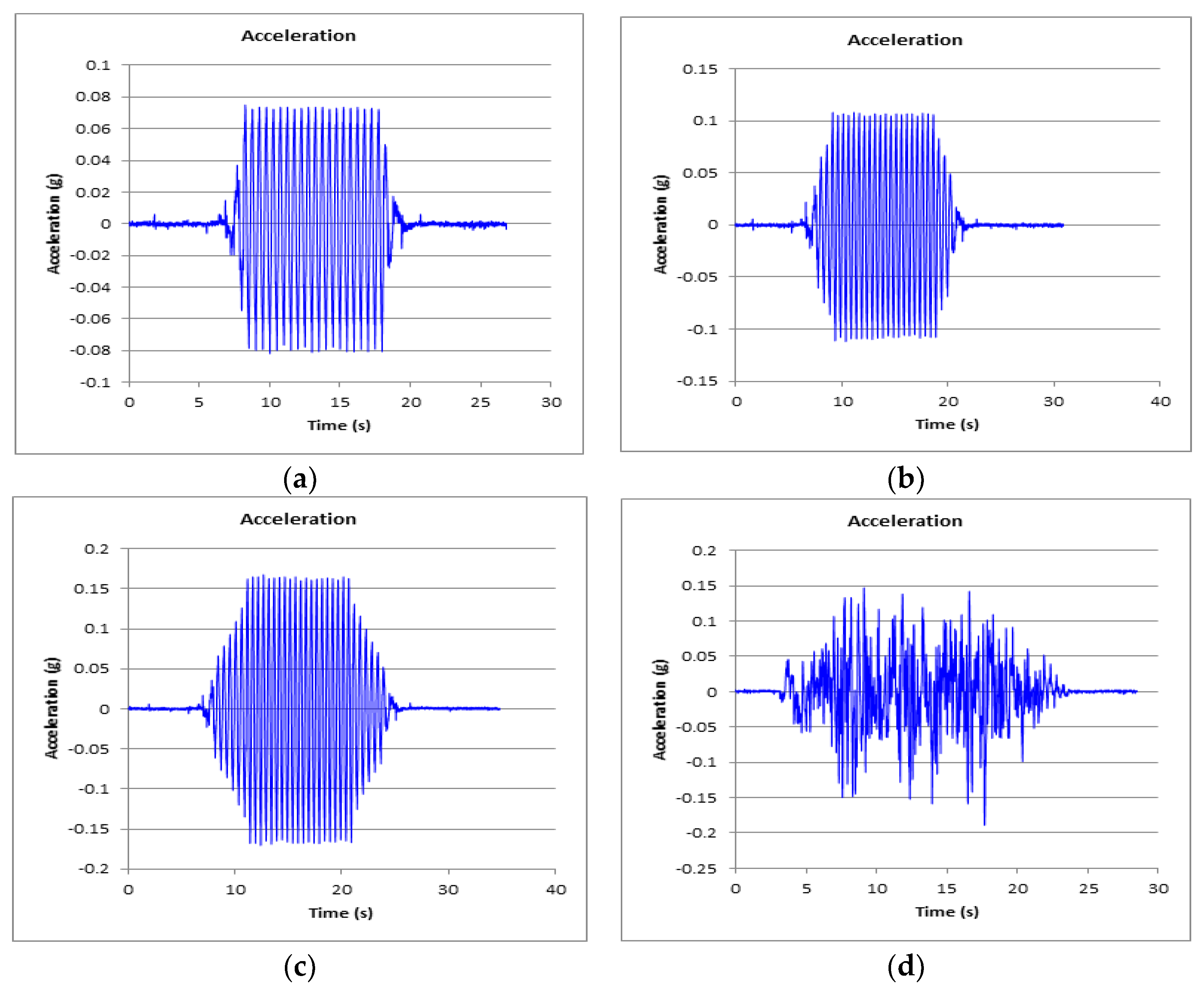
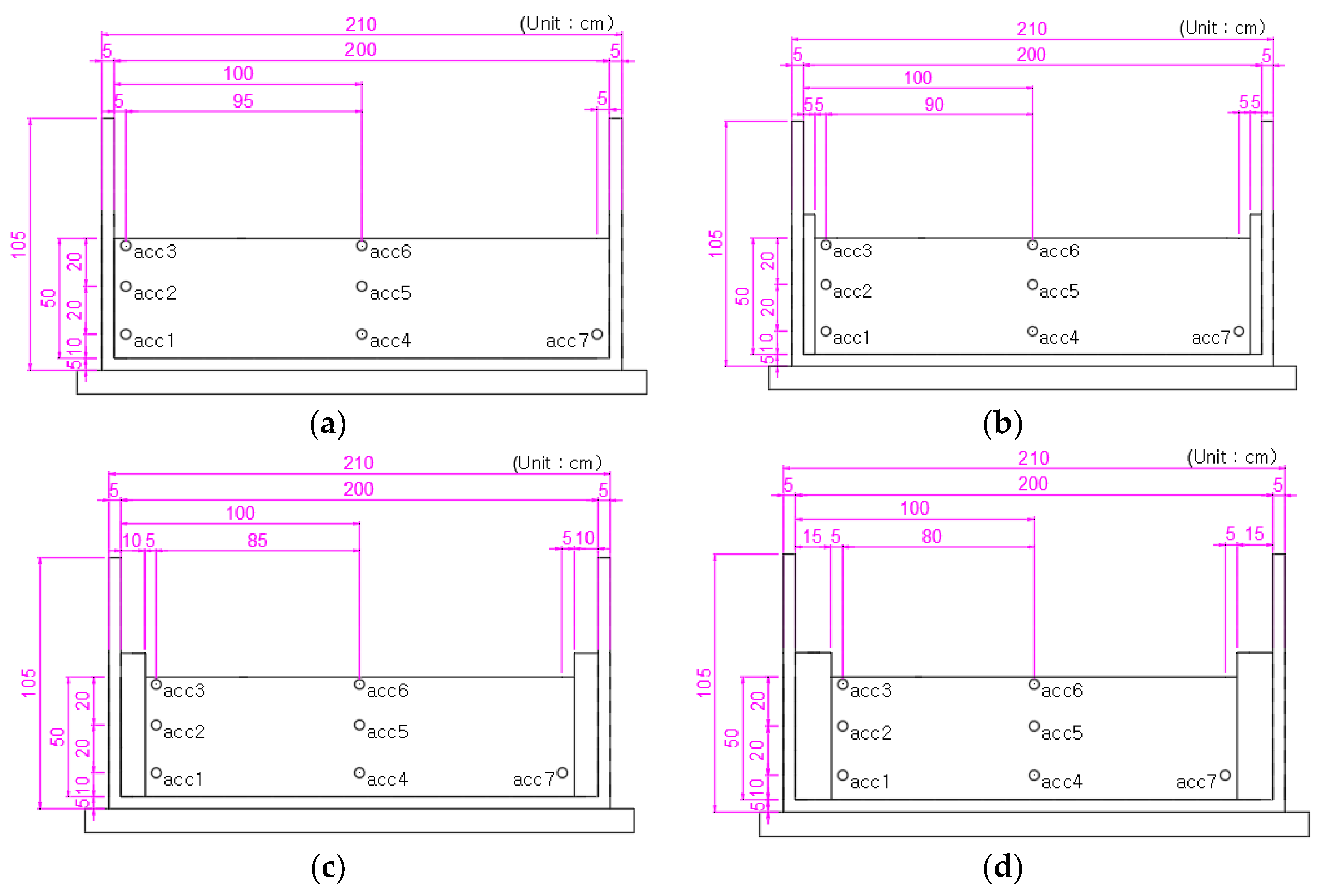
2.2. Configuration of Test Program

The test models were divided to analyze boundary conditions depending on wall conditions of the soil boxes before the test. Five cases were presented depending on the soil boxes to be tested, the slope of ground model (geometric shape), and the presence of sponge on the wall in the direction of vibration. Load input was 3 sine waves (0.07 g, 0.1 g, 0.154 g) and an artificial seismic wave (0.18 g). In other words, 4 types of loads were inputted after setting up 5 cases to conduct the dynamic model test 20 times (

Table 2. Classification of test model and input wave.

Case	Soil Box	Slope	Sponge	Input Wave
1	RB	Flat (Height 50 cm)	–	Sine wave	0.07 g
2			50 mm		0.1 g
3			100 mm		0.154 g
4			150 mm	Artificial earthquake	0.18 g
5	LSB		–

).

Figure 5 shows the waves entered including the sine wave and the artificial seismic wave at different acceleration levels. The sine wave was selected to be 0.07 g, 0.1 g and 0.154 g of 2 Hz. In order to confirm that the effect of the boundary condition changes with the size of the load, we tried to exclude elements other than the load as much as possible. Therefore, a simple long-cycle sine wave, 2 Hz, was selected so that resonance does not occur due to the natural period of the shaking table or box. The 2 Hz sine wave of 0.07 g was selected to examine the effect of boundary conditions, when applying the small enough load and the long-period waveforms without significant amplification, for each height of the scale model to be tested. The artificial seismic wave is the synthetic seismic wave combining the Gyeongju–Pohang earthquakes, using the empirical Green’s function on the basis of the raw data measured in the Kori Nuclear Power Plant. As the artificial seismic wave has different periodic components, high amplification occurs. This is why the artificial seismic wave was selected to evaluate the effects of boundary conditions in the case of high amplification.

Figure 6 shows the locations of measurement by the accelerometer installed in the center of the soil box and the walls therein, which are 10 cm, 30 cm, 50 cm high, respectively, from the bottom. The accelerometers for the model test using the RB of Case 1 and the flexible soil box of Case 5 were installed, as shown in Figure 6a, to analyze acceleration changes at the same locations. Although each ground length is different because of the added sponge in Case 2, Case 3 and Case 4, the center and heights of the ground were the same, as shown in Figure 6b–d. The accelerometer buried in the walls were spaced 5 cm apart from the wall and the sponge. This aims to observe changes of response acceleration amplification between the center and the wall of flat ground occurring depending on boundary conditions of the soil box at the center and the wall, for the same height. All cases were homogeneously constructed with the same compaction and water content using the same soil.

For the model, the relative compaction was 70%; the optimum water content was 12.5%; the void ratio was 1.055; the dry unit weight was 12.79 kN/m³, and the moist unit weight was 14.22 kN/m³. For the RB supported with a sponge, the sponge was attached before creating the ground, and the soil can be compacted by means of lateral pressure while creating the soil where the rigidity of sponge is too low. For selecting the sponge of which the density is not greater than the density of created ground, the selected sponge was 0.49 kN/m³ in density and 15.6 kPa in hardness (resistance to deformation).

Figure 7 shows the shear wave velocity (Vs) measurement equipment in the shear wave velocity test, used to examine the characteristics of the ground model by Song [12]. The shear wave velocity test is a method for calculating Vs by allowing the Piezoelectric stack to generate signals to make the shear wave flow through the ground, and defining the time when the first signal is read as the first arrival time when the accelerometer, separated by a given distance from the creator, catches the signal. To facilitate contact between the soil surface and the Piezoelectric stack, additional weights were made and placed on top. This was to ensure that the vibrations generated by Piezoelectric stacks can be transmitted to the soil well.

3. Analysis of 1 g Shaking Table Test Result

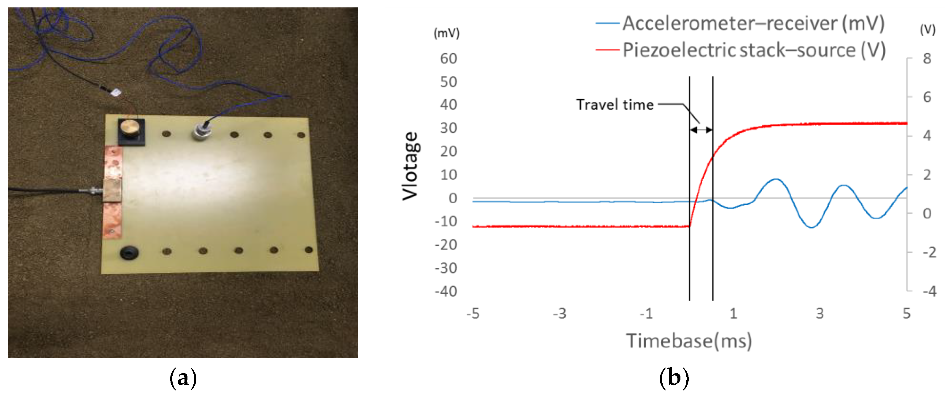
3.1. Shear Wave Speed

The shear wave velocity test measures the first wave arrival time to find the speed with the knowledge of the distance between the Piezoelectric stack and the accelerometer. The shear velocity is measured, as shown in Figure 8a, and the travel time is calculated by the distance between the point at which the input voltage begins and the point at which the output voltage begins, as shown in Figure 8b. The shear wave speed measured in the RB was 101.91 m/s in the shear wave velocity test; in the flexible soil box, it was measured to be 93.59 m/s in the shear wave velocity test.

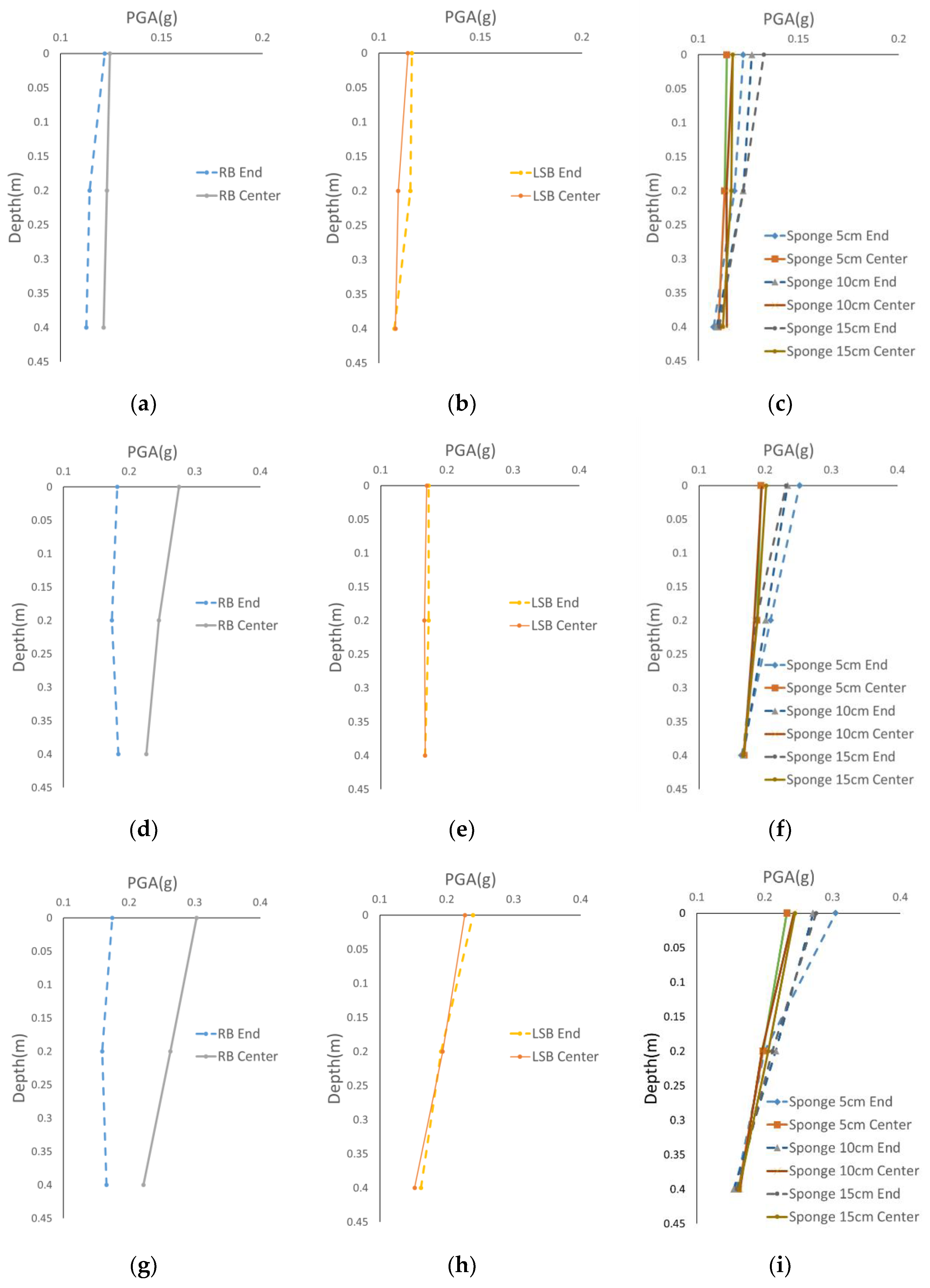
3.2. Analysis of Peak Ground Acceleration

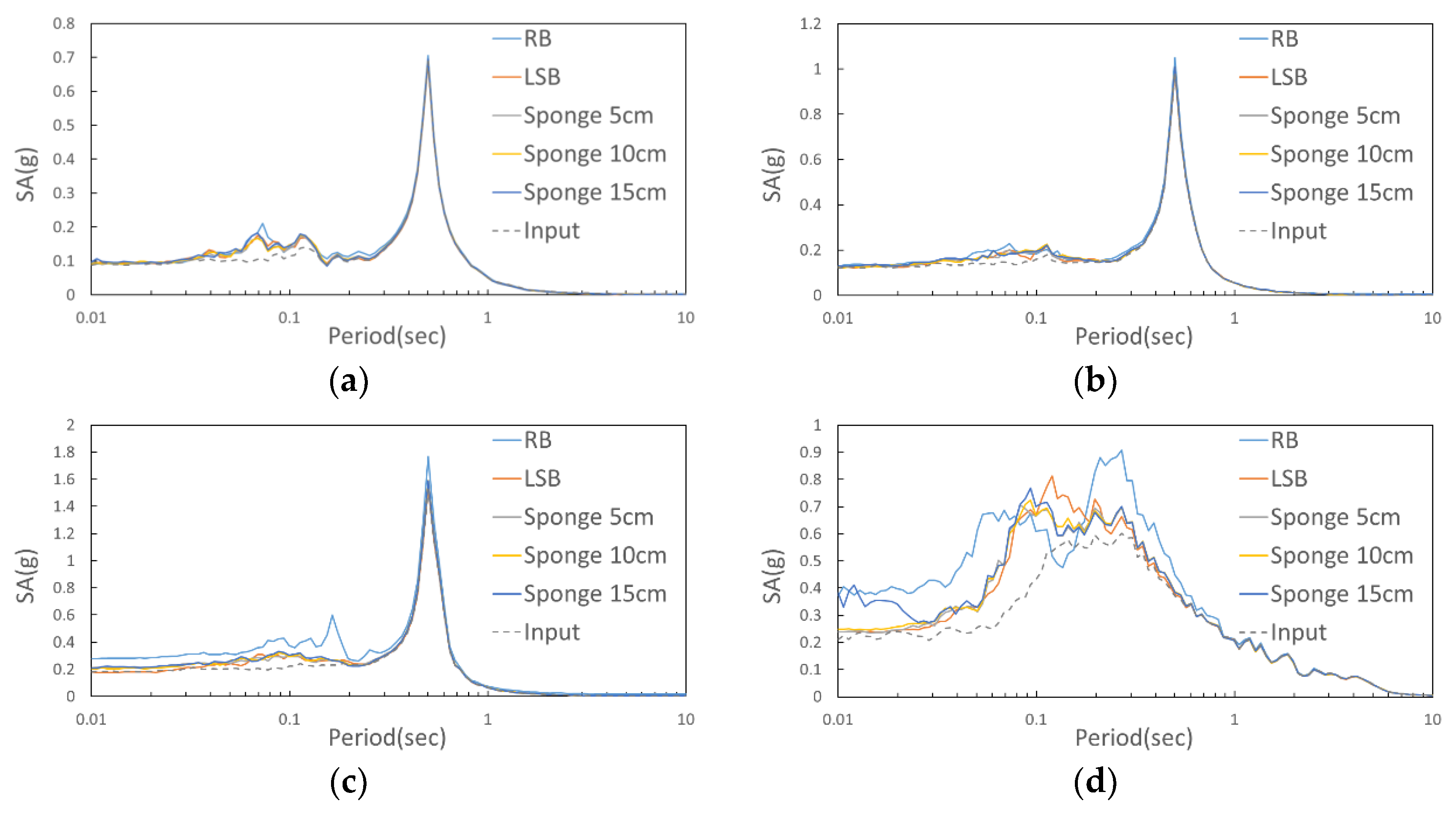
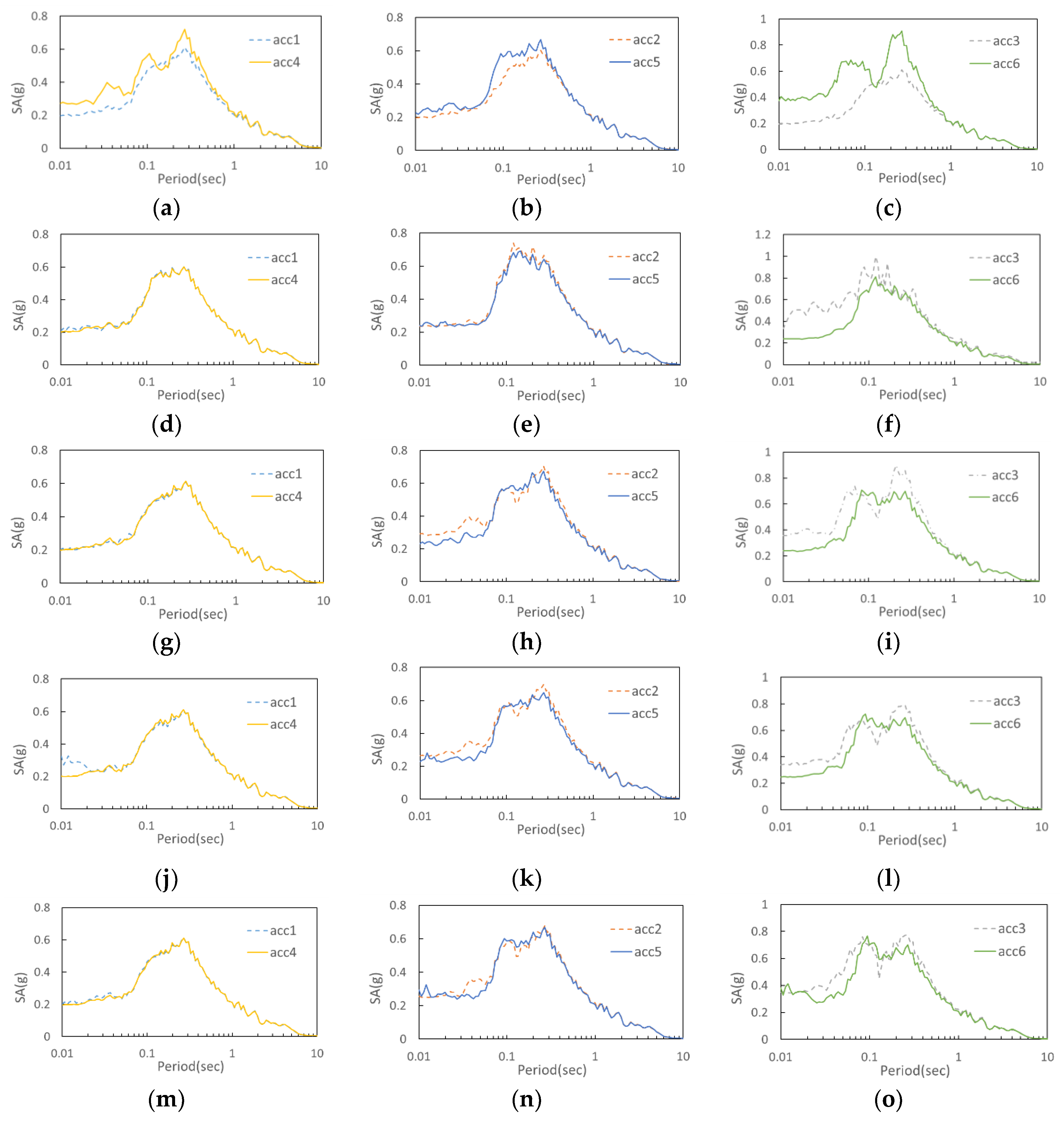
PGA means the maximum acceleration at which the ground moves by means of dynamic load. In this study, the PGA was measured at the same depth in the center and the wall of the soil boxes to analyze acceleration distributions depending on the distance from the center of the model ground to the wall. As the ground acceleration at the same depth in the free field should be the same regardless of the distance, the effect of boundary conditions is evaluated by investigating whether the acceleration in the wall is different from that in the center of the soil box closer to the free field. Since the center acceleration in the soil box is not or little affected by the wave reflection, this acceleration was assumed to be the response acceleration occurring in the free field. The acceleration at the wall was measured from the location 5 cm apart from the wall. The level of bad effect of rigid boundary related to the resonance of the wall was evaluated with the PGA/ response spectrum at the center and end of the RB and the LSB.

Figure 9 shows graphs depicting the peak ground acceleration for each depth of the ground model for various input motions shown in Figure 7. The graphs compare the PGA at the center and the wall in the soil box for each depth of the center, and the wall for each soil box. Almost no amplification was observed from the bottom to the top of the ground model in the wall of the RB, but a significant amplification was observed in the center, implying a great difference between them. Meanwhile, in the flexible soil box, the amplification in the center and the wall was shown to be very similar from the bottom to the top of the ground model. Where a sponge was attached to the rigid wall, greater amplification was observed at the wall than the center, regardless of the thickness of the sponge, and at the center a similar amplification was measured to that of the flexible soil box. In the RB, the lateral boundary was constrained to cause the model ground to have a motion different from the free field, and the reflected wave occurring in the wall caused different stresses, resulting in the excessive amplification in the center. The flexible soil box is considered to simulate the free field behavior of semi-infinite–half-space well to show the amplification factor similar at the same depth in the center and the wall of the soil box. While the sponge attached to the RB contributes to reducing the effect of boundary conditions of the RB so that the center can show similar amplification to the flexible soil box, the wall is affected by the boundary conditions to show different amplification from the center.

3.3. Analysis of SA

Ground response to the dynamic load varies with the natural frequency of the ground and the frequency of seismic vibration. The response spectrum is the maximum response to seismic vibration with different natural frequencies. When acceleration is defined as a response variable, it is called SA (Spectral Acceleration). SA shows the maximum response acceleration given by dynamic load to the vibration meter of different periods. Using this feature, it is possible to examine the amplification occurring in other frequency ranges for the dynamic load used in the actual test.

Figure 10 shows the 5% damped response acceleration spectra measured by the accelerometer (acc6 shown in Figure 5) in the center of the soil box for 2 Hz sine wave of 0.07 g, 0.1 g and 0.154 g, as well as the artificial seismic wave. This aimed to examine the difference of amplification characteristics occurring in the center of each soil box. For 2 Hz of 0.07 g and 0.01 g, Figure 10a,b do not show a great difference between the soil boxes. Since the period of 2 Hz does not match the natural period of the soil box and the ground model, much amplification does not occur. For 2 Hz of 0.154 g, Figure 10c shows that the ground model of the flexible soil box and the soil box with the attached sponge did not react, but much amplification took place on the surface acceleration of the RB. This is due to the quite large magnitude of the earthquake load that caused unnecessary amplification. For 2 H of 0.154 g, Figure 10d shows the surface acceleration spectrum in vibration with artificial seismic waves, in which greater amplification occurs with height, to suggest clearer amplification differences between the soil boxes because the artificial seismic wave has different period components. The flexible soil box and the soil box with the attached sponge show similar amplification, but the soil box with the attached sponge showed slightly greater amplification, and major amplification periods were also similar. In contrast, the RB showed different major amplification periods from the flexible soil box and the soil box with the attached sponge, and showed greater amplification.

Figure 11 shows acceleration spectra in the center and the wall of the soil box at the same depth for the artificial seismic wave shown in Figure 7d. Figure 11a–c show acceleration spectra for the RB with depths. The results show that the center has slightly higher amplification than the wall at the depths of 0.4 m and 0.2 m, and the center of the RB clearly has more amplification on the surface, exhibiting a very different spectrum from the wall. This indicates that that different amplification occurred in the ground model. It appears that the shear wave reflected on the constrained rigid lateral boundary surface had an effect, as great PGA was measured in the center of the RB.

Figure 11d–f show the 5% damped acceleration spectra for each depth of the LSB, showing almost the same spectrum in the center and the wall at the depths of 0.4 m and 0.2 m. In other words, the flexible soil box experienced the same acceleration amplification in the center and the wall, like free field behaviors of a semi-infinite half-space. However, the wall showed greater amplification than the center on the surface. When a dynamic load was used in the flexible soil box for vibration, most layers in the wall showed integrated behaviors with the ground model and simulated the behaviors of the semi-infinite half-space. However, because of no surcharge load, the wall in the top layer was affected significantly by inertia to make a difference from the behaviors of the model. This caused separation and re-contact after separation between the wall in the top layer and the soil, and unnecessary impulsive load was given to the accelerometer in the wall.

Figure 11g–o show the 5% damped acceleration spectra at each depth of the RB with the attached sponge, showing almost the same spectrum in the center and the wall at the depth of 0.4 m like the flexible soil box, and a similar tendency at the depth of 0.2 m. The soil box with the attached sponge showed great amplification in the wall on the surface at the amplification period between 0.2 and 0.3 s, and the wall rather than the center had a high-frequency component at the amplification cycle between 0.05 and 0.08 s, having a spectrum moving toward the left. In other words, although the sponge attached to the RB reduces the effect of boundary conditions to show similar behaviors in the center and the wall in the ground, the boundary effect is not completely addressed on the surface, having more amplification in the wall. It is considered that the difference between the materials of the rigid wall and the sponge, and the natural periods, contribute to the difference in the major amplification periods in the center and the wall.

4. Conclusions

One of the important requirements for performing the 1 g shaking table test or the centrifuge test is to use a soil box that can simulate the free field behavior of the soil as closely as possible. The RB is known to have some boundary problems due to the constraint of the lateral displacement of the model soil. In order to better simulate the model soil subjected to earthquake loadings, two types of soil boxes, the RB and the LSB, were compared for sine waves and artificial seismic waves. This study is focused on comparing PGA and response spectrum for the same soil to evaluate the performance of the RB and LSB, although there are many aspects in practice. Based on the test results, the following conclusions can be drawn:

(1)

For the RB, the amplification of Peak Ground Acceleration and Spectral Acceleration at the center was greater than that of the wall. This implies that the ground model motion is different from free field because the lateral boundary of the RB is constrained, and the reflected wave occurring in the wall generates different stresses to amplify acceleration.

(2)

In contrast, for the LSB, both the Peak Ground Acceleration and the acceleration spectrum are similar at the same depth in the center and the wall of the soil box, respectively. This indicates that the LSB is better than the RB when performing the 1 g shaking table test for understanding the dynamic behavior of soil.

(3)

In order to evaluate the possible reduction in the boundary problems, sponges were attached to the side wall of the RB. Although the major amplification period of the wall and the center on the surface showed a slight difference when a sponge was attached to the RB, the center and the wall in the ground model showed similar behaviors, implying that the use of sponges in the RB may mitigate some boundary effects. However, because the rigidity varies with the types of sponges, the material selected for the test contributes to different effects of reducing boundary conditions, and the sponge thickness between 5 cm and 15 cm did not exhibit a significant impact on the result.

References

1. Kokusho, T.; Iwatate, T. Scaled model tests and numerical analyses on nonlinear dynamic response of soft grounds. Proc. Jpn. Soc. Civ. Eng. 1979, 1979, 57–67. [Google Scholar] [CrossRef] [Green Version]
2. Lamb, T.W.; Whitman, R.V. Soil Mechanics; SI Version; John Wiley & Sons Inc.: New York, NY, USA, 1969. [Google Scholar]
3. Fiegel, G.L. Centrifugal and Analytical Modeling of Soft Soil Sites Subjected to Seismic Shaking; University of California, Davis: Davis, CA, USA, 1995. [Google Scholar]
4. Sundarraj, K.P. Evaluation of Deformation Characteristics of 1-g Model Ground During Shaking Using a Laminar Box. Ph.D. Thesis, University of Tokyo, Tokyo, Japan, 1996. [Google Scholar]
5. Lee, Y.J. Development of Laminar Box Manufacturing Technique for Earthquake Engineering. Master’s Thesis, Seoul National University, Seoul, Korea, 2001. [Google Scholar]
6. Kim, J.M.; Ryu, J.H. Numerical Evaluation on the Model Ground Motion Characteristics of Rigid and Laminar Shear Box Systems. J. Res. Inst. Ind. Tech. 2007, 66, 39–45. [Google Scholar]
7. Kim, J.M.; Ryu, J.H.; Son, S.Y.; Na, H.Y.; Son, J.W. A Comparative Study on Dynamic Behavior of Soil Containers that Have Different Side Boundary Conditions. J. Korean Geotech. Soc. 2011, 27, 107–116. [Google Scholar] [CrossRef]
8. Son, J.W. A Comparative Study on Dynamic Behavior of Soil Containers Having Different Boundary Conditions. Master’s Thesis, Busan National University, Seoul, Korea, 2012. [Google Scholar]
9. Park, S.B. Effect of Installation Angel of Soil Nail on Dynamic Slope Behavior. Ph.D. Thesis, Chungbuk National University, Seoul, Korea, 2015. [Google Scholar]
10. Kim, H.S. Dynamic Behavior of Friction Pile According to Shape of Pile Cap. Master’s Thesis, Chungbuk National University, Seoul, Korea, 2016. [Google Scholar]
11. Bhattacharya, S.; Lombardi, D.; Dihoru, L.; Dietz, M.S.; Crewe, A.J.; Taylor, C.A. Model Container Design for Soil-Structure Interaction Studies. In Role of Seismic Testing Facilities in Performance-Based Earthquake Engineering; Fardis, M.N., Rakicevic, Z.T., Eds.; Springer: Dordrecht, The Netherlands, 2012; pp. 135–158. [Google Scholar]
12. Song, M.W.; Kim, W.M.; Kim, D.H.; Choi, C.Y. Prediction of the Elastic Modulus of Improved Soil Using the Flat TDR System. J. Korean Geotech. Soc. 2016, 15, 77–85. [Google Scholar]
Figure 1. Compaction curve of soil to be tested.
Applsci 10 04642 g001
Figure 2. Grain–size distribution curve of soil to be tested.
Applsci 10 04642 g002
Figure 3. Soil box: (a) RB; (b) LSB.
Applsci 10 04642 g003
Figure 4. Instrumentation: (a) Accelerometer; (b) Data logger.
Applsci 10 04642 g004
Figure 5. Input motion: (a) Sine wave 2 Hz, PGA 0.07 g; (b) Sine wave 2 Hz, PGA 0.1 g; (c) Sine wave 2 Hz, PGA 0.154 g; (d) Artificial seismic wave, PGA 0.18 g.
Applsci 10 04642 g005
Figure 6. Arrangement drawing of accelerometer: (a) Arrangement drawing of Case1, Case 5; (b) Arrangement drawing of Case 2; (c) Arrangement drawing of Case3; (d) Arrangement drawing of Case 4.
Applsci 10 04642 g006
Figure 7. Shear wave velocity measurement: (a) Piezoelectric stack for shear wave and weight; (b) Accelerometer to pick up vibration; (c) Combined component; (d) The whole view of the TDR system. (Song, [12]).
Applsci 10 04642 g007
Figure 8. Shear wave velocity measurement and result: (a) Shear wave velocity measurement; (b) Travel time of elastic wave obtained by using the Piezoelectric stack.
Applsci 10 04642 g008
Figure 9. Peak ground acceleration by input motions: (a) PGA of RB by Sine wave 2 Hz, 0.1 g; (b) PGA of LSB by Sine wave 2 Hz, 0.1 g; (c) PGA of sponge by Sine wave 2 Hz, 0.1 g; (d) PGA of RB by Sine wave 2 Hz, 0.154 g; (e) PGA of LSB by Sine wave 2 Hz, 0.154 g; (f) PGA of sponge by Sine wave 2 Hz, 0.154 g; (g) PGA of RB by Artificial seismic wave; (h) PGA of LSB by Artificial seismic wave; (i) PGA of sponge by Artificial seismic wave.
Applsci 10 04642 g009
Figure 10. Surface acceleration spectrum by input motion: (a) Sine wave 2 Hz, 0.07 g; (b) Sine wave 2 Hz, 0.1 g; (c) Sine wave 2 Hz, 0.154 g; (d) Artificial seismic wave.
Applsci 10 04642 g010
Figure 11. Acceleration spectra by depth: (a) Depth 0.4 m of RB; (b) Depth 0.2 m of RB; (c) Surface of RB; (d) Depth 0.4 m of LSB; (e) Depth 0.2 m of LSB; (f) Surface of LSB; (g) Depth 0.4 m of Sponge 5 cm; (h) Depth 0.2 m of Sponge 5 cm; (i) Surface of Sponge 5 cm; (j) Depth 0.4 m of Sponge 10 cm; (k) Depth 0.2 m of Sponge 10 cm; (l) Surface of Sponge 10 cm; (m) Depth 0.4 m of Sponge 15 cm; (n) Depth 0.2 m of Sponge 15 cm; (o) Surface of sponge 15 cm.
Applsci 10 04642 g011