Abstract
The imaging technique provides an efficient non-intrusive way for studying local sediment transport with a low rate in open-channel flows. It aims to track all sediment trajectories above the background consists of similar particles (i.e., top-view images of the channel). For this area of interest, currently used imaging methods can be summarized as a two-step framework for identifying and matching active bed-load particles. While effective against a simple and clear background, the two-step approach fails to yield accurate and uninterrupted Lagrangian paths for the sediment particles against complex image background consists of similar particles. This study presents a three-step approach to improve the accuracy of the tracking method. The first two steps of this approach based on image subtraction, centroid exaction and Kalman filter entail improvements to those of the classic methods. The third step based on the nearest neighbor algorithm and spline interpolation manage to identify broken chains and connect them to reconstruct uninterrupted Lagrangian paths of the sediment particles. The verification against simulated images and experimental data shows that the improved three-step approach yields more accurate estimation of bed-load kinematics than the classic two-step method.
1. Introduction
Sediment transport in fluvial streams is an important topic in hydraulic and environmental engineering [1,2,3]. Though, it has drawn wide attention for over a century, the physics of bed-load motion at grain scale remains challenging to experimental efforts due to the excessive difficulty in instrumentation in such complex turbulence-particle-bed interaction [4,5,6,7].
In recent years, the image-based sediment particle tracking methods have been proved repeatedly as a powerful quantitative tool for measuring kinematic parameters concerning bed-load transport at the grain scale, including particle velocity, flight length, entrainment/deposition rate, and the transport rate [7,8,9,10,11,12,13,14]. RGB-D sensors can also be used for measuring the surface of dry granular flows [15,16]. Early researchers applied the particle tracking velocimetry (PTV) from the flow field measurement community directly to track particles at grain scale [17]. However, traditional PTV can identify the speed of particles, but not track the particle individual trajectories. The trajectory of sediment particles is the basis for obtaining many important variables in sediment dynamics, such as the number of active particles, particle velocity, length and duration of trajectory, distributions of entrainment, deposition and gliding particles. Most of the currently used particle trajectory tracking methods can be summarized as a two-step framework, i.e., identifies active particles in each image frame in the first step, and matches active particles between successive frames and obtains the Lagrangian paths in the second step [18,19]. In the first step, the consecutive image subtraction and averaged-background subtraction are often used in changing background [19,20,21,22] and static background [23,24], respectively. In the second step, several algorithms have been developed for matching particles such as gray cross-correlation [13,25], and the nearest neighbors minimal-distance method [23,24,26].
The two-step approach behaves effectively and efficiently for sparsely distributed particles measurement against transparent and uniform backgrounds, especially the side-view image or top-view image with a fixed bed [26,27]. However, they usually perform poorly against complex background which usually is top-view image with mobile bed. The example is shown in Figure 1, which is an image from the experiment of bed-load regime with low transport intensity (the detail of the experiment is introduced in Section 4.1). There are three characteristics of this image: (i) moving particles are similar with static particles in shape and size; (ii) particles sparsely entrained and deposited from the bed; (iii) the background will change when particles entrained and deposited. When the channel bed composed of sediment with similar geometrical characteristics, the nearby particles in the background similar in shape may lead to mismatching when tracing the Lagrangian path of a sediment particle. The color points in Figure 1 shows the result of a typical two-step method, which marks the continuous sediment movement paths. The flow direction is from the bottom to the top. However, there are a large number of errors and missing Lagrangian paths in the results of these two-step methods by the naked-eyed verification. For example, some ‘tracklets’ (parts of entire trajectories) like 14#, 21#, 25#,29#, 39#, 56# and 74# (highlighted in white rectangle in Figure 1) are the trajectory of the same sediment particle.
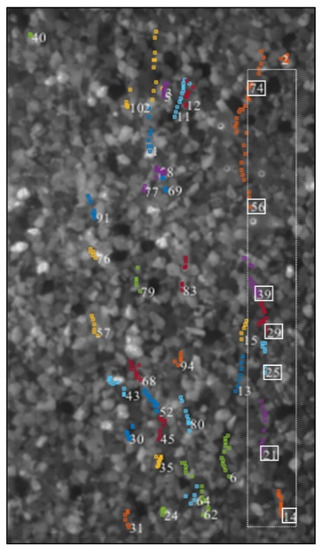
Figure 1.
An example of a two-step method.
Errors and missing Lagrangian paths by the two-step methods will eventually result in the wrong number of active particles and the wrong positions for the entrainment and deposition and then underestimated particle flight length and duration. The number of active particles N is defined as the number of active particles between two consecutive images within the local area. Particle velocity U is the ratio of displacement and sampling interval between two consecutive images. The product of N and U is always used for calculating the transport rate [3]. The positions of particle entrainment and deposition can be easily obtained from the trajectories and they are the key points to resolve the formation mechanism of bed surface morphology. Furthermore, the particle flight length and duration derived from entrainment and deposition positions is relevant to the intermediate ranges of bed-load transport proposed by Nikora et al. (2002) [28]. They can be used for verifying the bed-load transport model. Therefore, the shortcomings of the current two-step method have caused many difficulties in the study of sediment dynamics based on digital image technology. Some methods have been proposed to overcome the shortage of two-step methods. Heyman et al. (2016) [23] used the Jonker-Volgenant algorithm [29] to reconstruct the whole trajectories which is efficient in associating “one-to-one” relationship. However, it is difficult to decide whether the ‘tracklet’ is a broken or a complete one.
This paper reports the development of an improved method to achieve effective and efficient measurement of individual bed-load particles over the mobile bed. The global connection finds and fixes broken chains to reconstruct uninterrupted Lagrangian paths of the sediment particles. The effectiveness of the new method is tested against both artificial and real bed-load transport images. Section 2 presents the improved three-step algorithm step-by-step; Section 3 is a comparative assessment of the algorithm for a set of artificial images where the parameters are known and Section 4 assesses the algorithm for a set of images from a flume experiment.
2. Algorithm
The algorithm includes three steps. In the first step, we preprocess the raw images through a top-hat transformation and image equalization and identify the moving particles by subtracting the previous image from the next image. In the second step, a prediction-confirmation approach is used for accurate identifying the centroids of moving particles. Then the moving particles are matched between two successive images by the cross-correlation coefficient and Kalman filter. In the third step, the nearest neighbor (NN) algorithm and spline interpolation is used for reconnecting and repairing the broken chains. The grayscale image was used for displaying the results of every step. Colored particles should easier be tracked. However, colored images will cost more storage space when captured in high frequency and long duration. This algorithm can deal with not only grayscale image, but also the colored image with more accuracy. Furthermore, this algorithm is suitable for 2D image of bed load transport in rolling and saltation. The particle deformation due to rolling and saltation has been considered and processed.
2.1. First Step: Pre-Processing and Subtraction of Images
Pre-processing of raw images is common practice in imaging technique. A typical raw image of bed-load transport against complex background in open-channel flow is shown in Figure 2a. To facilitate particle identification, the raw image needs to be pre-processed, commonly through a top-hat transformation (to eliminate background non-uniformity) and image equalization (to widen gray level). The effect of such pre-processing enhancement is exemplified in Figure 2b.
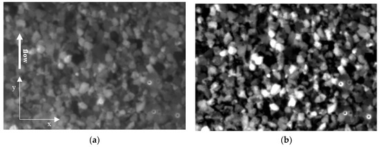
Figure 2.
(a) Raw image and (b) pre-processed image.
Image subtraction between two successive images offers an efficient and effective way to identify moving particles leading to a noticeable change in grayscale [22]. For a moving particle, the subtraction process leaves a pair of patches with relative high value. For the background, the subtraction produces zero patches. Therefore, the images are greatly simplified by subtraction. The unmoving background is removed so that the pixels corresponding active particles are isolated.
2.2. Second Step: Particle Identification and Matching
The image subtraction procedure is the foundation of determining the position of active particles. If the two patches of a moving particle are entirely separate, which is common in low-frequency measurement on a simple and transparent background, it is easy to obtain the position and size of a particle based on image binarization (Figure 3a). The high-frequency measurement will lead to the overlap of two patches (shown in Figure 3b). Direct binarization of the subtracted image entails bias errors for determining particle position, diameter and the displacement between two images (Figure 3b).
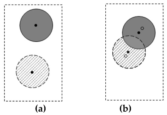
Figure 3.
Sketch of moving particles in two successive frames with (a) low frequency, and (b) high frequency. The dashed and solid circles represent particles in the first and second frames, respectively. The solid round represents a real particle center, and the circle is the particle centroid based on the subtraction procedure.
To solve the overlapping induced problem, we propose a prediction-confirmation approach as follows. First, image-subtraction between image P1 and P2 and subsequent binarization of the subtracted image (P3) yields two centroids in two frames for one active particle, as shown in Figure 4a–c, respectively. These two centroids shown in Figure 4c represent real particle centers in the classic two-step methods. However, they act only as a reference prediction in this method. Second, all the particles within a distance of 1.5 times particle diameter to the centroid recognized in the first image are identified, and their centers can be obtained by direct binarization of P1 shown as blue rounds in Figure 4a,b. The red square in Figure 4a,b represents the searching area of identifying the centroids. The searching distance is determined by frequency and particle shape, which should be slightly larger than the possible maximum distance between two images. As particles cannot move over 1 diameter based on the experimental condition in this paper, the distance should be set as 1 diameter. Moreover, considering irregular shape, 1 diameter may not cover one whole particle, then 1.5 times diameter is selected. The nearest position is then determined to be the real centroid of an active particle. The blue rounds are the re-recognized centroid of the particle, which are closer to the real center of particles.
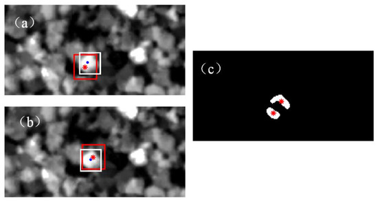
Figure 4.
(a) Moving particle in the original position; (b) moving particle in current position; (c) binarization after two image subtraction. Red star and blue points represent particle center determined through classic subtraction procedure and the current prediction-confirmation procedure, respectively. The red square and white square is the searching area for re-recognizing the centroid and diagnostic window.
Once the information of position and size of moving particles are available in each frame, these particles can be matched in consecutive images through Kalman filter. Specific steps are as follows.
- (1)
- Calculation of the cross-correlation coefficients Cv.
The diagnostic windows, W1 in the first frame and W2 in the second frame, are identical in size, equal to the major axis of the particle(white square in Figure 4). The accurate centroid makes sure that the diagnostic window includes the most particle information and little background gray value. It improves the accuracy of the cross-correlation. W1 is centered around (x1, y1), and W2 is centered around the variates (x2, y2) where
in which dx and dy represent variable distances from the center of (x1, y1) in spanwise and streamwise directions, respectively. By varying the center position, a series of W2 can be obtained and the corresponding gray correlation coefficients Cv between W1 and W2 are calculated. The maximum values of dx and dy are determined by the maximum distance of moving particles between two successive images in two directions, written as aD and bD separately. The factors a and b depend on frequency f, camera resolution R, particle velocity U and, particle diameter D. As the average particle displacement in streamwise is restricted to less than one particle diameter, i.e., (U/f)R < 1D, then a = 1. The spanwise velocity is almost zero, and the maximum distance in spanwise is less than 3D, i.e., b = 3, as shown in Figure 5. Note that the values of a and b can be set to other values, and a = 1 and b = 3 achieves satisfactory accuracy and efficiency in this paper.
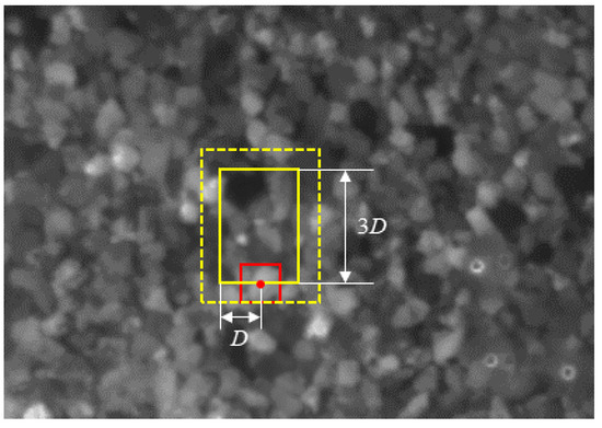
Figure 5.
The diagnostic window (red square) and searching area (yellow square).
- (2)
- Determination of particle position.
The peaks of the correlation coefficient Cv, indicate maximum similarity between the two diagnostic windows (Figure 6a). Thus, the displacement can be determined based on the peaks of Cv. When two or more peaks appear (due to similarity among particles or particle deformation), an additional criterion is required for determining the right one. A combination of the commonly used maximum-value method (which considers the shape and color of active particles) and the Kalman filter (which takes shape and motion parameter of active particles into account) is used in the present study. As shown in Figure 6b,c, we calculated the correlation coefficient of one moving particle between two images within the range of yellow square. Figure 6a shows the contour map of correlation coefficient with two peaks due to particle similarity. Due to particle deformation, the position of the maximum peak is not the correct current position. After the Kalman filter, the corrected current position was closer to the true which marked as blue circle in Figure 6.
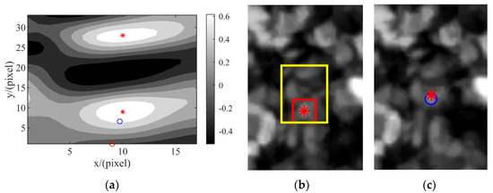
Figure 6.
(a) Contour map of correlation coefficients; (b) moving particle at the first image; (c) moving particle at the second image. The peaks, initial position, and predicted position are represented by red stars, red circle, and blue circle, respectively. Red square and yellow square represents the diagnostic window and searching area, respectively.
The model of particle movement follows approximately a linear dynamic system for which the Kalman filter can be used to predict its behavior. As particles move continually between two successive images, the distance between the current image pair should be related to the previous image pair. The linear Kalman filter estimates the current state at time k based on the state at (k − 1) as follows:
where X(k | k − 1) and Y(k | k − 1) are predictions of x and y-coordinate at time k, respectively, X(k − 1|k − 1) and Y(k − 1|k − 1) are optimal results at time (k − 1), u and v are instantaneous velocity components in y and x-axis, respectively, α(k − 1) is acceleration at time (k − 1), Δt is time interval, and wk1 and wk2 are process noises which follow Gaussian distribution with zero mean. Based on particle shape and gray level, the maximum peak to the prediction is determined to be the position of the measured value, Xm(k) (Figure 6). Bilinear interpolation is then applied to achieve subpixel precision [30].
Note that X(k | k − 1) is determined by particle velocity, acceleration and position in the previous frame, the change in velocity and acceleration will inevitably induce errors. There is an error between Xm(k) and real position because of the similarity between target and background particles. It is recommended that the optimal Kalman gain Kg(k) is applied to contain errors. In the x-direction, for instance, one gets
in which the weight Kg(k) is determined by the covariance P of X(k | k − 1) and Xm(k) as follows,
where R is the measurement error covariance which remains unchanged and P(k | k − 1) is the covariance of the X(k | k − 1) updated by
in which Q is the covariance of process noise (constant), and P(k | k) is the covariance of X(k | k).
The values of Q, R and P (1|1) need to be determined to implement the entire process. The details of determining Q and R can be found in the literature [31]. In brief, R can be determined by some off-line sample measurements and Q is less deterministic. If the measurement is more reliable than the prediction process, Q should be greater than R, and vice versa. The value of P(1|1) can be determined by random, and when it is closer to Q and R, the series of Kg is more stable. In this paper, Q, R and P(1|1) were set as 3, 2 and 3, respectively. Q is set greater than R, which means that measurement value is considered more reliable in our case. The Kg stabilizes quickly and remains constant as 0.69 based on the settings.
As the value of Kg (1) cannot be obtained directly from Equation (5), the maximum peak is chosen to represent the real position in the first image pair.
Repeating the proceeding steps through the entire image series until the last frame yields all the information of moving particles in each frame, including initial positions, displacement, and diameter.
2.3. Third Step: Global Connection
Based on the position and displacement of moving particles, it is easy to track them frame by frame to form a “smooth chain” for each moving particle. However, due to some imperfections such as the influence of moving bubbles and particle deformation due to rolling, the particle identification and matching procedure may fail, and as a result one complete chain may be falsely recognized as two or more sub-chains. These incomplete, sub-chains should be identified and connected; otherwise the flight time and flight length of a moving particle will be underestimated. Heyman et al. (2016) [23] have taken the global connection into account using Jonker-Volgenant algorithm [29]. The Jonker–Volgenant algorithm is more efficient in associating “one-to-one” relationship. However, it is difficult to decide whether the ‘tracklet’ is a broken or a complete one. In our experimental condition, particles move intermittently which means some ‘tracklets’ do not need to be associated. Commonly, a new chain entrained nearby a deposition chain. The Jonker-Volgenant algorithm may mismatching deposition ‘tracklet’ with a new entrained one. Hence, the global connection in this paper is more efficient which includes a pre-judgment of ‘tracklet’, associating broken chains with the NN algorithm and repairing the missing frames.
A complete smooth chain typically exhibits minimal displacement at both ends. A broken chain, on the other hand, generally shows considerable displacement at either end. In the present study, most particles cannot move over one diameter between two consecutive frames. Hence, the criterion to determine complete or broken chain was set as one diameter.
The broken chain also results in “artificial deposition” of a chain and entrainment of a “new” chain nearby in the next frames. Before reconnected broken chains by the NN algorithm, two threshold values in space and time should be set. When a “new” chain appears in the range of the average flight length L (the distance of one flight from entrainment to deposition) during the average flight time T (the duration of one flight), the nearest “new” chain and the present broken chain could be reconnected. Based on these characteristics, all the chains are checked, and the broken ones are connected through spline interpolation. Some short chains, usually fewer than one diameter, are identified as false chains and are directly deleted. The average flight time and flight length can be estimated by the empirical relationship published in the literature, e.g., Lajeunesse et al. (2010) [11]. The proper frequency of this approach was discussed in the literature, e.g., Miao et al. (2018) [32]. The higher limit of frequency should be specified to allow an active bed-load particle to move a “discernable” distance, preferably larger than a few pixels. Based on experience, the higher limit can be set as a product of particle velocity and image resolution. The low frequency may lead to mismatching of moving particles. As recommended by Miao et al. (2018) [32], the lower limit of frequency is diverse of a tenth of flight duration.
After above three procedures to reconnect broken chains, most “artificial depositions” can be reduced. However, some broken chains cannot be reconnected well. When a moving particle collides with the bed, the displacement between two successive images is often smaller than one diameter during this collision. Then if the particle was lost in the first two-step, this trajectory cannot be recognized as a broken chain. Hence, the collision of particles with bed cannot introduce new errors on this approach.
Figure 7 shows the flow chart of the new algorithm, comprised of image pre-processing, image subtraction, image binarization, particle tracking, and global connection. The details of the flow chart are described above.
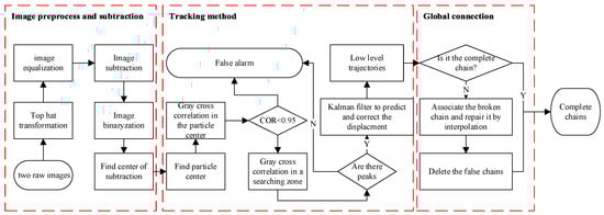
Figure 7.
Flowchart of the new method.
3. Validation by the Simulated Case
The effectiveness of the new approach was tested and verified against simulated images corresponding to an artificially designed bed-load movement pattern of which all the kinematic parameters are fixed and known in advance.
3.1. Images Design
Designing the images involves two key considerations. First, the simulated cases need to be comparable to typical real bed-load movement in common open-channel flow experiments in terms of particle characteristics (size, shape and color), bed configurations, and motion kinematics (entrainment, displacement, speed, etc). Second, the simulated cases cover a relatively broad range in the displacement between two successive images, thus revealing the influence of the measurement.
The image is 250 × 250 pixel2 in size, and there are 8 × 8 particles in length, width evenly distributed across one image as shown in Figure 8a. There are 500 image series with the same particle distribution. The particle, irregular in shape, is designed by superimposing two or three smaller circles (3–5 pixels in diameter) onto a bigger circular particle (11–16 pixels in diameter), as illustrated in Figure 8b. There are 12–15 pixels between the centers of the bigger and smaller circle. Moreover, the combined irregular particle has an average equivalent diameter Ds = 30 pixels. The lowercase represents instant value, and uppercase represents average value in this study.
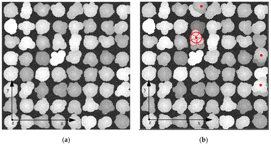
Figure 8.
Two consecutive simulated images, (a) first simulated image, (b) second simulated image. The red points represent the active particles. The solid red circle and dotted red circles mean the combination of one particle.
Particle motion is simplified into an entrainment-flight-deposition pattern. The number of entrained particles follow a negative binomial distribution, as suggested by Ancey (2010) [33] and entrained randomly over the image. Based on this, we set the total number of active particles between two images to be Ns = 590 ± 30. If a particle is entrained, particle placed on its position in the next image will appear instantly. The flight of a particle across two successive images is characterized by time duration and traveling displacement. To investigate the influence of measurement frequency, we set the duration to be constant at one second and used a series of velocities, thus varying the displacement of a moving particle between two successive images. This processing means is equivalent to varying the sampling frequency in a measurement of bed-load motion at a fixed velocity.
Four cases were considered in terms of streamwise velocity, i.e., Us = 0.25Ds, 0.5Ds, 0.75Ds and Ds in a time interval, as shown in Table 1. Note that the velocity is equal to displacement in pixel as the time interval is set to be 1 s. The spanwise velocities vs. in a time interval is set to follow normal distribution N(0, Us/5). The flight length and time are set to be Ls = 5Us and Ts = 5 s, respectively. Note that the range of Ls is broad enough to cover commonly encountered cases in open-channel flow [11].

Table 1.
Summarizes the major parameters of the simulated images.
3.2. Results
Both the classic two-step and the new three-step methods were used to process the simulated images and to quantify the designed bed-load motion pattern. Image processing parameters were kept the same in the two methods. If a particle moves out of the image, its information is not included in the final statistics.
For each case, the 500-frame image series were processed, and thereafter statistical samples were established for calculating various instant parameters including the number of active particles between two images n, particle velocity in the streamwise direction u, particle velocity in spanwise direction v, flight length l, and flight time t. The corresponding capital letters represent the mean value of parameters.
The true values of the number of active particles, streamwise velocity, flight length and flight time are nonzero. Hence, the relative error (mean and standard deviation) of the average value was used as an indicator to compare the performance of the two methods. For instance, the mean relative error in the number of active particles is defined to be
in which, N and Ns represent the mean measured and the real number of active particles in one pair of images, respectively. The relative error in streamwise velocity, flight length and flight time is similarly defined, denoted to be εU, εL and εT, respectively.
The mean and standard deviation of the relative error provides a direct measure of the performance of the two methods. Positive and negative values of the mean value εN indicate overestimation and underestimation of the real situation, respectively. The standard deviation of relative errors represents the dispersion degree of measured parameters. The results are shown in Figure 9. The blue point and red triangle represent relative error by the present method and classic method, respectively.
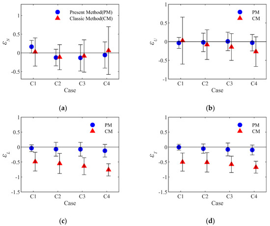
Figure 9.
The mean and standard deviation relative error of N, U, L and T, shown in (a–d) in separate. PM and CM indicated as blue point and red triangle which represent present and classic methods, respectively. The error bars are the standard deviation of relative error.
As shown in Figure 9, the measured values of all parameters by the present method are close to real value with the mean value of relative errors from −12% to 16%. The mean value of εN and εU by the classic method is from −26% to 6% within acceptable range, but slightly more than those by the present method. However, the absolute value of εL and εT are very large, even greater than 50%, which means the flight length and time are significantly underestimated by the classic method. The standard deviation (error bars are shown in Figure 9) of εN, εU, εL and εT by the present method are smaller than those by classic method, which indicates that the present method is more stable and reliable.
Meanwhile, the absolute mean values of εL, εT and εU increase with increased Us by classic method, as shown in Figure 9b–d. However, there is no obvious tendency of εN with Us by classic method, as shown in Figure 9a. These phenomena show that the classic method is more sensitive to article distance between two images, i.e., particle velocity and sampling frequency. The present method performs well in all cases.
For the number of active particles and spanwise velocity, the probability density distributions are set as negative binomial distribution and Gaussian distribution in separate. Therefore, the PDFs of the true and measured value can be used for testing errors.
As shown in Figure 10 and Figure 11, the gray bar and the black line represent the presupposed true value and the fitted PDF of true value, respectively. The red and blue lines represent the fitted PDF of measuring value by the classic and present method in separate. For the number of active particles in Figure 10, two methods yield similar results, consistent with fitted PDF of true value. The results in both Figure 9a and Figure 10 support the effectiveness of the classic method and present method in capturing the number of active particles. However, the present method performs better than the classic method for spanwise velocities, as shown in Figure 11.
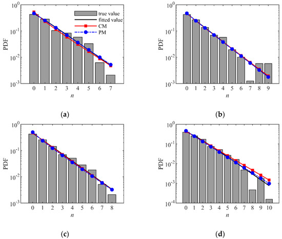
Figure 10.
The probability density distribution of number of active particles in (a) C1, (b) C2, (c) C3 and (d) C4.
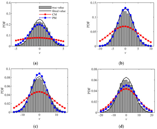
Figure 11.
The probability density distribution of spanwise velocity in (a) C1, (b) C2, (c) C3 and (d) C4.
To summarize, the present method performs well in reporting all parameters with different conditions. The problems caused by frequency and complex background are resolved by the present method.
4. Application in Channel Experiment
4.1. Experimental Setup
Images of bed-load transport were obtained from experiments in open-channel flow. Figure 12 shows the sketch of the experimental setup. The channel is 11 m long, 0.25 m wide, and 0.25 m high. The channel bed slope can be adjusted from 0% to 1.5%. Comb and tailgate are installed in the inlet and outlet of the channel, respectively, to stabilize the flow and water level. Six ultrasonic gauges are used to monitor the water level (with accuracy of 0.1%). Water discharge is measured by the electromagnetic flowmeter (with accuracy of 0.1%). Uniform natural quartz sands were used as bed-load with median diameter of 2.25 × 10⁻³ m and density of ρs = 2650 kg∙m−3. The channel bed was paved with a layer of sand (2.25 × 10⁻² m) before experimenting.
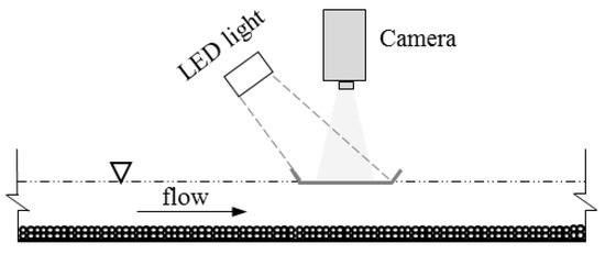
Figure 12.
Sketch of the experimental setup.
A high-speed camera, IDT Y7-S3, with a 50 mm/1.4f lens was mounted above the flow to capture images of sediment motion. The camera has a maximum resolution of 1920 × 1080 pixels and maximum framing frequency of 12, 300 fps. A LED light was used to illuminate the measurement region. A plexiglass sheet was placed on the water surface to eliminate oscillations, similar to procedures used in the literature [7,11,34,35]. Before conducting the experiments, measurements were made to examine the vertical velocity profiles with and without the plexiglass sheet. The results showed that in our experimental condition, the sheet exerts a negligible influence on the velocity profile near the bed. As the bed-load move in the near-bed region, it was regarded that the influence of the sheet on bed-load transport is negligible.
The flume slope J was set to be 2.5‰, water discharge Q was 21.74 m3/h, and the water depth H is 5.33 × 10⁻² m. Hence, the average flow velocity Uf = Q/(HB) was equal to 0.45 m/s, where B is channel width. These hydraulic conditions can ensure that there were particles entrained from the bed and the flow is subcritical. The friction velocity u* = (gHJ)0.5 was 0.036 m/s where g is gravity acceleration equal to 9.81 m/s2. Shields number Θ = u*2/(RgD) was 0.036 which is equal to critical Shields number Θc = 0.036 [13], and where R is sediment relative density equal to 1.65. The Froude number Fr = Uf/(gH) was 0.86. Considering the computational efficiency and water conditions, we set the frequency, image size and total frames as 250 fps, 500 × 864 pixel2 and 60,000 frames, respectively. The choices of these parameters are based on previous experience [32,36]. The resolution of the image was 94.3 pixel/cm, allowing one sediment grain to occupy about 21 × 21 pixel2.
4.2. Results
The images were processed, and the result of 180 frames is shown in Figure 13. Comparison is made among the results from the classic method without Kalman filter (Figure 1), the present method without the third step (Figure 13a), and the current three-step method (Figure 13b). Note that the trajectories are identified and plotted in different colors with number label. The difference between Figure 1 and Figure 13a is clear, i.e., more complete trajectories were identified in Figure 13a. However, some broken chains are still easily spotted in Figure 13a, e.g., 21# and 30#, 76# and 90#, to cite a few. After these broken chains being connected and repaired by spline interpolation, and removing the false chain the final result is shown in Figure 13b. A video was made to illustrate the process of particle tracking (attached to the paper).
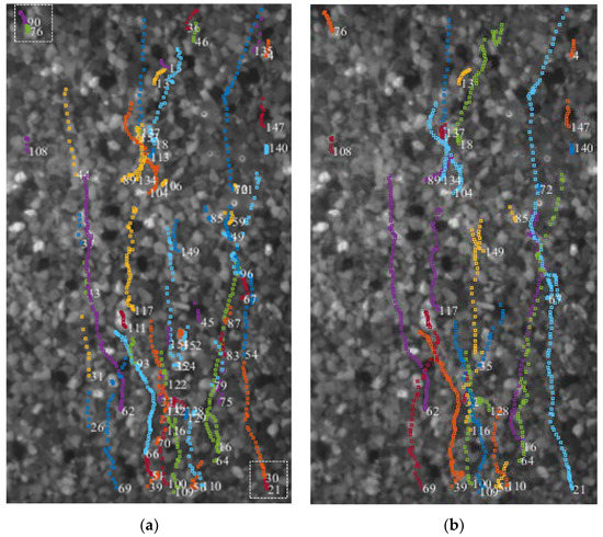
Figure 13.
Particle tracking results by (a) new method without the third step; (b) new method; The different colors represent different trajectories.
After manual checking of the method based on 180 frames, a total number of 60,000 frames were processed for quantitative comparison of bed-load transport parameters between the classic and the present method. The average values are listed in Table 2. The most important parameters in bed-load transport are included, such as the number of moving particles in each frame, N, velocity along the flow direction, U, length of trajectories, L, and duration of trajectories, T.
Table 2.
Results of different algorithms.
It is seen from Table 2 that a significant difference occurs in N, U, L and T. The differences in U, L and T between two methods are similar with results in Section 3.2. The difference of N in the true image between two methods is much larger than that in the simulated image. The differences may be due to smaller pixels and more complex conditions like bubbles and particle deformation in the true image. It is worth to mention that the length of trajectories L is about 8 particle diameters which seems too small to present particle jump length. When a moving particle rest at bed throughout trajectories (0.16 s in Table 2), it was recognized as an independent trajectory. In this paper, it aims to obtain the number of active particles, velocity, the entrained particle and deposited particle in the sampling area. The true particle jump length and duration should be measured with different criteria of reconnecting the “artificial depositions” and larger sampling area.
Based on the present method, it is possible to classify an active particle (showing displacement) into being entrained (from static to motion), deposited (from motion to static), or gliding (in motion) during consecutive images. The number of active particles equal to the sum of number of three kinds of motion state. We statistic the number of entrained, deposited and gliding particles in space based on the time-series image and normalized them by the maximum number of moving particles. The normalized spatial distributions of three kinds of motion state are shown in Figure 14. The area of lower number (blue part in Figure 14) and higher number (red part) represent that less and more particles had moved in this area in separate. As shown at the bottom row in Figure 14, the distributions of entrained, deposited and gliding particles coincide a lot with each other. This is due to “artificial depositions” of trajectories by the classic two-step method. The three-step method solved a lot of “artificial depositions”. Then the top row in Figure 14 shows the difference of the distributions of entraiment, deposition and motion state. Accordingly, to study the mechanics of bedform evolution, particle motion state has a conclusive sense. The distributions of all three kinds of state are uneven. Most particles entrained, deposited and glide along the flow direction and distribute as streaky pattern in the channel which is similar with the distribution of super-streamwise vortices [37]. The following research can focus on the interaction of particle moving and coherent structures. Furthermore, the results can be used for predicting the transport rate considering the physics at grain scale.
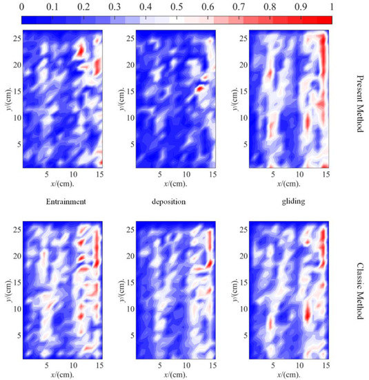
Figure 14.
Spatial distribution of entrained, deposited and gliding particles from left to right in every row, respectively. The figures in top and bottom row are the results calculated by present method and classic method. The flow direction is from bottom to top.
Therefore, the three-step method in this paper makes a deep analysis of the relationship between particle motion and coherent structure possible.
5. Conclusions and Discussion
An improved three-step method has been proposed for identifying and tracking individual active bed-load particles in complex backgrounds. The first two steps, while similar to those used in the classic method, introduces a new algorithm for locating accurate particle centers and Kalman filter for matching particles. The third step serves to find broken chains and to connect them into a complete chain. Locating accurate particle centers reduced the errors caused by high-frequency measurement and facilitates subsequent tracking of particles. The Kalman filter keeps tracking the moving particles, and global connection greatly enhanced the effectiveness of particle tracking.
The present method was validated against simulated images with different parameters. The results of number of active particles, velocities, fight time and length show that the new method successfully solves the new problems caused by frequency and complex background.
The present method has also been used to process real bed-load transport images. Results show that while the classic method tends to underestimate the flight length and time, the new method can provide more accurate information (parameters) on bed-load dynamics than previous methods. As these parameters, e.g., N, L and T, affect not only the transport rate, but also the advection and diffusion characteristics of bed-load transport, the present method shows promise as being a more reliable tool for gaining deeper insight into the physics of bed-load transport.
While the present three-step method proposed can accurately track multiple particles moving above complex background, its performance in practice is affected by factors, such as camera specification, sampling frequency, and size of the observation window. For instance, if the observation window is small, it is impossible to capture the entire flight process of a bed-load particle, and thus the measurements would underestimate the real flight length and durations of moving bed-load particles. Thus, application of the new approach requires more experience and optimization of parameters like the distribution of entrained, gliding and deposited particles.
Author Contributions
Conceptualization, W.M. and Q.Z.; methodology, W.M.; data curation, W.M.; writing—original draft preparation, W.M.; writing—review and editing, W.M.; supervision, D.L.; funding acquisition, D.L. All authors have read and agreed to the published version of the manuscript.
Funding
The research reported herein is funded by National Nature Science Foundation of China (No.51879138 & No.51809268).
Conflicts of Interest
There are no conflict of interest. The funders had no role in the design of the study; in the collection, analyses, or interpretation of data; in the writing of the manuscript, or in the decision to publish the results.
References
- Du Boys, P. Le Rône et les rivires á lit affouiable: Étude du régime du Rhône et de l’action exercée par les eaux sur un lit à fond de graviers indéfiniment affouillable. Ann. Ponts Chaussees 1879, 5, 141–195. [Google Scholar]
- Gilbert, G.K.; Murphy, E.C. The Transportation of Debris by Running Water; US Government Printing Office: Washington, DC, USA, 1914.
- Chien, N.; Wan, Z. Mechanics of Sediment Transport. In Mechanics of Sediment Transport; American Society of Civil Engineers: Reston, VA, USA, 1999. [Google Scholar]
- Drake, T.G.; Shreve, R.L.; Dietrich, W.E.; Leopold, L.B. Bedload transport of fine gravel observed by motion-picture photography. J. Fluid Mech. 1988, 192, 193–217. [Google Scholar] [CrossRef]
- Niño, Y.; García, M.; Ayala, L. Gravel saltation 1. Exp. Water Resour. Res. 1994, 30, 1907–1914. [Google Scholar] [CrossRef]
- Singh, A.; Fienberg, K.; Jerolmack, D.J.; Marr, J.; Foufoula-Georgiou, E. Experimental evidence for statistical scaling and intermittency in sediment transport rates. J. Geophys. Res. 2009, 114, F01025. [Google Scholar] [CrossRef]
- Roseberry, J.C.; Schmeeckle, M.W.; Furbish, D.J. A probabilistic description of the bed load sediment flux: 2. Particle activity and motions. J. Geophys. Res. Earth Surf. 2012. [Google Scholar] [CrossRef]
- Hu, C.H.; Hui, Y.J. Stochastic Feature of Parameters of Particle Saltation. J. Sediment Res. 1990, 4, 1–9. (In Chinese) [Google Scholar]
- Middleton, R.; Brasington, J.; Murphy, B.J.; Frostick, L.E. Monitoring gravel framework dilation using a new digital particle tracking method. Comput. Geosci. 2000. [Google Scholar] [CrossRef]
- Frey, P.; Ducottet, C.; Jay, J. Fluctuations of bed load solid discharge and grain size distribution on steep slopes with image analysis. Exp. Fluids 2003. [Google Scholar] [CrossRef]
- Lajeunesse, E.; Malverti, L.; Charru, F. Bed load transport in turbulent flow at the grain scale: Experiments and modeling. J. Geophys. Res. Earth Surf. 2010. [Google Scholar] [CrossRef]
- Martin, R.L.; Jerolmack, D.J.; Schumer, R. The physical basis for anomalous diffusion in bed load transport. J. Geophys. Res. Earth Surf. 2012. [Google Scholar] [CrossRef]
- Miao, W.; Chen, H.; Chen, Q.G.; Li, D.X. Image-based measurement of bed-load transport in closed channel flow. In Proceedings of the 36th IAHR World Congress, Hague, The Netherlands, 28 June 2015. [Google Scholar]
- Tsubaki, R.; Baranya, S.; Muste, M.; Toda, Y. Spatio-temporal patterns of sediment particle movement on 2D and 3D bedforms. Exp. Fluids 2018. [Google Scholar] [CrossRef]
- Juez, C.; Caviedes-Voullième, D.; Murillo, J.; García-Navarro, P. 2D dry granular free-surface transient flow over complex topography with obstacles. Part II: Numerical predictions of fluid structures and benchmarking. Comput. Geosci. 2014, 73, 142–163. [Google Scholar] [CrossRef]
- Caviedes-Voullième, D.; Juez, C.; Murillo, J.; García-Navarro, P. 2D dry granular free-surface flow over complex topography with obstacles. Part I: Experimental study using a consumer-grade RGB-D sensor. Comput. Geosci. 2014, 73, 177–197. [Google Scholar] [CrossRef]
- Ohmi, K.; Li, H.Y. Particle-tracking velocimetry with new algorithms. Meas. Sci. Technol. 2000, 11, 603–616. [Google Scholar] [CrossRef]
- Campagnol, J.; Radice, A.; Ballio, F. Insight on how bed configuration affects properties of bed load motion. In Proceedings of the ICSE6 Sixth Conference on Scour and Erosion, Paris, France, 27–31 August 2012. [Google Scholar]
- Shim, J.; Duan, J.G. Experimental study of bed-load transport using particle motion tracking. Int. J. Sediment Res. 2017. [Google Scholar] [CrossRef]
- Keshavarzy, A.; Ball, J. An application of image processing in the study of sediment motion. J. Hydraul. Res. 1999. [Google Scholar] [CrossRef]
- Papanicolaou, A.N.; Diplas, P.; Balakrishnan, M.; Dancey, C.L. Computer vision technique for tracking bed load movement. J. Comput. Civ. Eng. 1999. [Google Scholar] [CrossRef]
- Radice, A.; Malavasi, S.; Bailio, F. Solid transport measurements through image processing. Exp. Fluids 2006. [Google Scholar] [CrossRef]
- Heyman, J.; Bohorquez, P.; Ancey, C. Entrainment, motion, and deposition of coarse particles transported by water over a sloping mobile bed. J. Geophys. Res. Earth Surf. 2016, 121, 1931–1952. [Google Scholar] [CrossRef]
- Heyman, J. TracTrac: A fast multi-object tracking algorithm for motion estimation. Comput. Geosci. 2019, 128, 11–18. [Google Scholar] [CrossRef]
- Campagnol, J.; Radice, A.; Nokes, R.; Bulankina, V.; Lescova, A.; Ballio, F. Lagrangian analysis of bed-load sediment motion: Database contribution. J. Hydraul. Res. 2013. [Google Scholar] [CrossRef]
- Böhm, T.; Frey, P.; Ducottet, C.; Ancey, C.; Jodeau, M.; Reboud, J.L. Two-dimensional motion of a set of particles in a free surface flow with image processing. Exp. Fluids 2006. [Google Scholar] [CrossRef]
- Zimmermann, A.E.; Church, M.; Hassan, M.A. Video-based gravel transport measurements with a flume mounted light table. Earth Surf. Process. Landf. 2008. [Google Scholar] [CrossRef]
- Nikora, V.; Habersack, H.; Huber, T.; McEwan, I. On bed particle diffusion in gravel bed flows under weak bed load transport. Water Resour. Res. 2002, 38, 1–17. [Google Scholar] [CrossRef]
- Jonker, R.; Volgenant, A. A shortest augmenting path algorithm for dense and sparse linear assignment problems. Computing 1987, 38, 325–340. [Google Scholar] [CrossRef]
- Prashanth, H.S.; Shashidhara, H.L.; Balasubramanya Murthy, K.N. Prashanth H S, Shashidhara H L, KN B M. Image scaling comparison using universal image quality index. In Proceedings of the 2009 International Conference on Advances in Computing, Control, and Telecommunication Technologies, Trivandrum, India, 28–29 December 2009; pp. 859–863. [Google Scholar]
- Welch, G.; Bishop, G. (Department of Computer Science, University of North Carolina, Chapel Hill, NC, USA). An introduction to the Kalman filter. Personal communication, 1995. [Google Scholar] [CrossRef]
- Miao, W.; Cao, L.; Zhong, Q.; Li, D. Influence of the time interval on image-based measurement of bed-load transport. J. Hydraul. Res. 2018. [Google Scholar] [CrossRef]
- Ancey, C. Stochastic modeling in sediment dynamics: Exner equation for planar bed incipient bed load transport conditions. J. Geophys. Res. Earth Surf. 2010. [Google Scholar] [CrossRef]
- Tregnaghi, M.; Bottacin-Busolin, A.; Tait, S.; Marion, A. Stochastic determination of entrainment risk in uniformly sized sediment beds at low transport stages: 2. Experiments. J. Geophys. Res. 2012, 117, 1–17. [Google Scholar] [CrossRef]
- Sun, H.G.; Chen, D.; Zhang, Y.; Chen, L. Understanding partial bed-load transport: Experiments and stochastic model analysis. J. Hydrol. 2015. [Google Scholar] [CrossRef]
- Miao, W.; Cao, L.K.; Chen, Q.G.; Li, D.X. Parameter optimization for image-based measurement of bed-load transport in pressurized closed channel flow. J. Exp. Fluid Mech. 2017, 31, 80–86. (In Chinese) [Google Scholar]
- Zhong, Q.; Chen, Q.; Wang, H.; Li, D.; Wang, X. Statistical analysis of turbulent super-streamwise vortices based on observations of streaky structures near the free surface in the smooth open channel flow. Water Resour. Res. 2016, 52, 3563–3578. [Google Scholar] [CrossRef]
© 2020 by the authors. Licensee MDPI, Basel, Switzerland. This article is an open access article distributed under the terms and conditions of the Creative Commons Attribution (CC BY) license (http://creativecommons.org/licenses/by/4.0/).