Optimization Design of the Mix Ratio of a Nano-TiO2/CaCO3-Basalt Fiber Composite Modified Asphalt Mixture Based on Response Surface Methodology

Abstract
1. Introduction
2. Materials and Methods
2.1. Raw Materials
2.1.1. Asphalt
2.1.2. Basalt Fiber
2.1.3. Nanomaterials
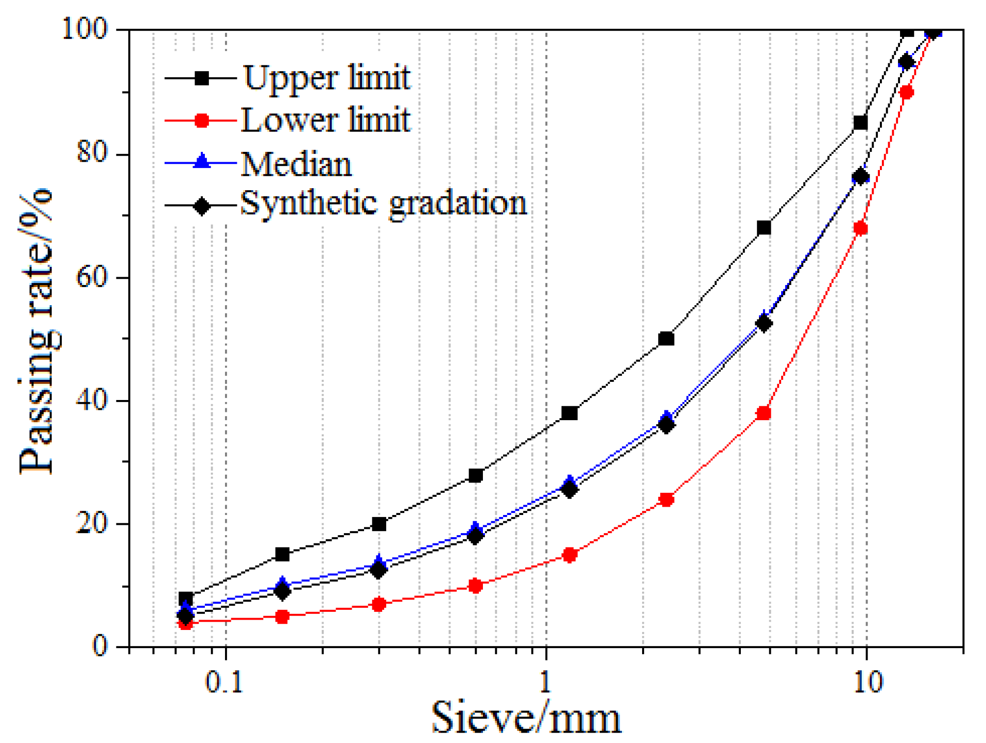
2.1.4. Aggregates and Fillers
2.2. Response Surface Methodology
2.3. Test Design
2.4. Response Output Index Test Method
2.4.1. Production of Asphalt Mixture Test Piece
2.4.2. Measurement and Calculation of the Volume Index
2.4.3. Determination of Marshall Stability Test Index
3. Results and Discussion
3.1. Analysis of Response Output Index Results
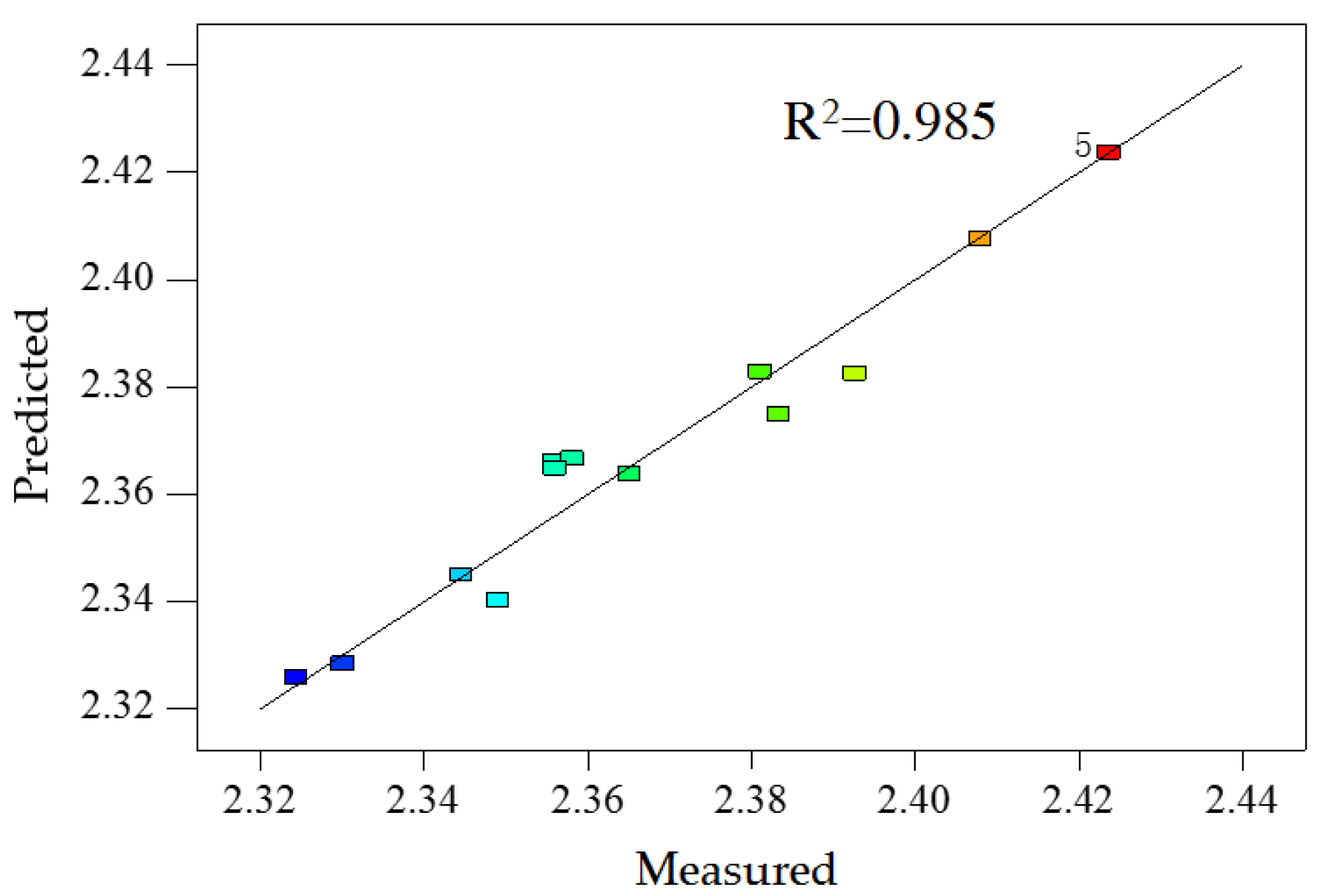
3.1.1. Density
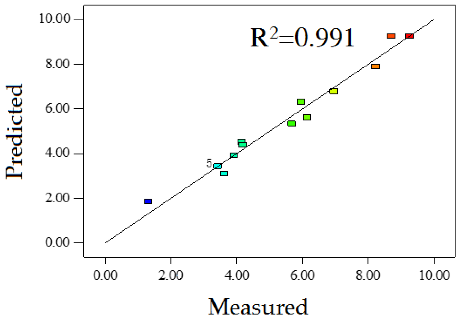
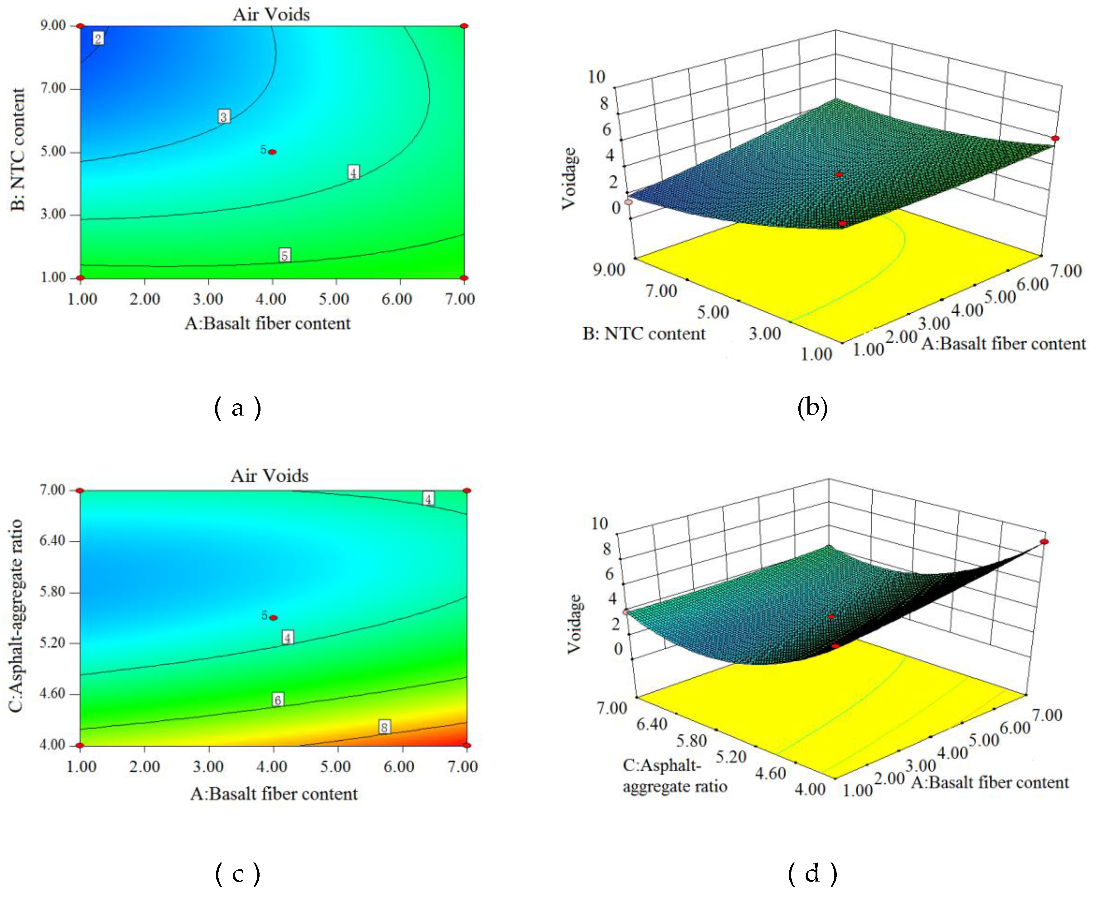
3.1.2. Air Voids
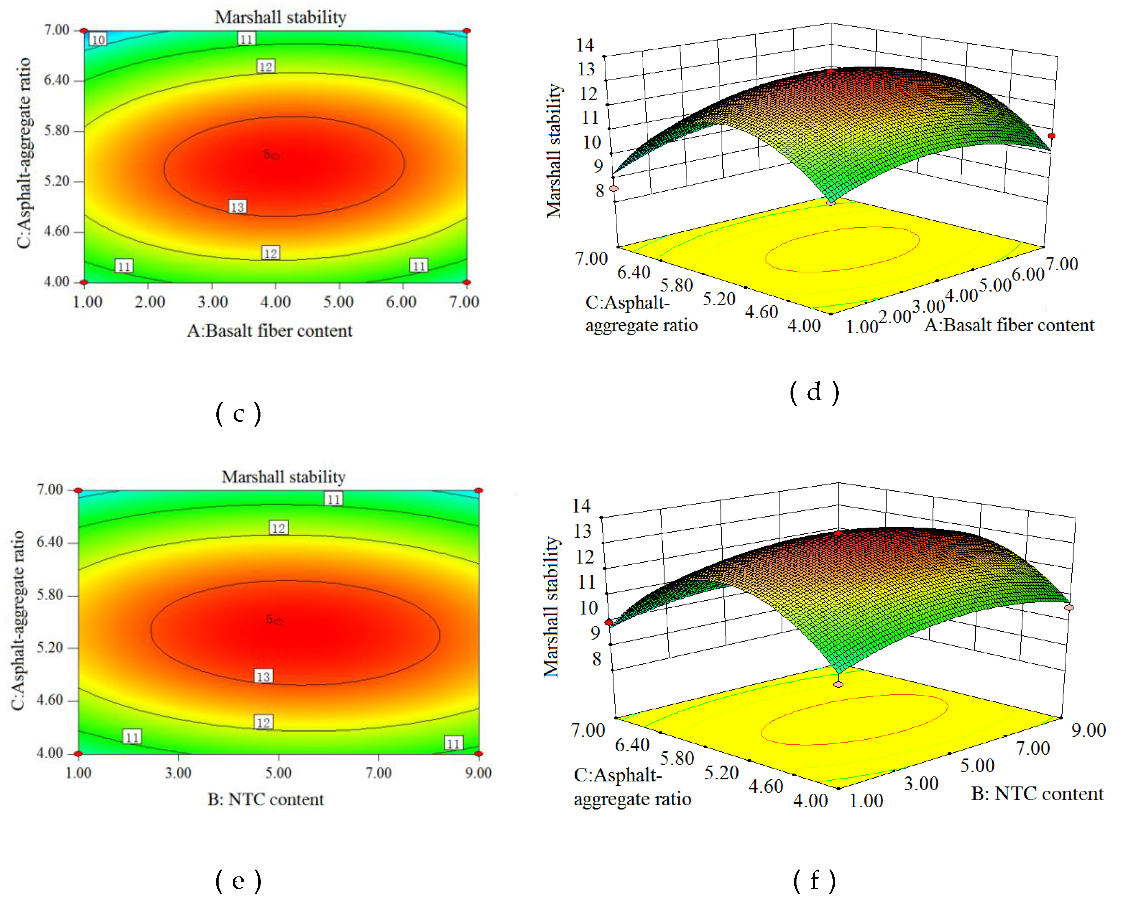
3.1.3. Marshall Stability
3.1.4. Three Other Response Indicators
3.2. Input Index Optimization Based on Response Surface Fitting Model
3.3. Model Validation
4. Conclusions
Author Contributions
Funding
Acknowledgments
Conflicts of Interest
References
- Huang, B.; Ma, L.P.; Xu, W.J. Research Development of Modified Asphalt. Mater. Her. 2010, 24, 137–141. [Google Scholar]
- Chang, H.Z.; Zhang, H.L. Research on Performance and Mechanism of Nano−CaCO3/SBS Composite Modified Asphalt. Highw. Transp. Technol. Appl. Technol. Ed. 2013, 9, 28–31. [Google Scholar]
- Manias, E.; Touny, A.; Wu, L.; Lu, B.; Strawhecker, K.; Gilman, J.W.; Chung, T.C. Polypropylene/Silicate Nanocomposites, Synthetic Routes and Materials Properties. Chem. Mater. 2001, 13, 3516–3523. [Google Scholar] [CrossRef]
- Raufi, H.; Topal, A.; Kaya, D.; Sengoz, B. Performance Evaluation of Nano−CaCO3 Modified Bitumen in Hot Mix Asphalt. In Proceedings of the 18th IRF World Road Meeting, Delhi, India, 14–17 November 2017. [Google Scholar]
- Nejad, F.M.; Nazari, H.; Naderi, K.; Karimiyan Khosroshahi, F.; Hatefi Oskuei, M. Thermal and rheological properties of nanoparticle modified asphalt binder at low and intermediate temperature range. Pet. Sci. Technol. 2017, 35, 641–646. [Google Scholar] [CrossRef]
- Shafabakhsh, G.; Mirabdolazimi, S.M.; Sadeghnejad, M. Evaluation the effect of nano−TiO2 on the rutting and fatigue behavior of asphalt mixtures. Constr. Build. Mater. 2014, 54, 566–571. [Google Scholar] [CrossRef]
- Azarhoosh, A.R.; Nejad, F.M.; Khodaii, A. Using the Surface Free Energy Method to Evaluate the Effects of Nanomaterial on the Fatigue Life of Hot Mix Asphalt. J. Mater. Civ. Eng. 2016, 28, 04016098.1–04016098.9. [Google Scholar] [CrossRef]
- Sun, L.; Xin, X.T.; Wang, H.Y.; Gu, W.J. Performance of nanomaterials modified asphalt binders. J. Chin. Ceram. Soc. 2012, 40, 1095–1101. [Google Scholar]
- Sun, L.; Xin, X.T.; Ren, J.L. Road performance of nano−modified asphalt mixture. J. Southeast Univ. Nat. Sci. Ed. 2013, 4, 203–206. [Google Scholar]
- Ye, C.; Chen, H.X.; Wang, C. Research on Road Performance of Nano−TiO2 Modified Asphalt Mixture. Sino Foreign Highw. 2010, 3, 322–325. [Google Scholar]
- Ye, C.; Chen, H.X. Research on Road Performance of Nano−SiO2 and Nano−TiO2 Modified Asphalt. New Build. Mater. 2009, 36, 82–84. [Google Scholar]
- Yang, H.H.; Yuan, H.W.; Hao, P.W. Research on road performance of lignin fiber asphalt mixture. Highw. Transp. Sci. Technol. 2003, 20, 10–11. [Google Scholar]
- Wu, J.R.; Qi, D.J. Effect of polyester fiber content and freeze−thaw cycle on the water stability of asphalt mixtures. Silic. Bull. 2017, 4, 311–315. [Google Scholar]
- Zhao, Y.H.; Zhao, L.D.; Fan, Y.F.; Guo, N.S. High temperature and water stability of polyester fiber modified asphalt mixture. J. Build. Mater. 2008, 5, 51–55. [Google Scholar]
- Liu, S. Research on Road Performance of Glass Fiber Asphalt Mixture. Master’s Thesis, Chongqing Jiaotong University, Chongqing, China, 2016. [Google Scholar]
- Li, L.Q. Application of basalt fiber in asphalt pavement of long uphill section. J. Zhejiang Jiaotong Vocat. Tech. Coll. 2011, 3, 20–22. [Google Scholar]
- Wu, S.P.; Ye, Q.S.; Liu, Z.F. Research on mineral fiber to improve the high temperature stability of asphalt mixture. Highw. Transp. Sci. Technol. 2008, 11, 24–27. [Google Scholar]
- Cheng, Y.; Zhu, C.; Tan, G.; Lv, Z.; Yang, J.; Ma, J. Laboratory Study on Properties of Diatomite and Basalt Fiber Compound Modified Asphalt Mastic. Adv. Mater. Sci. Eng. 2017, 2017, 1–10. [Google Scholar] [CrossRef]
- Qin, X.; Shen, A.; Guo, Y.; Li, Z.; Lv, Z. Characterization of asphalt mastics reinforced with basalt fibers. Constr. Build. Mater. 2018, 159, 508–516. [Google Scholar] [CrossRef]
- Wu, Z.G.; Xia, Y.; Lu, R.Y.; Lu, Y.F.; Cao, J.W. Experimental study on the performance of graded basalt fiber reinforced modified asphalt mixture. Constr. Technol. 2018, 47, 62–65 + 76. [Google Scholar]
- Ren, G.M.; Gu, X.Y.; Tian, P. Research on fatigue performance of basalt fiber asphalt mortar. Highw. Transp. Sci. Technol. Appl. Technol. Ed. 2012, 4, 78–79. [Google Scholar]
- Yang, J.S. Research on Road Performance and Low Temperature Characteristics of Basalt Fiber SMA−13. Master’s Thesis, Jilin University, Changchun, China, 2018. [Google Scholar]
- Wang, D.; Linbing, W.; Christian, D.; Zhou, G. Fatigue Properties of Asphalt Materials at Low In−Service Temperatures. J. Mater. Civ. Eng. 2013, 25, 1220–1227. [Google Scholar] [CrossRef]
- Gu, X.; Xu, T.; Ni, F. Rheological Behavior of Basalt Fiber Reinforced Asphalt Mastic. J. Wuhan Univ. Technol. Mater. Sci. Ed. 2014, 29, 950–955. [Google Scholar] [CrossRef]
- Gao, C.M. Research on the Performance of Basalt Fiber Asphalt Concrete and Microscopic Analysis of the Strengthening Mechanism. Master’s Thesis, Jilin University, Changchun, China, 2012. [Google Scholar]
- Zhang, X.Y.; Gu, X.Y.; Lv, J.X. Effect of basalt fiber distribution on the flexural−tensile Theological performance of asphalt mortar. Constr. Build. Mater. 2018, 179, 307–314. [Google Scholar] [CrossRef]
- Zhang, X.; Gu, X.; Lv, J.; Zou, X. 3D numerical model to investigate the rheological properties of basalt fiber reinforced asphalt−like materials. Constr. Build. Mater. 2017, 138, 185–194. [Google Scholar] [CrossRef]
- Omranian, S.R.; Hamzah, M.O.; Valentin, J.; Hasan, M.R.M. Determination of optimal mix from the standpoint of short term aging based on asphalt mixture fracture properties using response surface method. Constr. Build. Mater. 2018, 179, 35–48. [Google Scholar] [CrossRef]
- Kim, D.H.; Jeong, E.; Oh, S.E.; Shin, H.S. Combined (alkaline + ultrasonic) pretreatment effect on sewage sludge disintegration. Water Res. 2010, 44, 3093–3100. [Google Scholar] [CrossRef]
- Kushwaha, J.P.; Srivastava, V.C.; Mall, I.D. Organics removal from dairy waste water by electrochemical treatment and residue disposal. Sep. Purif. Technol. 2010, 76, 198–205. [Google Scholar] [CrossRef]
- Wang, W.; Cheng, Y.; Tan, G. Design Optimization of SBS−Modified Asphalt Mixture Reinforced with Eco−Friendly Basalt Fiber Based on Response Surface Methodology. Materials 2018, 11, 1311. [Google Scholar] [CrossRef]
- Valencia, L.E.C.; Ramirez, A.M.; Guzman, E.A.; Garcia, M.E.C. Modelling of the performance of asphalt pavement using response surface methodology−the kinetics of the aging. Build. Environ. 2007, 42, 933–999. [Google Scholar] [CrossRef]
- Moghaddam, T.B.; Soltani, M.; Karim, M.R.; Baaj, H. Optimization of asphalt and modifier contents for polyethylene terephthalate modified asphalt mixtures using response surface methodology. Measurement 2015, 74, 159–169. [Google Scholar] [CrossRef]
- JTG E20−2011. Standard Test Methods of Asphalt and Asphalt Mixtures for Highway Engineering; Ministry of Transport: Beijing, China, 2011. (In Chinese)
- GB/T 38111−2019. Classification, Gradation and Designation of Basalt Fiber; National Standardization Management Committee: Beijing, China, 2019. (In Chinese)
- JTG E42−2005. Test Methods of Aggregate for Highway Engineering; Ministry of Transport: Beijing, China, 2005. (In Chinese)
- Zhang, Z.Z.; Han, C.L.; Li, C.W. Application of Response Surface Method in Experimental Design, and Optimization Application of Response Surface Method in Experimental Design and Optimization. J. Henan Educ. Inst. Nat. Sci. Ed. 2011, 20, 34–37. [Google Scholar]
- Gong, Y.; Bi, H.; Tian, Z.; Tan, G. Pavement Performance Investigation of Nano−TiO2/CaCO3 and Basalt Fiber Composite Modified Asphalt Mixture under Freeze‒Thaw Cycles. Appl. Sci. 2018, 8, 2581. [Google Scholar] [CrossRef]
- Liu, D.L.; Yue, A.J.; Chen, L. Study on the properties of nano−calcium carbonate modified asphalt and its mixture. J. Chang. Jiaotong Univ. 2004, 18, 70–72. [Google Scholar]
- Ni, P. Design and Road Performance Test of Basalt Fiber SMA−13 Mixture. Master’s Thesis, Jilin University, Changchun, China, 2017. [Google Scholar]
- Sun, X. Research on the properties of diatomaceous earth/basalt fiber composite modified asphalt and asphalt mixture. New Build. Mater. 2019, 46, 90–94. [Google Scholar]
- JTG F40−2004. Technical Specifications for Construction of Highway Asphalt Pavements; Ministry of Transport: Beijing, China, 2004. (In Chinese)


| Index | Result | Specification Limit |
|---|---|---|
| Penetration (25 °C, 5 s, 0.1 mm) | 85.8 | 80–100 |
| Softening Point TR&B (°C) | 46.9 | ≥45 |
| Ductility (25 °C, cm) | >150 | ≥100 |
| Brinell Viscosity (135 °C, Pa·s) | 306.9 | —— |
| Density (15 °C, g/cm3) | 1.016 | —— |
| Index | Result | Specification Limit |
|---|---|---|
| Diameter (μm) | 10–13 | —— |
| Length (mm) | 6 | —— |
| Water Content (%) | 0.030 | ≤0.2 |
| Combustible Content (%) | 0.56 | —— |
| Linear Density (Tex) | 2398 | 2400 ± 120 |
| Breaking Strength (N/Tex) | 0.55 | ≥0.40 |
| Tensile Strength (MPa) | 2320 | ≥2000 |
| Tensile Elastic Modulus (GPa) | 86.3 | ≥85 |
| Breaking Elongation (%) | 2.84 | ≥2.5 |
| Sieve Size/mm | 13.2 | 9.5 | 4.75 | 2.36 | 1.18 | 0.6 | 0.3 | 0.15 | 0.075 |
|---|---|---|---|---|---|---|---|---|---|
| Apparent Relative Density γa | 3.142 | 2.992 | 3.084 | 2.721 | 2.661 | 2.758 | 2.684 | 2.907 | 2.627 |
| Relative Density of Surface Stem γs | 3.066 | 2.943 | 3.001 | 2.646 | 2.602 | 2.709 | 2.635 | 2.820 | 2.528 |
| Relative Density of Gross Volume γb | 3.031 | 2.917 | 2.961 | 2.603 | 2.566 | 2.681 | 2.606 | 2.776 | 2.476 |
| Water Absorption wx (%) | 1.17 | 0.86 | 1.35 | 1.67 | 1.38 | 1.07 | 1.13 | 2.14 | 2.04 |
| Index | Unit | Measured Value | Specification Requirements (Highway Surface Layer) |
|---|---|---|---|
| Apparent Relative Density | g/cm3 | 2.719 | ≥2.5 |
| Water Content | % | 0.19 | ≤1 |
| Size Range < 0.6 mm | % | 100 | 100 |
| <0.15 | % | 95.1 | 90–100 |
| <0.075 | % | 87.8 | 75–100 |
| Outward Appearance | No agglomeration | No agglomeration | |
| Hydrophilic Coefficient | 0.68 | <1 |
| Technical Index | Measured Value | Specification Limit |
|---|---|---|
| Crush Value (%) | 13.5 | ≤28 |
| Wear Value (%) | 16.0 | ≤30 |
| Impact Factor | Name | Unit | Minimum | Maximum | Level |
|---|---|---|---|---|---|
| −1 0 1 | |||||
| A | Fiber Content | % | 1.00 | 7.00 | 1.0 4.0 7.0 |
| B | NTC Content | % | 1.00 | 9.00 | 1.0 5.0 9.0 |
| C | Asphalt–aggregate ratio | % | 4.00 | 7.00 | 4.0 5.5 7.0 |
| Numbering | BF Content (%) | NTC Content (%) | Asphalt–Aggregate Ratio (%) |
|---|---|---|---|
| 1 | 1.0 | 5.0 | 4.0 |
| 2 | 1.0 | 5.0 | 7.0 |
| 3 | 4.0 | 5.0 | 5.5 |
| 4 | 7.0 | 5.0 | 7.0 |
| 5 | 4.0 | 5.0 | 5.5 |
| 6 | 4.0 | 1.0 | 7.0 |
| 7 | 1.0 | 9.0 | 5.5 |
| 8 | 4.0 | 9.0 | 4.0 |
| 9 | 4.0 | 1.0 | 4.0 |
| 10 | 7.0 | 5.0 | 4.0 |
| 11 | 1.0 | 1.0 | 5.5 |
| 12 | 7.0 | 1.0 | 5.5 |
| 13 | 4.0 | 5.0 | 5.5 |
| 14 | 4.0 | 5.0 | 5.5 |
| 15 | 4.0 | 5.0 | 5.5 |
| 16 | 7.0 | 9.0 | 5.5 |
| 17 | 4.0 | 9.0 | 7.0 |
| Test Serial Number | A | B | C | Density (g/cm3) | Air Voids (%) | Marshall Stability (kN) | Flow Value (mm) | VMA (%) | VFA (%) |
|---|---|---|---|---|---|---|---|---|---|
| 1 | 1.0 | 5.0 | 4.0 | 2.383 | 6.9 | 10.30 | 1.9 | 13.0 | 46.5 |
| 2 | 1.0 | 5.0 | 7.0 | 2.365 | 3.9 | 8.57 | 3.6 | 16.1 | 75.6 |
| 3 | 4.0 | 5.0 | 5.5 | 2.423 | 3.4 | 13.37 | 2.5 | 12.8 | 73.2 |
| 4 | 7.0 | 5.0 | 7.0 | 2.358 | 4.2 | 9.73 | 2.7 | 16.3 | 74.3 |
| 5 | 4.0 | 5.0 | 5.5 | 2.423 | 3.4 | 13.37 | 2.5 | 12.8 | 73.2 |
| 6 | 4.0 | 1.0 | 7.0 | 2.349 | 5.9 | 9.92 | 3.7 | 16.6 | 64.2 |
| 7 | 1.0 | 9.0 | 5.5 | 2.408 | 1.3 | 12.10 | 2.9 | 12.2 | 89.2 |
| 8 | 4.0 | 9.0 | 4.0 | 2.356 | 8.2 | 10.53 | 1.8 | 14.0 | 41.2 |
| 9 | 4.0 | 1.0 | 4.0 | 2.330 | 8.7 | 9.83 | 2.3 | 14.9 | 41.8 |
| 10 | 7.0 | 5.0 | 4.0 | 2.324 | 9.2 | 10.79 | 2.1 | 15.1 | 38.9 |
| 11 | 1.0 | 1.0 | 5.5 | 2.355 | 5.6 | 11.52 | 2.8 | 15.2 | 62.7 |
| 12 | 7.0 | 1.0 | 5.5 | 2.344 | 6.1 | 11.65 | 2.6 | 15.6 | 60.7 |
| 13 | 4.0 | 5.0 | 5.5 | 2.423 | 3.4 | 13.37 | 2.5 | 12.8 | 73.2 |
| 14 | 4.0 | 5.0 | 5.5 | 2.430 | 3.4 | 13.37 | 2.5 | 12.8 | 73.2 |
| 15 | 4.0 | 5.0 | 5.5 | 2.430 | 3.4 | 13.37 | 2.5 | 12.8 | 73.2 |
| 16 | 7.0 | 9.0 | 5.5 | 2.392 | 4.1 | 11.15 | 3.3 | 13.2 | 68.4 |
| 17 | 4.0 | 9.0 | 7.0 | 2.381 | 3.6 | 10.06 | 2.4 | 15.5 | 76.6 |
| Project | Name | Unit | Min. | Max. | Average | Standard Deviation |
|---|---|---|---|---|---|---|
| Y1 | Density | g/cm3 | 2.324 | 2.431 | 2.380 | 0.0355 |
| Y2 | Air Voids | % | 1.3 | 9.3 | 5.0 | 2.2226 |
| Y3 | Marshall Stability | kN | 8.57 | 13.38 | 11.36 | 1.5741 |
| Y4 | Flow Value | mm | 1.8 | 3.7 | 2.7 | 0.5265 |
| Y5 | VMA | % | 12.3 | 16.7 | 14.3 | 1.5146 |
| Y6 | VFA | % | 38.9 | 89.2 | 65.1 | 14.6017 |
| Types | Continuous P Value | Out-of-Fit P Value | Correct R2 | Predict R2 | Result |
|---|---|---|---|---|---|
| Linear | 0.3169 | <0.0001 | 0.0528 | −0.1622 | — |
| 2FI | 0.9247 | <0.0001 | −0.1768 | −0.9142 | — |
| Quadratic | <0.0001 | <0.0001 | 0.9416 | 0.5912 | Recommended |
| Source of Variance | Sum of Squares | Degrees of Freedom | Mean Square | F Value | Probability > F | Result |
|---|---|---|---|---|---|---|
| Mean vs. Total | 96.3291 | 1 | 96.3291 | — | — | — |
| Linear vs. Mean | 0.0046 | 3 | 0.0015 | 1.2978 | 0.3169 | — |
| 2FI vs. Linear | 0.0006 | 3 | 0.0002 | 0.1540 | 0.9247 | — |
| Quadratic vs. 2FI | 0.0143 | 3 | 0.0047 | 64.8540 | <0.0001 | Recommended |
| Residual | 2.59 × 10⁻¹² | 4 | 6.48 × 10⁻¹³ | — | — | — |
| Total | 96.349 | 17 | 5.6676 | — | — | — |
| Source of Variance | Sum of Squares | Degrees of Freedom | Mean Square | F Value | Probability > F | Result |
|---|---|---|---|---|---|---|
| Linear | 0.0155 | 9 | 0.0017 | 2.65 × 10⁻⁹ | <0.0001 | — |
| 2FI | 0.0148 | 6 | 0.0024 | 3.81 × 10⁻⁹ | <0.0001 | — |
| Quadratic | 0.0005 | 3 | 0.0001 | 2.64 × 10⁻⁸ | <0.0001 | Recommended |
| Pure error | 2.59 × 10⁻¹² | 4 | 6.48 × 10⁻¹³ | — | — | — |
| Types | Sample Standard Deviation | Fit | Corrected Fit | Prediction Fit | Result |
|---|---|---|---|---|---|
| Linear | 0.0345 | 0.2304 | 0.0528 | -0.1622 | — |
| 2FI | 0.0385 | 0.2644 | −0.1768 | −0.9142 | — |
| Quadratic | 0.0085 | 0.9744 | 0.9416 | 0.5912 | Recommended |
| Cubic | 8.0538 × 10⁻⁷ | 1 | 0.9999 | — | Poor |
| Project | Sum of Squares | Degrees of Freedom | Mean Square Error | F Value | P Value | Significant |
|---|---|---|---|---|---|---|
| Model | 0.02 | 9 | 2.18 × 10⁻³ | 29.67 | <0.0001 | √ |
| A: Fiber Content | 1.08 × 10⁻³ | 1 | 1.08 × 10⁻³ | 14.6 | 0.0065 | √ |
| B: Nano-Material Content | 3.13 × 10⁻³ | 1 | 3.13 × 10⁻³ | 42.5 | 0.0003 | √ |
| C: Asphalt–Aggregate Ratio | 4.46 × 10⁻⁴ | 1 | 4.46 × 10⁻⁴ | 6.06 | 0.0434 | √ |
| AB | 3.96 × 10⁻⁶ | 1 | 3.96 × 10⁻⁶ | 0.054 | 0.8233 | × |
| AC | 6.72 × 10⁻⁴ | 1 | 6.72 × 10⁻⁴ | 9.14 | 0.0193 | √ |
| BC | 9.27 × 10⁻⁶ | 1 | 9.27 × 10⁻⁶ | 0.13 | 0.7331 | × |
| A^2 | 2.11 × 10⁻³ | 1 | 2.11 × 10⁻³ | 28.64 | 0.0011 | √ |
| B^2 | 2.86 × 10⁻³ | 1 | 2.86 × 10⁻³ | 38.88 | 0.0004 | √ |
| C^2 | 8.01 × 10⁻³ | 1 | 8.01 × 10⁻³ | 108.77 | <0.0001 | √ |
| Residual | 5.15 × 10⁻⁴ | 7 | 7.36 × 10⁻⁵ | — | — | — |
| Mismatch | 5.15 × 10⁻⁴ | 3 | 1.72 × 10⁻⁴ | — | — | — |
| Pure Error | 0 | 4 | 0 | — | — | — |
| Total Deviation | 0.02 | 16 | — | — | — | — |
| Project | Sum of Squares | Degrees of Freedom | Mean Square Error | F Value | P Value | Significant |
|---|---|---|---|---|---|---|
| Model | 77.35 | 9 | 8.59 | 35.59 | <0.0001 | √ |
| A: Fiber Content | 4.32 | 1 | 4.32 | 17.9 | 0.0039 | √ |
| B: Nano-Material Content | 10.46 | 1 | 10.46 | 43.31 | 0.0003 | √ |
| C: Asphalt–Aggregate Ratio | 29.83 | 1 | 29.83 | 123.52 | <0.0001 | √ |
| AB | 1.42 | 1 | 1.42 | 5.87 | 0.0459 | √ |
| AC | 1.01 | 1 | 1.01 | 4.2 | 0.0797 | × |
| BC | 0.86 | 1 | 0.86 | 3.56 | 0.1013 | × |
| A^2 | 0.13 | 1 | 0.13 | 0.53 | 0.4909 | × |
| B^2 | 2.2 | 1 | 2.2 | 9.11 | 0.0194 | √ |
| C^2 | 25.86 | 1 | 25.86 | 107.08 | <0.0001 | √ |
| Residual | 1.69 | 7 | 0.24 | — | — | — |
| Mismatch | 1.69 | 3 | 0.56 | — | — | — |
| Pure Error | 0 | 4 | 0 | — | — | — |
| Total Deviation | 79.04 | 16 | — | — | — | — |
| Project | Sum of Squares | Degrees of Freedom | Mean Square Error | F Value | P Value | Significant |
|---|---|---|---|---|---|---|
| Model | 38.08 | 9 | 4.23 | 18.95 | 0.0004 | √ |
| A: Fiber Content | 0.086 | 1 | 0.086 | 0.39 | 0.5543 | × |
| B: Nano-Material Content | 0.11 | 1 | 0.11 | 0.48 | 0.5112 | × |
| C: Asphalt–aggregate Ratio | 1.25 | 1 | 1.25 | 5.61 | 0.0497 | √ |
| AB | 0.29 | 1 | 0.29 | 1.29 | 0.2928 | × |
| AC | 0.11 | 1 | 0.11 | 0.51 | 0.4982 | × |
| BC | 0.076 | 1 | 0.076 | 0.34 | 0.5788 | × |
| A^2 | 4.24 | 1 | 4.24 | 19 | 0.0033 | √ |
| B^2 | 2.46 | 1 | 2.46 | 11.04 | 0.0127 | √ |
| C^2 | 26.79 | 1 | 26.79 | 119.98 | <0.0001 | √ |
| Residual | 1.56 | 7 | 0.22 | — | — | — |
| Mismatch | 1.56 | 3 | 0.52 | — | — | — |
| Pure Error | 0 | 4 | 0 | — | — | — |
| Total Deviation | 39.64 | 16 | — | — | — | — |
| Fiber Content (%) | NTC Content (%) | Asphalt–Aggregate Ratio (%) | Density (g/cm3) | Air Voids (%) | Marshall Stability (kN) | Flow Value (mm) | VMA (%) | VFA (%) |
|---|---|---|---|---|---|---|---|---|
| 3.9 | 5.1 | 5.67 | 2.4237 | 3.4 | 13.29 | 2.7 | 14.9 | 73.2 |
| Project | Density (g/cm3) | Air Voids (%) | Marshall Stability (kN) | Flow Value (mm) | VMA (%) | VFA (%) |
|---|---|---|---|---|---|---|
| 1 | 2.431 | 3.436 | 17.22 | 1.8 | 16.7 | 56.9 |
| 2 | 2.399 | 4.516 | 12.59 | 2.3 | 14.6 | 84.2 |
| 3 | 2.497 | 4.593 | 16.13 | 2.9 | 13.9 | 80.1 |
| 4 | 2.428 | 5.22 | 15.62 | 1.9 | 12.3 | 71.6 |
| 5 | 2.429 | 1.384 | 11.75 | 3.8 | 15.6 | 77.3 |
| 6 | 2.396 | 1.413 | 11.71 | 4.7 | 13.9 | 67.3 |
| Average Value | 2.430 | 3.427 | 14.17 | 2.9 | 14.5 | 72.9 |
| Standard Deviation | 0.033 | 1.527 | 2.223 | 1.050 | 1.392 | 9.018 |
| Prediction Data | 2.424 | 3.43 | 13.29 | 2.7 | 14.9 | 73.2 |
| Error (%) | 0.270 | 0.096 | 6.620 | 6.960 | 2.759 | 0.370 |
© 2020 by the authors. Licensee MDPI, Basel, Switzerland. This article is an open access article distributed under the terms and conditions of the Creative Commons Attribution (CC BY) license (http://creativecommons.org/licenses/by/4.0/).
Share and Cite
Gong, Y.; Song, J.; Bi, H.; Tian, Z. Optimization Design of the Mix Ratio of a Nano-TiO2/CaCO3-Basalt Fiber Composite Modified Asphalt Mixture Based on Response Surface Methodology. Appl. Sci. 2020, 10, 4596. https://doi.org/10.3390/app10134596
Gong Y, Song J, Bi H, Tian Z. Optimization Design of the Mix Ratio of a Nano-TiO2/CaCO3-Basalt Fiber Composite Modified Asphalt Mixture Based on Response Surface Methodology. Applied Sciences. 2020; 10(13):4596. https://doi.org/10.3390/app10134596
Chicago/Turabian StyleGong, Yafeng, Jiaxiang Song, Haipeng Bi, and Zhenhong Tian. 2020. "Optimization Design of the Mix Ratio of a Nano-TiO2/CaCO3-Basalt Fiber Composite Modified Asphalt Mixture Based on Response Surface Methodology" Applied Sciences 10, no. 13: 4596. https://doi.org/10.3390/app10134596
APA StyleGong, Y., Song, J., Bi, H., & Tian, Z. (2020). Optimization Design of the Mix Ratio of a Nano-TiO2/CaCO3-Basalt Fiber Composite Modified Asphalt Mixture Based on Response Surface Methodology. Applied Sciences, 10(13), 4596. https://doi.org/10.3390/app10134596