CFD Analysis of Subcooled Flow Boiling in 4 × 4 Rod Bundle


Abstract
1. Introduction
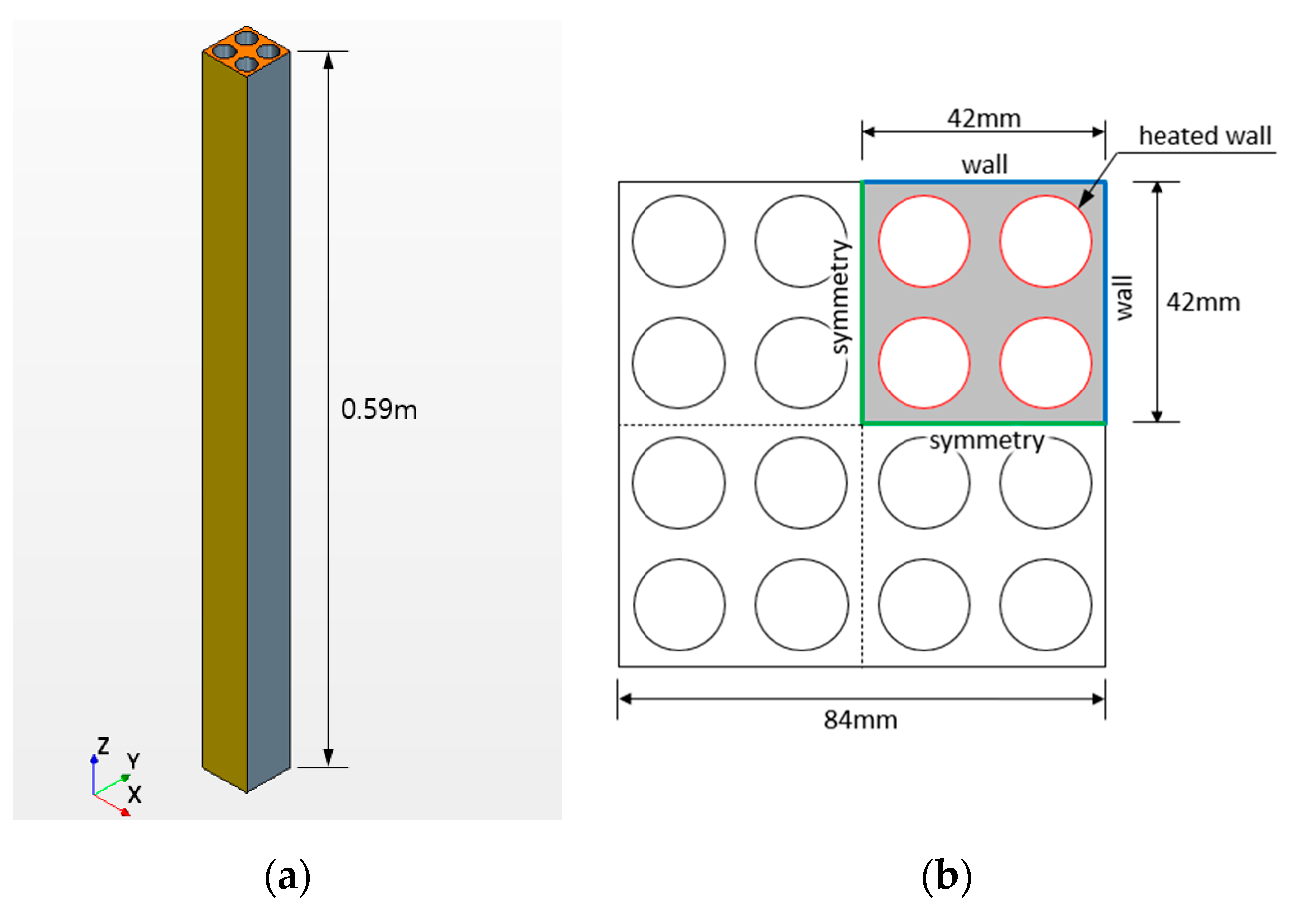
2. Subcooled Boiling Experiment in 4 × 4 Rod Bundle
3. Numerical Methods
3.1. Turbulence Model
3.2. Two-Phase Interaction Models
3.3. Bubble Diameter Model
4. Operating Conditions
4.1. Initial and Boundary Conditions
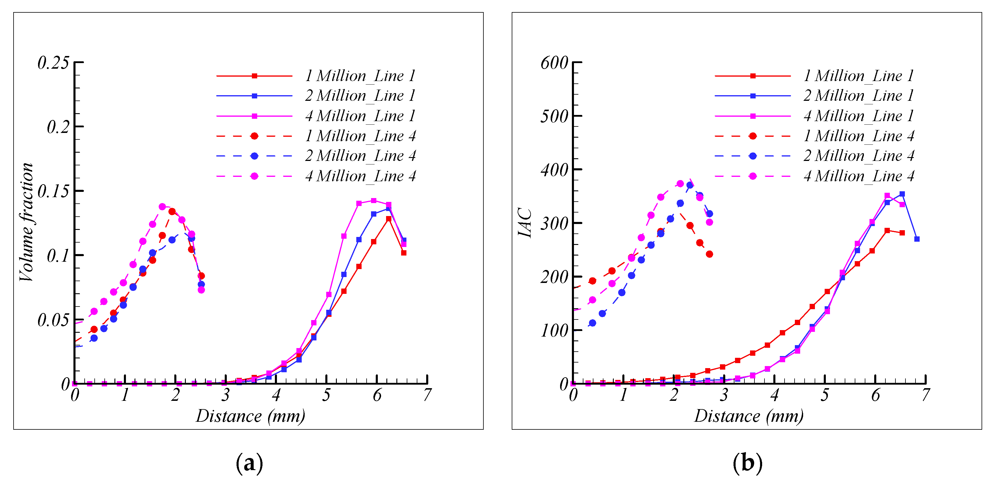
4.2. Grid Test
5. Results
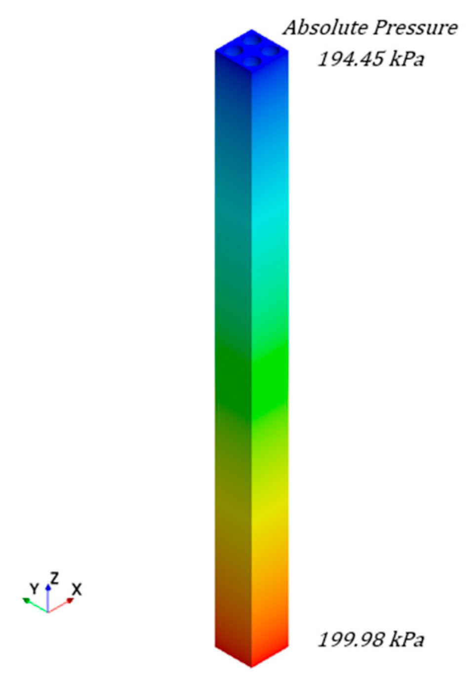
5.1. Results
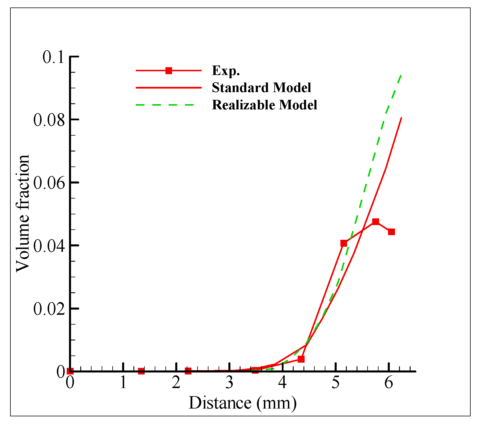
5.2. Model Validation
6. Conclusions
- It enables various water–air flow analyses of low- and high-pressure conditions of the model used in numerical analysis.
- When the error rate is very small in a wide flow path, and the inlet temperature is high or the heat flux is large, the flow boiling phenomenon is properly predicted.
- Through an analysis of vertical plane flow, which cannot be measured by experiments, the cause of the high-volume fraction at the edge was investigated by using the liquid velocity and correlation.
Author Contributions
Funding
Conflicts of Interest
References
- Hosokawa, S.; Ogawa, Y.; Tomiyama, A. Liquid velocity distribution in turbulent bubbly flow in a 2 × 2 rod bundle. In Proceedings of the Ninth Korea-Japan Symposium on Nuclear Thermal Hydraulics and Safety, Buyeo, Korea, 16–19 November 2014. [Google Scholar]
- Hosokawa, S.; Yamamoto, T.; Okajima, J.; Tomiyama, A. Measurements of turbulent flows in a 2 × 2 rod bundle. Nucl. Eng. Des. 2012, 249, 2–13. [Google Scholar] [CrossRef]
- Hosokawa, S.; Tomiyama, A. Multi-fluid simulation of turbulent bubbly pipe flows. Chem. Eng. Sci. 2009, 64, 5308–5318. [Google Scholar] [CrossRef]
- Hayashi, K.; Shigeo, H.; Tomiyama, A. Void Distribution bubble motion in bubbly flows in a 4 × 4 rod bundle. Part II: Numerical simulation. J. Nucl. Sci. Technol. 2014, 51, 580–589. [Google Scholar] [CrossRef]
- Kamei, A.; Hosokawa, S.; Tomiyama, A.; Kinoshita, I.; Murase, M. Void Fraction in a Four by Four Rod Bundle under a Stagnant Condition. J. Power Energy Syst. 2010, 4, 315–326. [Google Scholar] [CrossRef]
- Colombo, M.; Fairweather, M. Accuracy of Eulerian–Eulerian, two-fluid CFD boiling models of subcooled boiling flows. Int. J. Heat Mass Transf. 2016, 103, 28–44. [Google Scholar] [CrossRef]
- Murallidharan, J.S.; Prasad, B.V.S.S.S.; Patnaik, B.S.V.; Hewitt, G.F.; Badalassi, V. CFD investigation and assessment of wall heat flux partitioning model for the prediction of high pressure subcooled flow boiling. Int. J. Heat Mass Transf. 2016, 103, 211–230. [Google Scholar] [CrossRef]
- Nemitallah, M.A.; Habib, M.A.; Ben Mansour, R.; El Nakla, M. Numerical predictions of flow boiling characteristics: Current status, model setup and CFD modeling for different non-uniform heating profiles. Appl. Therm. Eng. 2015, 75, 451–460. [Google Scholar] [CrossRef]
- Yan, B.H.; Yu, Y.Q.; Gu, H.Y.; Yang, Y.H.; Yu, L. Simulation of turbulent flow and heat transfer in channels between rod bundles. Heat Mass Transf. 2010, 47, 343–349. [Google Scholar] [CrossRef]
- Zhang, K.; Fan, Y.Q.; Tian, W.X.; Guo, K.L.; Qiu, S.Z.; Su, G.H. Pressure drop characteristics of two-phase flow in a vertical rod bundle with support plates. Nucl. Eng. Des. 2016, 300, 322–329. [Google Scholar] [CrossRef]
- Zhang, K.; Hou, Y.D.; Tian, W.X.; Fan, Y.Q.; Su, G.H.; Qiu, S.Z. Experimental investigations on single-phase convection and steam-water two-phase flow boiling in a vertical rod bundle. Exp. Therm. Fluid Sci. 2017, 80, 147–154. [Google Scholar] [CrossRef]
- Jin, H.; Lee, Y.; Park, N. CFD analysis on a three by three nuclear fuel bundle with five spacer grid assemblies. J. Mech. Sci. Technol. 2012, 26, 3965–3972. [Google Scholar] [CrossRef]
- Zang, J.; Yan, X.; Du, D.; Zeng, X.; Huang, Y. Numerical Simulations of turbulent mixing factor in 2 × 2 rod bundles at supercritical pressures. In Proceedings of the NURETH-16, Chicago, IL, USA, 30 August–4 September 2015. [Google Scholar]
- Zuber, N. On the dispersed two-phase flow in the laminar flow regime. Chem. Eng. Sci. 1964, 19, 897–917. [Google Scholar] [CrossRef]
- Sohag, F.A.; Mohanta, L.; Cheung, F.B. CFD analyses of mixed and forced convection in a heated vertical rod bundle. Appl. Therm. Eng. 2017, 117, 85–93. [Google Scholar] [CrossRef]
- Tomiyama, A.; Kataoka, I.; Zun, I.; Sakaguchi, T. Drag coefficients of single bubbles under normal and micro gravity conditions. JSME Int. J. Ser. B Fluids Therm. Eng. 1998, 41, 472–479. [Google Scholar] [CrossRef]
- Auton, T.R. The lift force on a spherical body in a rotational flow. J. Fluid Mech. 1987, 183, 199. [Google Scholar] [CrossRef]
- Auton, T.R.; Hunt, J.C.R.; Prudhomme, M. The Force Exerted on a Body in Inviscid Unsteady Non-Uniform Rotational Flow. J. Fluid. Mech. 1988, 197, 241–257. [Google Scholar] [CrossRef]
- Achard, J.-L.; Cartellier, A. Local characteristics of upward laminar bubbly flows. PCH. Physicochem. Hydrodyn. 1985, 6, 841–852. [Google Scholar]
- Antal, S.P.; Lahey, R.T., Jr.; Flaherty, J.E. Analysis of phase distribution in fully developed laminar bubbly two-phase flow. Int. J. Multtphase Flow 1991, 17, 635–652. [Google Scholar] [CrossRef]
- Lahey, R.T.; Debertodano, M.L.; Jones, O.C. Phase Distribution in Complex-Geometry Conduits. Nucl. Eng. Des. 1993, 141, 177–201. [Google Scholar] [CrossRef]
- Kurul, N.; Podowski, M.Z. Multidimensional effects in forced convection subcooled boiling. Ihtc-9 1990, 21–26. Available online: http://www.ihtcdigitallibrary.com/conferences/6ec9fdc764f29109,3b6668e93c4d03e5,1968e4d71e4e45b1.html (accessed on 10 December 2019). [CrossRef]
- Hibiki, T.; Ishii, M. Active nucleation site density in boiling systems. Int. J. Heat Mass Transf. 2003, 46, 2587–2601. [Google Scholar] [CrossRef]
- Kocamustafaogullari, G. Pressure-Dependence of Bubble Departure Diameter for Water. Int. Commun. Heat Mass Transf. 1983, 10, 501–509. [Google Scholar] [CrossRef]
- Cole, R. A photographic study of pool boiling in the region of the critical heat flux. AIChE J. 1960, 6, 533–538. [Google Scholar] [CrossRef]
- Hibiki, T.; Hogsett, S.; Ishii, M. Local measurement of interfacial area, interfacial velocity and liquid turbulence in two-phase flow. Nucl. Eng. Des. 1998, 184, 287–304. [Google Scholar] [CrossRef]
- Shen, X.; Nakamura, H. Local interfacial velocity measurement method using a four-sensor probe. Int. J. Heat Mass Transf. 2013, 67, 843–852. [Google Scholar] [CrossRef]
- Jones, W.P.; Launder, B.E. The Prediction of Laminarization with a Two-Equation Model of Turbulence. Int. J. Heat Mass Tranf. 1972, 15, 301–314. [Google Scholar] [CrossRef]
- Launder, B.E.; Sharma, B.I. Application of the Energy Dissipation Model of Turbulence to the Calculation of Flow Near a Spinning Disc. Lett. Heat Mass Transf. 1974, 1, 131–138. [Google Scholar] [CrossRef]
- Bak, J.Y.; Yun, B.J.; Jeong, J.J. Bubble Size Models for the Prediction of Bubbly Flow with CMFD Code. In Proceedings of the KNS 2015 spring meeting, Daejeon, Korea, 6–8 May 2015. [Google Scholar]
- Shih, T.-H.; Liou, W.W.; Shabbir, A.; Yang, Z.; Zhu, J. A New k-e Eddy Viscosity Model for High Reynolds Number Turbulent Flows: Model Development and Validation; Technical Report for NASA Lewis Research Cente: Cleveland, OH, USA, 1994 August. [Google Scholar]
- Yao, W.; Morel, C. Volumetric interfacial area prediction in upward bubbly two-phase flow. Int. J. Heat Mass Transf. 2004, 47, 307–328. [Google Scholar] [CrossRef]
- Yeoh, G.H.; Tu, J.Y. A unified model considering force balances for departing vapour bubbles and population balance in subcooled boiling flow. Nucl. Eng. Des. 2005, 235, 1251–1265. [Google Scholar] [CrossRef]
- Zeitouna, O.; Shoukria, M.; Chatoorgoon, V. Measurement of interfacial area concentration in subcooled liquid-vapour flow. Nucl. Eng. Des. 1994, 152, 243–255. [Google Scholar] [CrossRef]
- Zeitoun, O.; Shoukri, M. Bubble behavior and mean diameter in subcooled flow boiling. J. Heat Transf. Trans. ASME 1996, 118, 110–116. [Google Scholar] [CrossRef]
- Hibiki, T.; Lee, T.-H.; Lee, J.-Y.; Ishii, M. Interfacial area concentration in boiling bubbly flow systems. Chem. Eng. Sci. 2006, 61, 7979–7990. [Google Scholar] [CrossRef]
- Yun, B.J.; Splawski, A.; Lo, S.; Song, C.H. Prediction of a subcooled boiling flow with advanced two-phase flow models. Nucl. Eng. Des. 2012, 253, 351–359. [Google Scholar] [CrossRef]
- Sivalingam, S.; Paramanantham, S.S.; Park, W.G. Numerical simulation of vapor volume fraction in a vertical channel under low-pressure conditions. J. Mech. Sci. Technol. 2018, 32, 4657–4664. [Google Scholar] [CrossRef]
- Marta, S.; Marek, J. Multiphase model of flow and separation phases in a whirlpool: Advanced simulation and phenomena visualization approach. J. Food Eng. 2020, 274, 109846. [Google Scholar]
- Tomiyama, A.; Tamai, H.; Zun, I.; Hosokawa, S. Transverse migration of single bubbles in simple shear flows. Chem. Eng. Sci. 2002, 57, 1849–1858. [Google Scholar] [CrossRef]


| Parameter | Measurement Instrument | Measurement Uncertainty |
|---|---|---|
| Mass flow rate | Coriolis mass flow meter (Micromotion CMF100S) | 0.25 g/s |
| Temperature | K-type thermocouple (OMEGA) | 0.66 K |
| Pressure | Pressure transmitter (Rosemount 3051S) | 0.8 kPa |
| Power | Power meter & Shunt (Yokogawa WT330) | 0.57 kW |
| Case No. | Mass Flux (kg/m²s) | Velocity (m/s) | Heat Flux (kW/m²) | Sub-Cooled Temp. (°C) | Inlet Temp. (°C) |
|---|---|---|---|---|---|
| 1 | 310 | 0.322917 | 168 | 22.7 | 97.5 |
| 2 | 310 | 0.322917 | 168 | 20.2 | 100. |
| 3 | 310 | 0.322917 | 168 | 25.2 | 95.0 |
| 4 | 310 | 0.322917 | 148 | 22.7 | 97.5 |
| 5 | 310 | 0.322917 | 200 | 22.7 | 97.5 |
| 6 | 250 | 0.260417 | 168 | 25.2 | 95.0 |
© 2020 by the authors. Licensee MDPI, Basel, Switzerland. This article is an open access article distributed under the terms and conditions of the Creative Commons Attribution (CC BY) license (http://creativecommons.org/licenses/by/4.0/).
Share and Cite
Seo, Y.-B.; Paramanantham, S.S.; Bak, J.-Y.; Yun, B.; Park, W.-G. CFD Analysis of Subcooled Flow Boiling in 4 × 4 Rod Bundle. Appl. Sci. 2020, 10, 4559. https://doi.org/10.3390/app10134559
Seo Y-B, Paramanantham SS, Bak J-Y, Yun B, Park W-G. CFD Analysis of Subcooled Flow Boiling in 4 × 4 Rod Bundle. Applied Sciences. 2020; 10(13):4559. https://doi.org/10.3390/app10134559
Chicago/Turabian StyleSeo, Ye-Bon, SalaiSargunan S Paramanantham, Jin-Yeong Bak, Byongjo Yun, and Warn-Gyu Park. 2020. "CFD Analysis of Subcooled Flow Boiling in 4 × 4 Rod Bundle" Applied Sciences 10, no. 13: 4559. https://doi.org/10.3390/app10134559
APA StyleSeo, Y.-B., Paramanantham, S. S., Bak, J.-Y., Yun, B., & Park, W.-G. (2020). CFD Analysis of Subcooled Flow Boiling in 4 × 4 Rod Bundle. Applied Sciences, 10(13), 4559. https://doi.org/10.3390/app10134559