Estuarine Mapping and Eco-Geomorphological Characterization for Potential Application in Conservation and Management: Three Study Cases along the Iberian Coast


Abstract
1. Introduction
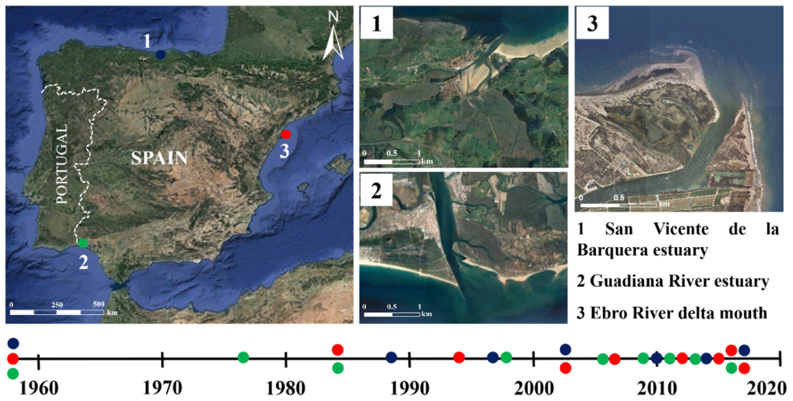
2. Study Sites
3. Materials and Methods
3.1. Estuarine Mapping and Area Calculation
3.2. Accuracy Assessment
4. Results
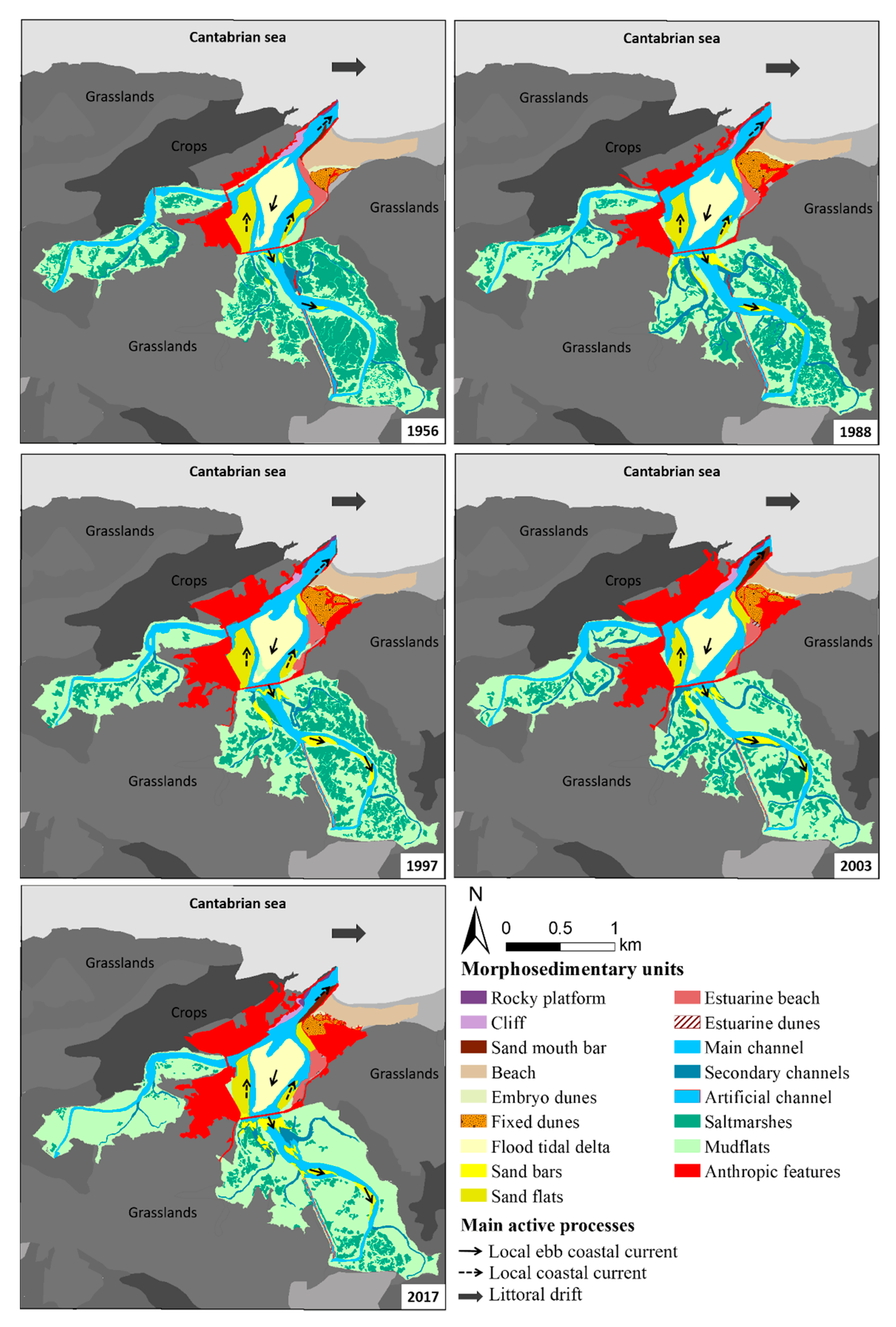
4.1. Estuarine Mapping and Area Calculation
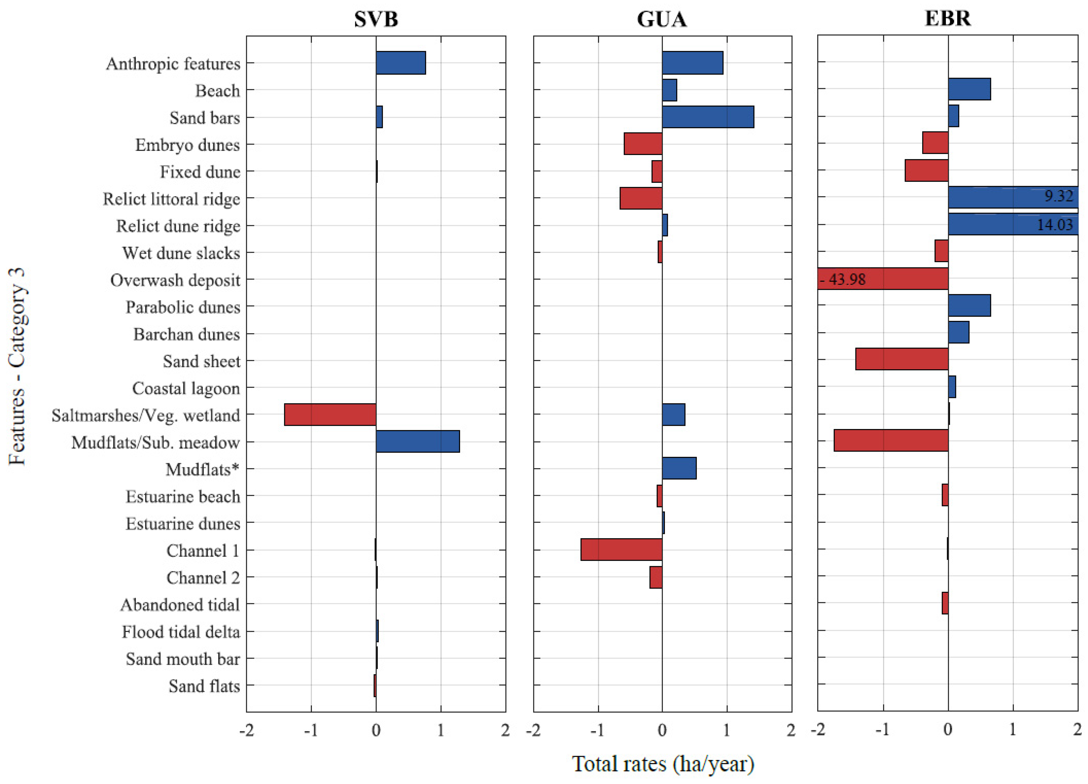
4.2. Changes in Occupied Surface
4.3. Accuracy Assessment
5. Discussion
6. Conclusions
Author Contributions
Funding
Conflicts of Interest
Appendix A

| SVB | Total Area of Each Feature (ha) along the Study Period | ||||||
|---|---|---|---|---|---|---|---|
| 1956 | 1988 | 1997 | 2003 | 2010 | 2014 | 2017 | |
| Shoreline Sandy Environments | 45.77 | 33.42 | 40.84 | 35.30 | 39.00 | 39.07 | 40.78 |
| Beach | 23.50 | 15.38 | 16.90 | 15.75 | 15.62 | 15.56 | 15.88 |
| Estuarine beach | 4.95 | 3.29 | 4.63 | 3.72 | 3.90 | 4.46 | 4.80 |
| Sand bars | 2.24 | 4.68 | 6.22 | 5.81 | 6.01 | 6.01 | 7.57 |
| Dunes | 6.04 | 11.94 | 11.38 | 10.19 | 6.37 | 6.85 | 6.17 |
| Embryo dunes | 1.57 | 1.52 | 1.08 | 1.35 | 0.60 | 0.57 | 0.87 |
| Fixed dunes | 4.47 | 10.13 | 10.13 | 8.53 | 5.53 | 6.05 | 5.09 |
| Estuarine dunes | - | 0.29 | 0.17 | 0.31 | 0.24 | 0.22 | 0.22 |
| Tidal flats | 237.86 | 223.29 | 236.86 | 228.00 | 243.55 | 244.43 | 230.03 |
| Saltmarshes | 101.70 | 50.44 | 60.01 | 43.90 | 29.68 | 26.22 | 15.62 |
| Mudflats | 136.16 | 172.85 | 176.85 | 184.10 | 213.87 | 218.21 | 214.41 |
| Drainage Network | 83.84 | 101.31 | 79.70 | 91.52 | 73.69 | 75.51 | 85.57 |
| Channel 1 | 51.30 | 62.80 | 51.20 | 51.55 | 43.96 | 44.75 | 50.44 |
| Channel 2 | 7.82 | 16.69 | 6.07 | 15.15 | 3.56 | 4.18 | 8.68 |
| Artificial channel | 2.70 | 2.17 | 1.94 | 1.61 | 1.63 | 1.63 | 1.63 |
| Sand flats | 15.08 | 10.07 | 13.09 | 10.02 | 13.47 | 13.04 | 12.53 |
| Flood tidal delta | 20.76 | 18.97 | 20.21 | 20.26 | 23.13 | 22.85 | 22.72 |
| GUA | Total Area of Each Feature (ha) along the Study Period | ||||||||
|---|---|---|---|---|---|---|---|---|---|
| 1956 | 1977 | 1984 | 1998 | 2006 | 2009 | 2011 | 2013 | 2016 | |
| Shoreline Sandy Environments | 104.23 | 68.14 | 67.14 | 200.92 | 120.58 | 55.71 | 86.76 | 138.49 | 163.22 |
| Beach | 13.65 | 16.04 | 20.96 | 22.67 | 26.38 | 22.61 | 24.26 | 31.26 | 27.15 |
| Estuarine beach | 10.11 | 9.39 | 5.27 | 8.10 | 5.60 | 3.87 | 2.78 | 3.99 | 5.22 |
| Relict littoral ridge | 65.84 | 40.33 | 37.44 | 29.23 | 29.23 | 29.23 | 26.83 | 26.83 | 26.83 |
| Coastal lagoon | - | 2.39 | 1.66 | - | 2.06 | - | 2.11 | 2.37 | 2.11 |
| Sand bars | 14.63 | 1.81 | 140.92 | 57.31 | - | 30.72 | 73.37 | 99.66 | |
| Mudflats | - | - | - | - | - | - | - | 0.67 | 2.26 |
| Dunes | 101.55 | 75.21 | 64.75 | 57.85 | 55.00 | 54.23 | 52.54 | 51.17 | 54.80 |
| Embryo dunes | 41.59 | 7.48 | 10.03 | 5.32 | 2.99 | 4.04 | 6.19 | 5.68 | 5.80 |
| Fixed dunes | 16.49 | 19.73 | 13.36 | 12.70 | 5.22 | 6.16 | 4.42 | 2.98 | 6.85 |
| Estuarine dunes | - | - | - | - | 0.13 | 0.02 | 0.22 | - | 0.46 |
| Relict dune ridge | 36.79 | 48.00 | 40.86 | 39.45 | 43.59 | 41.11 | 38.74 | 39.49 | 39.14 |
| Wet dune slacks | 6.68 | - | 0.50 | 0.38 | 3.07 | 2.90 | 2.97 | 3.03 | 2.55 |
| Tidal flats | 276.31 | 272.82 | 289.63 | 289.93 | 279.02 | 275.85 | 277.96 | 283.16 | 279.67 |
| Saltmarshes | 222.03 | 241.65 | 245.17 | 250.96 | 252.53 | 255.00 | 243.73 | 251.22 | 242.49 |
| Mudflats | 37.25 | 30.90 | 44.22 | 36.89 | 26.25 | 18.68 | 34.00 | 31.70 | 36.94 |
| Drainage Network | 377.90 | 297.97 | 291.21 | 354.75 | 331.41 | 310.99 | 318.63 | 300.64 | 290.18 |
| Channel 1 | 341.35 | 276.83 | 272.28 | 335.63 | 308.74 | 287.03 | 292.46 | 276.01 | 265.78 |
| Channel 2 | 27.20 | 15.47 | 12.48 | 12.46 | 15.25 | 15.46 | 16.46 | 15.46 | 15.54 |
| Channel 3 | 7.71 | 3.81 | 4.18 | 4.36 | 4.43 | 4.88 | 5.49 | 4.48 | 4.47 |
| EBR | Total Area of Each Feature (ha) along the Study Period | |||||||
|---|---|---|---|---|---|---|---|---|
| 1984 | 1994 | 2003 | 2007 | 2012 | 2015 | 2016 | 2017 | |
| Shoreline Sandy Environments | 99.30 | 63.12 | 55.66 | 53.81 | 86.21 | 83.88 | 86.21 | 100.72 |
| Beach | 5.83 | 22.35 | 21.77 | 20.59 | 29.16 | 24.36 | 27.18 | 27.27 |
| Estuarine beach | 4.36 | - | - | 0.18 | 0.61 | 0.76 | 0.32 | 1.40 |
| Relict littoral ridge | 15.49 | 18.95 | 25.44 | 25.69 | 23.63 | 27.95 | 26.33 | 24.81 |
| Overwash deposit | 46.89 | 18.16 | 4.77 | 4.75 | 1.69 | 4.24 | 2.32 | 2.91 |
| Coastal lagoon | - | 0.08 | 1.23 | 1.54 | 0.17 | 0.11 | - | 12.50 |
| Sand bars | 26.73 | 3.58 | 2.44 | 1.07 | 30.94 | 26.46 | 30.05 | 31.83 |
| Dunes | 104.99 | 140.11 | 109.76 | 108.36 | 103.01 | 108.04 | 111.57 | 114.32 |
| Mobile dunes | 19.83 | 39.80 | 28.56 | 23.85 | 25.33 | 31.88 | 33.10 | 43.58 |
| Embryo dunes | 19.83 | 5.04 | 2.94 | 0.43 | 1.75 | 0.27 | 4.24 | 6.79 |
| Parabolic dunes | - | - | 19.92 | 22.32 | 18.80 | 23.24 | 26.10 | 29.16 |
| Barchan dunes | - | - | 3.07 | 1.10 | - | 3.43 | 2.77 | 7.63 |
| Sand sheet | - | 34.75 | 2.64 | - | 4.79 | 4.93 | - | - |
| Fixed dunes | 21.90 | 55.97 | 3.71 | 11.19 | 4.18 | 2.74 | - | 0.19 |
| Relict dune ridge | 49.34 | 37.77 | 71.27 | 67.37 | 65.36 | 65.38 | 69.37 | 63.37 |
| Wet dune slacks | 13.91 | 6.58 | 6.22 | 5.94 | 8.13 | 8.04 | 9.10 | 7.18 |
| Wetlands | 151.12 | 121.46 | 105.97 | 111.95 | 111.71 | 105.86 | 105.36 | 106.79 |
| Vegetated wetland | - | 13.36 | 13.63 | 17.29 | 16.86 | 12.56 | 13.85 | 13.70 |
| Submerged meadow | 151.12 | 108.10 | 92.34 | 94.65 | 94.85 | 93.29 | 91.50 | 93.09 |
| Drainage Network | 93.28 | 90.43 | 90.70 | 88.59 | 83.65 | 77.44 | 83.26 | 78.20 |
| Channel 1 | 64.30 | 64.43 | 69.77 | 67.79 | 65.57 | 59.79 | 65.77 | 63.70 |
| Abandoned channel | 28.98 | 26.00 | 20.93 | 20.80 | 18.08 | 17.65 | 17.48 | 14.51 |
References
- Boerema, A.; Meire, P. Management for estuarine ecosystem services: A review. Ecol. Eng. 2017, 98, 172–182. [Google Scholar] [CrossRef]
- Davis, J.; Kidd, I.M. Identifying Major Stressors: The Essential Precursor to Restoring Cultural Ecosystem Services in a Degraded Estuary. Estuaries Coasts 2012, 35, 1007–1017. [Google Scholar] [CrossRef]
- Small, C.; Nicholls, R.J.; Summer, F.; Smallt, C. A Global Analysis of Human Settlement in Coastal Zones. J. Coast. Res. 2003, 19, 584–599. [Google Scholar] [CrossRef]
- Beaumont, N.J.; Austen, M.C.; Atkins, J.P.; Burdon, D.; Degraer, S.; Dentinho, T.P.; Derous, S.; Holm, P.; Horton, T.; van Ierland, E.; et al. Identification, definition and quantification of goods and services provided by marine biodiversity: Implications for the ecosystem approach. Mar. Pollut. Bull. 2007, 54, 253–265. [Google Scholar] [CrossRef]
- Basset, A.; Barbone, E.; Elliott, M.; Li, B.L.; Jorgensen, S.E.; Lucena-Moya, P.; Pardo, I.; Mouillot, D. A unifying approach to understanding transitional waters: Fundamental properties emerging from ecotone ecosystems. Estuar. Coast. Shelf Sci. 2013, 132, 5–16. [Google Scholar] [CrossRef]
- Atkins, J.P.; Burdon, D.; Elliott, M.; Gregory, A.J. Management of the marine environment: Integrating ecosystem services and societal benefits with the DPSIR framework in a systems approach. Mar. Pollut. Bull. 2011, 62, 215–226. [Google Scholar] [CrossRef]
- Hood, G.W. Indirect environmental effects of dikes on estuarine tidal channels: Thinking outside of the dike for habitat restoration and monitoring. Estuaries 2004, 27, 273–282. [Google Scholar] [CrossRef]
- Barbier, E.B.; Hacker, S.D.; Kennedy, C.; Koch, E.W.; Stier, A.C.; Silliman, B.R. The value of estuarine and coastal ecosystem services. Ecol. Monogr. 2011, 81, 169–193. [Google Scholar] [CrossRef]
- Grill, G.; Lehner, B.; Thieme, M.; Geenen, B.; Tickner, D.; Antonelli, F.; Babu, S.; Borrelli, P.; Cheng, L.; Crochetiere, H.; et al. Mapping the world’s free-flowing rivers. Nature 2019, 569, 215–221. [Google Scholar] [CrossRef]
- Sayers, P.B.; Hall, J.W.; Meadowcroft, I.C. Towards risk-based flood hazard management in the UK. Proc. Inst. Civ. Eng. Civ. Eng. 2002, 150, 36–42. [Google Scholar] [CrossRef]
- Ibáñez, C.; Caiola, N.; Nebra, A.; Wessels, M. Estuarios. In Bases Ecológicas Preliminares para la Conservación de los Tipos de Hábitat de Interés Comunitario en España; Ministerio de Medio Ambiente y Medio Rural y Marino: Madrid, Spain, 2009; p. 73. ISBN 978-84-491-0911-9. [Google Scholar]
- Pallero, C.; Barragán, J.M.; Scherer, M. Management international estuarine systems: The case of the Guadiana river (Spain-Portugal). Environ. Sci. Policy 2018, 80, 82–94. [Google Scholar] [CrossRef]
- Wasson, K.; Ganju, N.K.; Defne, Z.; Endris, C.; Elsey-Quirk, T.; Thorne, K.M.; Freeman, C.M.; Guntenspergen, G.; Nowacki, D.J.; Raposa, K.B. Understanding tidal marsh trajectories: Evaluation of multiple indicators of marsh persistence. Environ. Res. Lett. 2019, 14. [Google Scholar] [CrossRef]
- Chust, G.; Caballero, A.; Marcos, M.; Liria, P.; Hernández, C.; Borja, Á. Regional scenarios of sea level rise and impacts on Basque (Bay of Biscay) coastal habitats, throughout the 21st century. Estuar. Coast. Shelf Sci. 2010, 87, 113–124. [Google Scholar] [CrossRef]
- Farris, A.S.; Defne, Z.; Ganju, N.K. Identifying salt marsh shorelines from remotely sensed elevation data and imagery. Remote Sens. 2019, 11, 1795. [Google Scholar] [CrossRef]
- French, J.; Payo, A.; Murray, B.; Orford, J.; Eliot, M.; Cowell, P. Appropriate complexity for the prediction of coastal and estuarine geomorphic behaviour at decadal to centennial scales. Geomorphology 2016, 256, 3–16. [Google Scholar] [CrossRef]
- Ghosh, A. Monitoring estuarine morphodynamics through quantitative techniques and GIS: A Case study in Sagar Island, India. J. Coast. Conserv. 2019, 23, 133–148. [Google Scholar] [CrossRef]
- Laengner, M.L.; Siteur, K.; van der Wal, D. Trends in the seaward extent of saltmarshes across Europe from long-term satellite data. Remote Sens. 2019, 11, 1653. [Google Scholar] [CrossRef]
- Mury, A.; Collin, A.; Etienne, S.; Jeanson, M. Wave Attenuation Service by Intertidal Coastal Ecogeosystems in the Bay of Mont-Saint-Michel, France: Review and Meta-Analysis. In Estuaries and Coastal Zones in Times of Global Change; Nguyen, K.D., Guillou, S., Gourbesville, P., Thiébot, J., Eds.; Springer Water: Caen, France, 2020; pp. 555–572. ISBN 978-981-15-2080-8. [Google Scholar]
- Doyle, T.B.; Woodroffe, C.D. The application of LiDAR to investigate foredune morphology and vegetation. Geomorphology 2018, 303, 106–121. [Google Scholar] [CrossRef]
- Parker, K.C.; Bendix, J. Landscape-scale geomorphic influences on vegetation patterns in four environments. Phys. Geogr. 1996, 17, 113–141. [Google Scholar] [CrossRef]
- Rajakaruna, N.; Boyd, R.S. Geoecology; Oxford Bibliographies Online: Oxford, UK, 2014. [Google Scholar]
- Dalrymple, R.W.; Zaitlin, B.A.; Boyd, R. Estuarine facies models; conceptual basis and stratigraphic implications. J. Sediment. Res. 1992, 62, 1130–1146. [Google Scholar] [CrossRef]
- Woodroffe, C.D. Coasts: Form, Processes and Evolution; Cambridge University Press: Cambridge, UK, 2002. [Google Scholar]
- Castañeda, C.; Gracia, F.J.; Conesa, J.A.; Latorre, B. Geomorphological control of habitat distribution in an intermittent shallow saline lake, Gallocanta Lake, NE Spain. Sci. Total Environ. 2020, 726, 138601. [Google Scholar] [CrossRef] [PubMed]
- Schmidt, K.S.; Skidmore, A.K.; Kloosterman, E.H.; Van Oosten, H.; Kumar, L.; Janssen, J.A.M. Mapping coastal vegetation using an expert system and hyperspectral imagery. Photogramm. Eng. Remote Sens. 2004, 70, 703–715. [Google Scholar] [CrossRef]
- White, R.A.; Piraino, K.; Shortridge, A.; Arbogast, A.F. Measurement of Vegetation Change in Critical Dune Sites along the Eastern Shores of Lake Michigan from 1938 to 2014 with Object-Based Image Analysis. J. Coast Res. 2019, 35, 842–851. [Google Scholar] [CrossRef]
- Flor-Blanco, G.; Flor, G.; Pando, L.; Abanades, J. Morphodynamics, sedimentary and anthropogenic influences in the San Vicente de la Barquera estuary (North coast of Spain). Geol. Acta 2015, 13, 279–295. [Google Scholar] [CrossRef]
- Gobierno de España, Ministerio de Transportes, Movilidad y Agenda Urbana. Puertos del Estado. Available online: http://www.puertos.es/es-es/oceanografia/Paginas/portus.aspx (accessed on 22 October 2018).
- Lobo, F.J.; Plaza, F.; González, R.; Dias, J.M.A.; Kapsimalis, V.; Mendes, I.; Del Río, V.D. Estimations of bedload sediment transport in the guadiana estuary (SW Iberian Peninsula) during low river discharge periods. J. Coast. Res. 2004, 20, 12–26. [Google Scholar]
- Morales, J.A. Sedimentología del Estuario del río Guadiana. Ph.D. Thesis, Universidad de Huelva, Huelva, Spain, 1995. [Google Scholar]
- Morales, J.A.; Garel, E. The Guadiana River Delta. In The Spanish Coastal Systems: Dynamic Processes, Sediments and Management; Springer International Publishing: Cham, Switzerland, 2019; pp. 565–581. ISBN 9783319931692. [Google Scholar]
- Morales, J.A.; Pendon, G.; Borrego, J. Origen y evolución de flechas litorales recientes en la desembocadura del estuario mesomareal del río Guadiana (Huelva, SO de España). Rev. Soc. Geol. España 1994, 7, 155–167. [Google Scholar]
- Ibàñez, C.; Canicio, A.; Day, J.W.; Curcó, A. Morphologic development, relative sea level rise and sustainable management of water and sediment in the Ebre Delta, Spain. J. Coast. Conserv. 1997, 3, 191–202. [Google Scholar] [CrossRef]
- Rodríguez-Santalla, I.; Somoza, L. The Ebro River Delta. In The Spanish Coastal Systems: Dynamic Processes, Sediments and Management; Morales, J.A., Ed.; Springer Nature Switzerland: Cham, Switzerland, 2019; pp. 467–488. [Google Scholar]
- Genua-Olmedo, A. Modelling Sea Level Rise Impacts and the Management Options for Rice Production: The Ebro Delta as an Example, IRTA. Ph.D. Thesis, Universitat Rovira i Virgili, Tarragona, Spain, 2017. [Google Scholar]
- Franquet Bernis, J.M.; Albacar Damian, M.Á.; Tallada de Esteve, F. Problemática del río Ebro en su Tramo Final. Informe Acerca de los Efectos Sobre el Área Jurisdiccional de la Comunidad de Regantes—Sindicato Agrícola del Ebro, 1st ed.; UNED-Tortosa: Tortosa, Spain, 2017; ISBN 9788493842079. [Google Scholar]
- Cateura, J.; Sánchez-Arcilla, A.; Bolaños, R. Clima de viento en el delta del Ebro. Relación con el estado del mar. In El Clima entre el Mar y la Montaña; García Codron, J.C., Diego Liaño, C., de Arróyabe Hernáez, P.F., Garmendia Pedraja, C., Rasilla Álvarez, D., Eds.; University of Cantabria: Santander, Spain, 2004; pp. 463–472. [Google Scholar]
- Jiménez, J.A.; Sánchez-Arcilla, A.; Valdemoro, H.I.; Gracia, V.; Nieto, F. Processes reshaping the Ebro delta. Mar. Geol. 1997, 144, 59–79. [Google Scholar] [CrossRef]
- Martínez de Oses, F.X. Meteorología Aplicada a la Navegación, 2nd ed.; UPC, Univ. Politèc. De Catalunya: Barcelona, Spain, 2006. [Google Scholar]
- Arveti, N.; Etikala, B.; Dash, P. Land Use/Land Cover Analysis Based on Various Comprehensive Geospatial Data Sets: A Case Study from Tirupati Area, South India. Adv. Remote Sens. 2016, 5, 73–82. [Google Scholar] [CrossRef]
- National Oceanic and Atmospheric Administration. Habitat Digitizer Extension. Available online: https://coastalscience.noaa.gov/project/habitat-digitizer-extension/ (accessed on 17 June 2019).
- Zharikov, Y.; Skilleter, G.A.; Loneragan, N.R.; Taranto, T.; Cameron, B.E. Mapping and characterising subtropical estuarine landscapes using aerial photography and GIS for potential application in wildlife conservation and management. Biol. Conserv. 2005, 125, 87–100. [Google Scholar] [CrossRef]
- Stehman, S.V.; Czaplewski, R.L. Design and Analysis for Thematic Map Accuracy Assessment—An application of satellite imagery. Remote Sens. Environ. 1998, 64, 331–344. [Google Scholar] [CrossRef]
- Carter, R.W.G. Coastal Environments. An Introduction to the Physical, Ecological, and Cultural Systems of Coastlines; Academic Press: Coleraine, Northern Ireland, UK, 1988; ISBN 978-0-08-050214-4. [Google Scholar]
- Nordstrom, K.F. Estuarine Beaches: An Introduction to the Physical and Human Factors Affecting Use and Management of Beaches in estuarIes, Lagoons, Bays, and Fjords; Science, E.A., Ed.; Elsevier Science Publishers LTD: New York, NY, USA, 1992; ISBN 1851667288. [Google Scholar]
- Otvos, E.G. Beach Ridges. In Encyclopedia of Coastal Science; Finkl, C.W., Makowski, C., Eds.; Springer International Publishing: Cham, Switzerland, 2017; pp. 1–8. ISBN 978-3-319-48657-4. [Google Scholar]
- Leatherman, S.P.; Williams, A.T. Lateral Textural Grading in Overwash Sediments. Earth Surf Process. 1977, 2, 333–341. [Google Scholar] [CrossRef]
- Sanjaume, E.; Gracia, F.J. Las Dunas en España; Sanjaume, E., Gracia, F.J., Eds.; Sociedad Española de Geomorfología: Zaragoza, Spain, 2011; ISBN 9788461537808. [Google Scholar]
- Kocurek, G.; Nielson, J. Conditions favourable for the formation of warm-climate aeolian sand sheets. Sedimentology 1986, 33, 795–816. [Google Scholar] [CrossRef]
- European Commission-DG Environment. Interpretation Manual of European Union Habitats; European Environment Agency (EEA): Copenhagen, Denmark, 2007. [Google Scholar]
- Boorman, L. Salt marsh review. An overview of coastal salt marshes, theirdynamic and sensitivity characteristics for conservation and management. JNCC Rep. 2003, 1–99. [Google Scholar] [CrossRef]
- National Research Council. Wetlands: Characteristics and Boundaries; The National Academies Press: Washington, DC, USA, 1995; ISBN 978-0-309-10364-0. [Google Scholar]
- Dame, R.F. Estuaries. Encycl. Ecol. 2008, 1407–1413. [Google Scholar] [CrossRef]
- Wolanski, E.; Elliott, M.; Wolanski, E.; Elliott, M. Tidal wetlands. Estuar. Ecohydrol. 2016, 127–155. [Google Scholar] [CrossRef]
- Kjerfve, B. Coastal Lagoons. In Coastal Lagoon Processes; Kjerfve, B., Ed.; Elsevier Science Publishers: Amsterdam, The Netherlands, 1994; ISBN 0444882588. [Google Scholar]
- López-Calderón, J.M.; Meling, A.; Riosmena-Rodríguez, R. Sandflat. In Encyclopedia of Estuaries; Kennish, M.J., Ed.; Springer: Dordrecht, The Netherlands, 2016; p. 538. ISBN 978-94-017-8801-4. [Google Scholar]
- Hayes, M.O. Barrier island morphology as a function of tidal and wave regime. In Barrier Islands—From the Gulf of St. Lawrence to the Gulf of Mexico; Leatherman, S.P., Ed.; Academic Press, Inc.: London, UK, 1979; pp. 1–27. ISBN 0-12-440260-7. [Google Scholar]
- Rodríguez-Santalla, I.; Serra, J.; Montoya, I.; Sánchez, M.J. The Ebro Delta: From its origin to present uncertainty. In River Deltas: Types, Structures and Ecology; Schmidt, P.E., Ed.; Nova Science Publishers Inc.: New York, NY, USA, 2010; pp. 161–171. [Google Scholar]
- Van der Wal, D.; Wielemaker-Van den Dool, A.; Herman, P.M.J. Spatial patterns, rates and mechanisms of saltmarsh cycles (Westerschelde, The Netherlands). Estuar. Coast. Shelf Sci. 2008, 76, 357–368. [Google Scholar] [CrossRef]
- Winterwerp, J.C.; Erftemeijer, P.L.A.; Suryadiputra, N.; Van Eijk, P.; Zhang, L. Defining eco-morphodynamic requirements for rehabilitating eroding mangrove-mud coasts. Wetlands 2013, 33, 515–526. [Google Scholar] [CrossRef]
- Best, S.N.; Van der Wegen, M.; Dijkstra, J.; Willemsen, P.W.J.M.; Borsje, B.W.; Roelvink, D.J.A. Do salt marshes survive sea level rise? Modelling wave action, morphodynamics and vegetation dynamics. Environ. Model. Softw. 2018, 109, 152–166. [Google Scholar] [CrossRef]
- Chust, G.; Borja, Á.; Liria, P.; Galparsoro, I.; Marcos, M.; Caballero, A.; Castro, R. Human impacts overwhelm the effects of sea-level rise on Basque coastal habitats (N Spain) between 1954 and 2004. Estuar. Coast. Shelf Sci. 2009, 84, 453–462. [Google Scholar] [CrossRef]
- Bouma, T.J.; van Belzen, J.; Balke, T.; van Dalen, J.; Klaassen, P.; Hartog, A.M.; Callaghan, D.P.; Hu, Z.; Stive, M.J.F.; Temmerman, S.; et al. Short-term mudflat dynamics drive long-term cyclic salt marsh dynamics. Limnol. Oceanogr. 2016, 61, 2261–2275. [Google Scholar] [CrossRef]
- van de Koppel, J.; van der Wal, D.; Bakker, J.P.; Herman, P.M.J. Self-organization and vegetation collapse in salt marsh ecosystems. Am. Nat. 2005, 165. [Google Scholar] [CrossRef]
- Fagherazzi, S.; Kirwan, M.L.; Mudd, S.M.; Guntenspergen, G.R.; Temmerman, S.; D’Alpaos, A.; van de Koppel, J.; Rybczyk, J.M.; Reyes, E.; Craft, C.; et al. Numerical models of salt marsh evolution: Ecological, Geomorphic, and Climatic Factors. Rev. Geophys. 2012, 50, 28. [Google Scholar] [CrossRef]
- Leonardi, N.; Ganju, N.K.; Fagherazzi, S. A linear relationship between wave power and erosion determines salt-marsh resilience to violent storms and hurricanes. Proc. Natl. Acad. Sci. USA 2016, 113, 64–68. [Google Scholar] [CrossRef]
- Ganju, N.K.; Defne, Z.; Kirwan, M.L.; Fagherazzi, S.; D’Alpaos, A.; Carniello, L. Spatially integrative metrics reveal hidden vulnerability of microtidal salt marshes. Nat. Commun. 2017, 8. [Google Scholar] [CrossRef]
- Garel, E.; Sousa, C.; Ferreira, Ó.; Morales, J.A. Decadal morphological response of an ebb-tidal delta and down-drift beach to artificial breaching and inlet stabilisation. Geomorphology 2014, 216, 13–25. [Google Scholar] [CrossRef]
- Talavera, L.; Del Río, L.; Benavente, J. UAS-based high-resolution record of the response of a seminatural sandy spit to a severe storm. J. Coast. Res. 2020, in press. [Google Scholar] [CrossRef]
- Wong, P.P.; Losada, I.J.; Gattuso, J.-P.; Hinkel, J.; Khattabi, A.; McInnes, K.; Saito, Y.; Sallenger, A. Coastal Systems and Low-Lying Areas. In Climate Change 2014: Impacts, Adaptation, and Vulnerability. Part A: Global and Sectoral Aspects. Contribution of Working Group II to the Fifth Assessment Report of the Intergovernmental Panel on Climate Change; Field, C.B., Barros, V.R., Dokken, D.J., Mach, K.J., Mastrandrea, M.D., Bilir, T.E., Chatterjee, M., Ebi, K.L., Estrada, Y.O., Genova, R.C., et al., Eds.; Cambridge University Press: Cambridge, UK; New York, NY, USA, 2014; pp. 361–409. ISBN 978-1107641655. [Google Scholar]
- Church, J.A.; Clark, P.U. Sea level change. In Climate Change 2013: The Physical Science Basis. Contribution of Working Group I to the Fifth Assessment Report of the Intergovernmental Panel of Climate Change; Stocker, T.F., Qin, D., Plattner, G.-K., Tignor, M., Allen, S.K., Boschung, J., Nauels, A., Xia, Y., And, V.B., Midgley, P.M., Eds.; Cambridge University Press: Cambridge, UK; New York, NY, USA, 2013; pp. 1137–1216. ISBN 9780128130810. [Google Scholar]
- Ciscar, J.C.; Iglesias, A.; Feyen, L.; Szabó, L.; Van Regemorter, D.; Amelung, B.; Nicholls, R.; Watkiss, P.; Christensen, O.B.; Dankers, R.; et al. Physical and economic consequences of climate change in Europe. Proc. Natl. Acad. Sci. USA 2011, 108, 2678–2683. [Google Scholar] [CrossRef]
- Cendrero, A.; Sánchez-Arcilla, A.; Zazo, C. Impactos sobre las zonas costeras. In Evaluación Preliminar de los Impactos en España por Efecto del Cambio Climático; Ministerio de Medio Ambiente: Madrid, Spain, 2005; pp. 469–524. ISBN 8483203030. [Google Scholar]
- Vousdoukas, M.I.; Ranasinghe, R.; Mentaschi, L.; Plomaritis, T.A.; Athanasiou, P.; Luijendijk, A.; Feyen, L. Sandy coastlines under threat of erosion. Nat. Clim. Chang. 2020, 10, 260–263. [Google Scholar] [CrossRef]
- Wolanski, E. Bounded and unbounded boundaries—Untangling mechanisms for estuarine-marine ecological connectivity: Scales of m to 10,000 km—A review. Estuar. Coast. Shelf Sci. 2017, 198, 378–392. [Google Scholar] [CrossRef]
- Wolanski, E.; Elliott, M. (Eds.) Estuarine ecological structure and functioning. In Estuarine Ecohydrology; Elsevier Science: Amsterdam, The Netherlands, 2015; pp. 157–193. ISBN 9780444633989. [Google Scholar]
- Wolanski, E.; Elliott, M. (Eds.) Estuarine water circulation. In Estuarine Ecohydrology; Elsevier Science: Amsterdam, The Netherlands, 2015; pp. 35–76. ISBN 9780444633989. [Google Scholar]
- Talavera, L. UAS-Based Monitoring of Sandy Coasts in the Bay of Cádiz (SW Spain). Ph.D. Thesis, University of Cádiz, Cádiz, Spain.
- Sturdivant, E.J.; Lentz, E.E.; Thieler, E.R.; Farris, A.S.; Weber, K.M.; Remsen, D.P.; Miner, S.; Henderson, R.E. UAS-SfM for coastal research: Geomorphic feature extraction and land cover classification from high-resolution elevation and optical imagery. Remote Sens. 2017, 9, 1020. [Google Scholar] [CrossRef]
- Olofsson, P.; Foody, G.M.; Herold, M.; Stehman, S.V.; Woodcock, C.E.; Wulder, M.A. Good practices for estimating area and assessing accuracy of land change. Remote Sens. Environ. 2014, 148, 42–57. [Google Scholar] [CrossRef]


| Feature | Description, Eco-Geomorphological Role |
|---|---|
| Shoreline Sandy Environments (1): gently sloping sand-covered shorelines affected by waves and current actions, just above the normal tide limit (EUNIS classification). | |
| Beach (2) | Accumulation of shore material formed into distinctive shapes by waves and currents. The beach form is generally a seaward-sloping boundary between a water body and mobile sediment, and a flat or landward-sloping surface at the upper limit of the beach [45]. |
| Estuarine beach (2) | Unvegetated or partially vegetated, sand, gravel, or shell intertidal beach in partially enclosed areas (estuaries, bays, lagoons and similar features) connected to the ocean dynamics [46]. |
| Relict littoral ridge (2) | Non-active often wind-constructed shore-ridge, generally parallel to the coastline with landward-adjacent similar ridges [47]. |
| Overwash deposit (2) | The continuation of the uprush over the crest of the most landward (storm) berm. The resulting deposit is not subject to reworking on the active beach by normal wave and tidal action [48]. |
| Sand bar (2) | Intertidal ridge-shaped accumulations of sand with an associated horn landward. It can be bare, without associated vegetation, or present seagrasses and algae. |
| Dunes (1): Sandy accumulations generated by wind dynamics that develop behind beaches with enough sediment availability [49] | |
| Mobile dunes (2) | Primary dunes without vegetation or with only a few species of dune-building plants [49]. They are colonized by pioneer vegetation typical of the first dune ridge (Ammophila arenaria, Elymus farctus, Euphorbia paralias, Pancratium maritimum, Calystegia soldanella, Polygonum maritimum, among others). |
| Embryo dunes (3) | The most elemental and smaller dune formations [49]. |
| Parabolic dunes (3) | U-shaped dunes with convex noses trailed by elongated arms [49]. |
| Barchan dunes (3) | A crescent-shaped dune, downwind orientated [49]. |
| Sand sheets (3) | Areas of aeolian sand where dunes with slip faces are generally absent [50]. |
| Fixed dunes (2) | Aeolian deposits whose mobility is impeded by a consistent plant cover (shrub or tree nature). Typical species of this band of the dune system are Crucianella maritima, Helicrysum stoechas, Sporobolus arenarius and Armeria spp., among others. |
| Estuarine dunes (2) | Accumulations of sand, gravel, or shell on the back part of estuarine beaches in partially enclosed areas (estuaries, bays, lagoons and similar features) connected to the ocean dynamics. They present the same species as external dunes and, exceptionally, halophytes typical of tidal environments (e.g., Sarcocornia spp. and Arthrocnemun spp.) |
| Relict dune ridges (2) | Non-active dune ridges formed by aeolian processes, usually from fine-to-medium sand, by accretion of embryonic backshore/berm dunes behind the high tide zone [47]. The associated vegetation is typical of mature and established soils, i.e., tree and shrub vegetation. |
| Wet dune slacks (2) | Damp or wet hollows left between dunes where the groundwater reaches or approaches the surface of the sand [51]. Rushes and wet grasses are the main plant communities present in these features. |
| Tidal flats1 (1): Sedimentary plains developed in areas affected by tides, with a predominance of fine sediment transported by water and stabilized by vegetation [52]. Wetlands2 (1): Shallow aquatic environments, from brackish to hypersaline, isolated or partially connected to the sea in environments with low tidal ranges. | |
| 1 Saltmarshes/2 Vegetated wetlands (2) | 1 Coastal ecosystem in the upper coastal intertidal zone between land and open saltwater or brackish water, which are intermittently flooded by the tides and colonized by halophytes. 2 Wetlands are ecosystems that depend on constant or recurrent shallow inundation or saturation at or near the surface of the substrate. Common diagnostic features of wetlands are hydric soils and hydrophytic vegetation [53]. |
| 1 Mudflats/2 Submerged meadows (2) | 1 Muddy platforms common to the intertidal zone of most estuaries (zone below neap high-tide level). The vegetation of these features is poor, mainly seagrasses and pioneer saltmarsh plants [54]. 2 Permanent shallow-flooded wetlands by seawater, colonized by salt-tolerant species [55]. |
| Coastal lagoon (2) | Inland water body, usually oriented parallel to the coast, separated from the ocean by a barrier, connected to the ocean by one or more restricted inlets, and having depths which seldom exceed a couple of meters [56]. |
| Drainage Network (1): Estuarine channel system, including minor forms related to their bottom and margins. | |
| Channel 1 (2) | Main river channel. It is the estuary in the strict sense, which extends upstream to the edge of the salt wedge [31]. |
| Channel 2 (2) | Distributary channels directly derived from the main channel. |
| Channel 3 (2) | Distributary channels derived from the secondary distributary channels. |
| Artificial channel (2) | Non-natural channels within the fluvial network. |
| Sand flat (2) | Sandy environment located preferentially in the lower intertidal zone. It is an unstable area characterized by the constant resuspension of sediment by tidal flood and ebb currents [57]. |
| Flood tidal delta (2) | Accumulation of sand on the shoreward side of an inlet, initially formed during storm surges and maintained by flood currents [58]. |
| Ebb tidal delta (2) | Accumulation of sand on the seaward side of an inlet formed by the ebb tidal current [58]. |
| Rocky units (1): Bedrock, boulders and cobbles which occur in the intertidal zone (EUNIS classification). | |
| Cliff (2) | Very steep, vertical, or overhanging rock slopes |
| Rocky platform (2) | Flat (planar) platforms carved into rocks formed by weathering and wave erosive action. |
| Map/Reference | (1) | (2) | (3) | (4) | (5) | (6) | (7) | (8) | (9) | (10) | (11) | |
|---|---|---|---|---|---|---|---|---|---|---|---|---|
| Anthropic Features (1) | 10.0 | 0.0 | 0.0 | 0.0 | 0.0 | 0.0 | 0.0 | 0.0 | 0.0 | 0.0 | 0.0 | 100.0 |
| Beach (2) | 0.0 | 13.0 | 6.0 | 0.0 | 0.0 | 0.0 | 0.0 | 0.0 | 0.0 | 0.0 | 0.0 | 68.4 |
| Embryo Dunes (3) | 0.0 | 0.0 | 4.0 | 0.0 | 0.0 | 2.0 | 0.0 | 0.0 | 0.0 | 0.0 | 0.0 | 66.7 |
| Estuarine Beaches (4) | 0.0 | 0.0 | 0.0 | 10.0 | 2.0 | 0.0 | 0.0 | 0.0 | 0.0 | 0.0 | 0.0 | 0.0 |
| Estuarine Dunes (5) | 0.0 | 0.0 | 0.0 | 1.0 | 5.0 | 0.0 | 0.0 | 0.0 | 0.0 | 0.0 | 0.0 | 0.0 |
| Fixed Dunes (6) | 0.0 | 0.0 | 0.0 | 0.0 | 0.0 | 8.0 | 0.0 | 0.0 | 0.0 | 0.0 | 0.0 | 0.0 |
| Flood Tidal Delta (7) | 0.0 | 0.0 | 0.0 | 0.0 | 0.0 | 0.0 | 10.0 | 0.0 | 0.0 | 0.0 | 0.0 | 0.0 |
| Mudflats (8) | 0.0 | 0.0 | 0.0 | 0.0 | 0.0 | 0.0 | 0.0 | 23.0 | 4.0 | 0.0 | 0.0 | 0.0 |
| Saltmarshes (9) | 0.0 | 0.0 | 0.0 | 0.0 | 0.0 | 0.0 | 0.0 | 0.0 | 13.0 | 0.0 | 0.0 | 0.0 |
| Sand Bars (10) | 0.0 | 0.0 | 0.0 | 0.0 | 0.0 | 0.0 | 0.0 | 2.0 | 0.0 | 6.0 | 0.0 | 0.0 |
| San Flats (11) | 0.0 | 0.0 | 0.0 | 0.0 | 0.0 | 0.0 | 0.0 | 0.0 | 0.0 | 0.0 | 10.0 | 0.0 |
| 100.0 | 100.0 | 40.0 | 90.9 | 71.4 | 80.0 | 100.0 | 92.0 | 76.5 | 100.0 | 100.0 |
© 2020 by the authors. Licensee MDPI, Basel, Switzerland. This article is an open access article distributed under the terms and conditions of the Creative Commons Attribution (CC BY) license (http://creativecommons.org/licenses/by/4.0/).
Share and Cite
Aranda, M.; Gracia, F.J.; Peralta, G. Estuarine Mapping and Eco-Geomorphological Characterization for Potential Application in Conservation and Management: Three Study Cases along the Iberian Coast. Appl. Sci. 2020, 10, 4429. https://doi.org/10.3390/app10134429
Aranda M, Gracia FJ, Peralta G. Estuarine Mapping and Eco-Geomorphological Characterization for Potential Application in Conservation and Management: Three Study Cases along the Iberian Coast. Applied Sciences. 2020; 10(13):4429. https://doi.org/10.3390/app10134429
Chicago/Turabian StyleAranda, María, Francisco Javier Gracia, and Gloria Peralta. 2020. "Estuarine Mapping and Eco-Geomorphological Characterization for Potential Application in Conservation and Management: Three Study Cases along the Iberian Coast" Applied Sciences 10, no. 13: 4429. https://doi.org/10.3390/app10134429
APA StyleAranda, M., Gracia, F. J., & Peralta, G. (2020). Estuarine Mapping and Eco-Geomorphological Characterization for Potential Application in Conservation and Management: Three Study Cases along the Iberian Coast. Applied Sciences, 10(13), 4429. https://doi.org/10.3390/app10134429