On the Influence of Suspension Geometry on Steering Feedback

Abstract

Feedback through the steering wheel is known as the most important source of information to the driver. The so-called steering feeling, composed of self-aligning actions coming from tyres and suspension geometry all the way through mechanical linkages to the driver’s hands, provides vital communication for intuitive driving, and it is therefore utterly important for safety and for a pleasant driving experience as well. Subtle forces and vibrations, due to the interaction between the tyre contact patch and the road surface texture, also play a role, provided they are not heavily filtered or cancelled by the power steering system. Human perception is guided by experience in order to establish correlations between steering feedback and vehicle motion in terms of straight-line stability, cornering speed, tyre adhesion and available friction, vehicle balance, and so on. A front-wheel drive car is potentially a critical vehicle from this point of view, especially when the powertrain can deliver large torque figures, and even more so if a limited-slip differential (LSD) or a similar active device is present in order to improve traction capabilities. Any difference between the two wheels in terms of tractive force can result into the so-called torque steer issue, that is to say, a “pulling” sensation on the steering wheel or a shifting of the vehicle from the desired trajectory. This paper analyses the torque steer phenomenon on an all-wheel-drive, full electric sportscar where a significant portion of the torque is transferred to the front axle. The effects of suspension kinematics and the load variation at tyre contact patch level are taken into account. For evaluating the impact of steering feedback, the VI-grade^® simulation software is adopted and a test campaign on the professional driving simulator available at the University of Brescia has been carried out in order to understand the impact of steering feedback on driver perception and performance.

1. Introduction

As stated by the authors in [1,2], the steering system and geometry have a primary impact on the tactile feel perceived by the driver through his hands acting on the steering wheel. This perception —often called “steering feel”— is considered to be vital because steering is the driver’s main line of communication with the car; distortion in this guidance channel makes every other perception more difficult to comprehend [3]. Friction in the steering line, for instance, must be accurately calibrated in order to prevent stick and slip effects that could heavily affect returnability and the on-centre feel, while providing enough damping at the same time [2]. According to [4], steering feel or steering torque feedback is widely regarded as an important aspect of the handling quality of a vehicle, as it is known to help the driver in reducing path-following errors. Some authors even suggest that, apart from eyesight, the driving action is mainly based on feedback communication through the steering system [5]. Therefore, any interaction between the steering system on one side, and the effects of power delivery, braking torque, load transfer and road surface irregularities on the other, should be very carefully handled in order not to alter such a vital feedback. The disturbance related to unequal braking forces on the two sides is called “brake pull”, while the disturbance induced by uneven tractive forces on the front axle is known as “torque steer” [6,7]. They are both undesirable because they upset the correlation between lateral acceleration (hence cornering speed), steering angle and steering effort.

Standard front-wheel drive (FWD) cars are normally equipped with a so-called open or free differential delivering torque in equal amounts to the wheels on both sides. Therefore, torque steer effects can be a consequence of rarely found non-symmetrical designs between the left and right half-shaft geometry, such as different shaft length, rotational inertia and inclination angle [8]. Transient phenomena like powertrain movements over elastic mountings and large roll angles also play a role, while minor effects can be due to suspension geometry tolerances, tyre conicity and wear and asymmetric mass distribution as a consequence of vehicle loading [9]. Finally, whenever occasional wheelspin occurs under heavy acceleration, inertia effects can also induce unpleasant self-steering transients.

Where present, a limited-slip differential (LSD) can help to mitigate traction problems in cars featuring a high torque-to-weight ratio or on low-friction surfaces. The LSD can also be tuned to improve handling and stability by generating a yaw moment influencing the handling characteristics [10,11,12,13]. 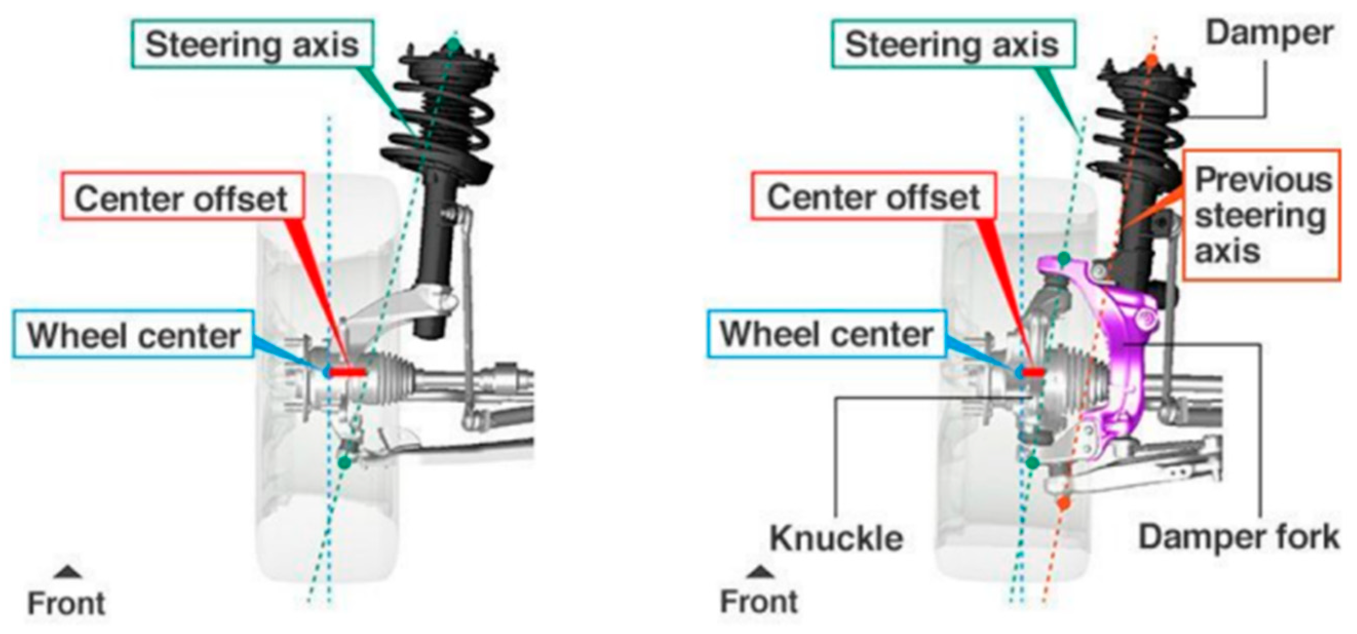However, relevant torque steer problems were encountered when limited-slip differentials first appeared in front-wheel drive rally cars in the early 1970s, given the large asymmetry in terms of torque and tractive force generated under certain conditions [14,15]. Peculiar geometries have been designed with the aim of minimising these effects. For example, the McPherson suspension with separate steering axis found in sporty Honda cars (see Figure 1) is aimed at reducing the wheel center arm (KO, see chapter 2). The very same concept can be found on the so-called RevoKnuckle^® Ford geometry [16].

It should also be stated that it is not possible to eliminate the asymmetry of driving or braking torque applications completely. As a matter of fact, the resultant forces exchanged between the tyre and the ground can move laterally across the contact patch, especially on uneven road surfaces and with wide tyres, thus inducing torque steer or brake pull [6].

High-performance or special application vehicles can feature active differentials or torque vectoring devices aimed at extending the performance and stability envelopes by further enhancing yaw motion control [17,18,19,20,21,22,23,24,25,26,27,28]. Where a passive LSD or these advanced devices are adopted on the front axle, the control of torque steer phenomena should be taken into account from the very early design stages. Electric power-assisted steering (EPAS) systems also offer the opportunity to cancel out torque steer by means of suitable control strategies [29]

It is, however, where the torque can be controlled independently on each wheel that the torque vectoring concept can be taken to new heights [30]. On electric vehicles with a multiple-motor powertrain, for instance, the torque vectoring can be achieved with individual wheel torque control. This feature can significantly enhance the cornering response, driving stability, performance and active safety whilst improving vehicle dynamic properties and/or the fun-to-drive attitude of the car. Torque vectoring can also increase energy efficiency through the appropriate design of the reference understeer characteristics and the calculation of the wheel torque distribution providing either the desired total wheel torque and a direct yaw moment [31,32,33].

Today, the evolution of the automotive world towards electrification means that a variety of hybrid and electric cars with different powertrain/transmission architectures can be found on the market. In the specific case of an electric or hybrid car, one or two independent electric motors can be installed on a driving axle. Therefore, it is possible to use the control system of these motors to deliver different torques to the left and right wheel. A front driving axle with independent motors therefore raises the bar of the torque steer challenge. Furthermore, in the case of an electric powertrain, the very fast response times related to a driver input could generate sudden torque peaks on the steering wheel, thus making feedback even worse than traditional FWD cars equipped with an LSD or an actively controlled differential.

This paper is aimed at providing an insight on the torque steer phenomenon in light of the shift towards full electric vehicles even in the high-performance market segment, in order to understand which geometric parameters of the car it is directly connected to, starting with a comprehensive theoretical background.

Examples of suspension kinematic re-design are proposed to minimise the torque steer effects with the help of a specific software. Such a tool has been self-developed within the Automotive Engineering Group of Brescia University by the authors of this work. The development process is reported in [34]. A thorough validation was carried out by comparing results with commercial tools, like Lotus Suspension Design (Shark^®) by Lotus Engineering and with the Adams multi-body package. This proprietary tool:

• enables the design and analysis of all kinds of suspension geometries (from swing arm to full multi-link to typical racecar layouts), including kinematics of the complete steering line;
• allows any kind of user to quickly perform a ground-up design;
• can plot all the relevant suspension characteristics;
• can overlay results coming from incremental design steps;
• features a specific setup mode to simulate the effects of suspension adjustability;
• features the direct export of suspension kinematics towards professional simulation packages like CarSim^® and VI-CarRealTime^®;
• has been successfully employed in some previous works [35,36].

Finally, a simulation campaign is carried out on VI-grade’s VI-CarRealTime^® (VI-CRT) simulation environment with standard sine steer and track laps. The results will be reported.

2. Materials and Methods

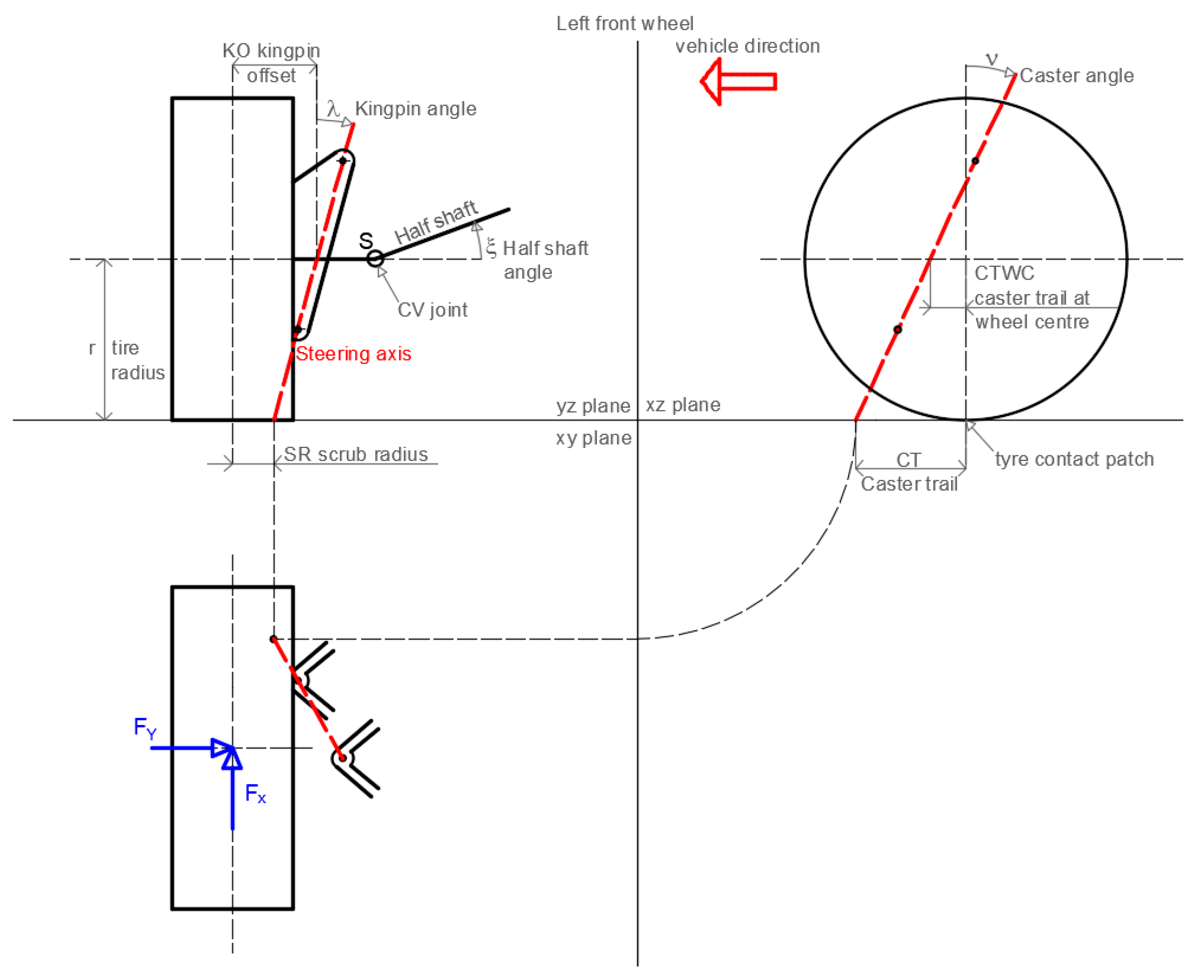
First, the torque steer theory has been analysed with particular focus on the geometric parameters. The main steering geometry parameters are defined in Figure 2.

In particular, the scrub radius (SR) is defined as the distance between the tyre contact patch mid-point and the intersection between the steering axis and the road surface projected onto the yz plane, the caster trail (CT) is the same distance projected onto the xz plane and the wheel center arm or kingpin offset (KO) is the distance between the steering axis and the wheel center, projected onto the horizontal plane (see top left of Figure 2).

A simple case of driving along a straight line at constant speed is taken as a reference. Considering the front left wheel and analysing the equilibrium around the spindle point S, a few simplified configurations will be used to explain the balance of forces and moments acting on the front wheel assembly.

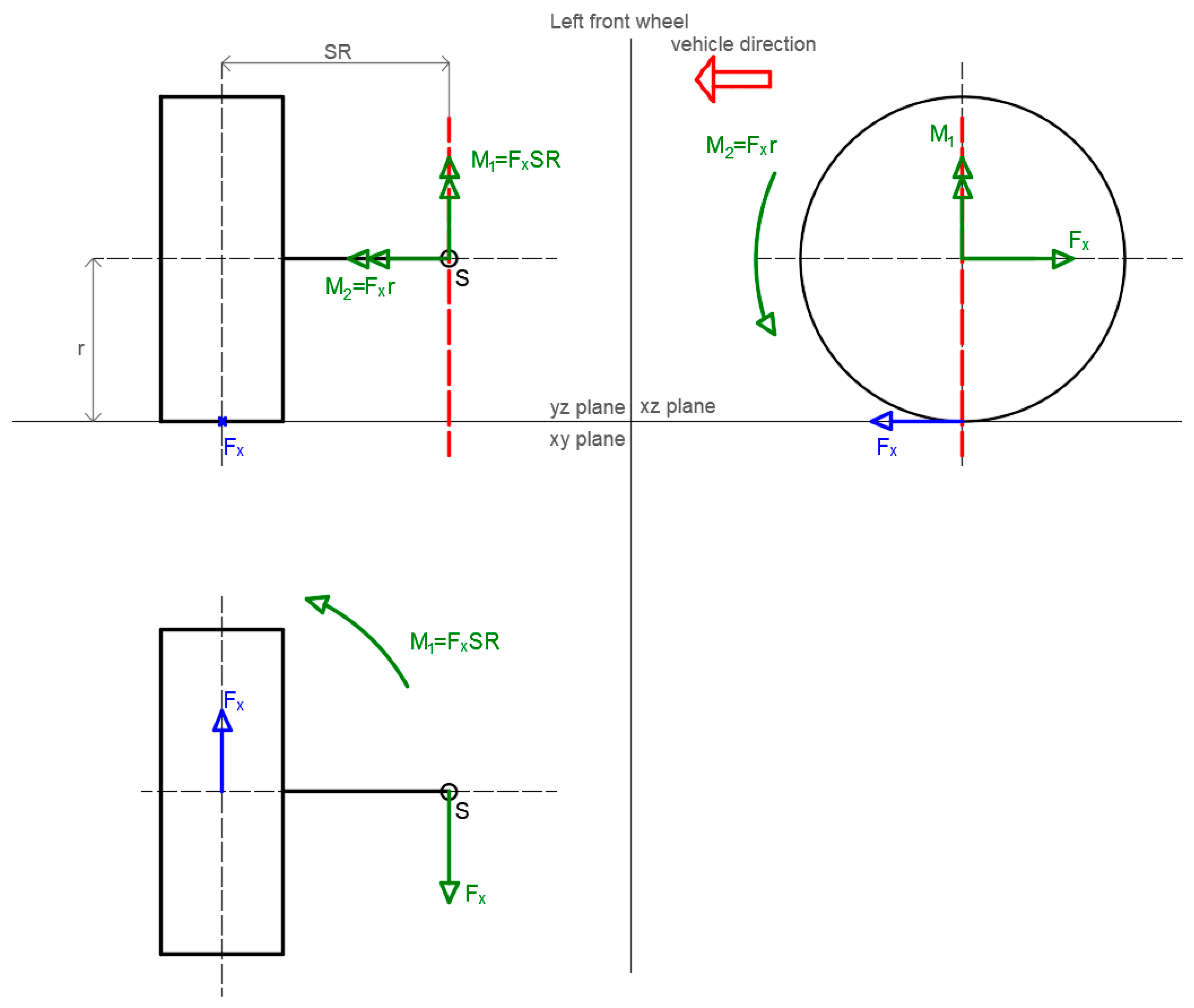
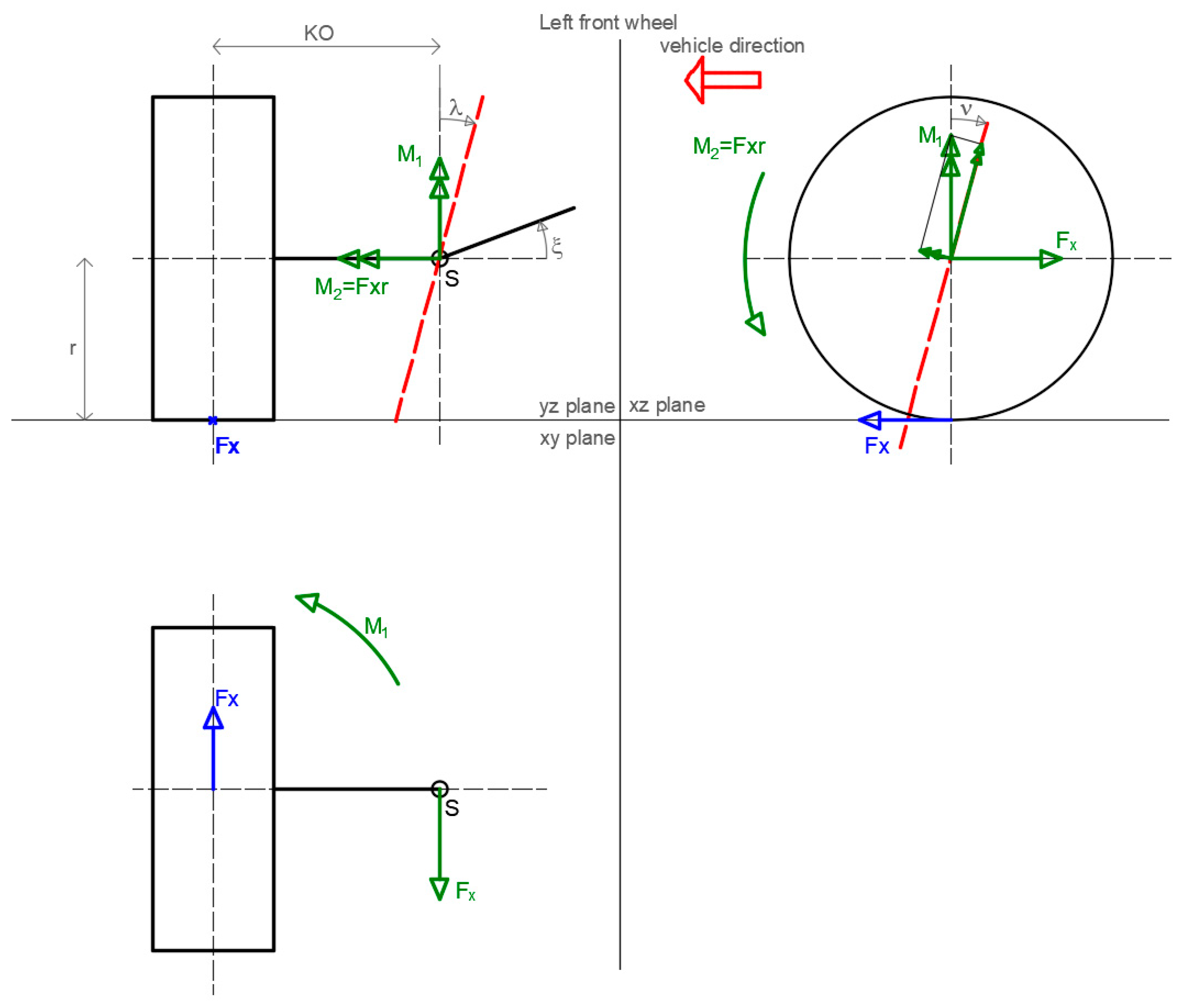
2.1. Case 1

The first simplified case considers a vertical steering axis passing through point S and a half shaft aligned along the Y-axis (Figure 3). The longitudinal force driving the vehicle under power is Fx. In order to consider it as applied at the tyre contact patch, a balance force must be applied at S, thus generating moments M₁ and M₂, while the vertical load is balanced through the spring unit, and as such, it is not relevant.

The reaction forces are:

∑F(axis x) = Fx − Rx = 0 ⇒ Rx = Fx

(1)

∑F(axis y), F(axis z) = 0

(2)

∑Mxy (S) = −Fx∙SR +M₁ ⇒ M₁ = Fx∙SR

(3)

∑Mxz (S) = −Fx∙r + M₂ ⇒ M₂ = Fx∙r

(4)

Since the steering axis is vertical, the only component of the moment responsible for the torque steer is proportional to the scrub radius.

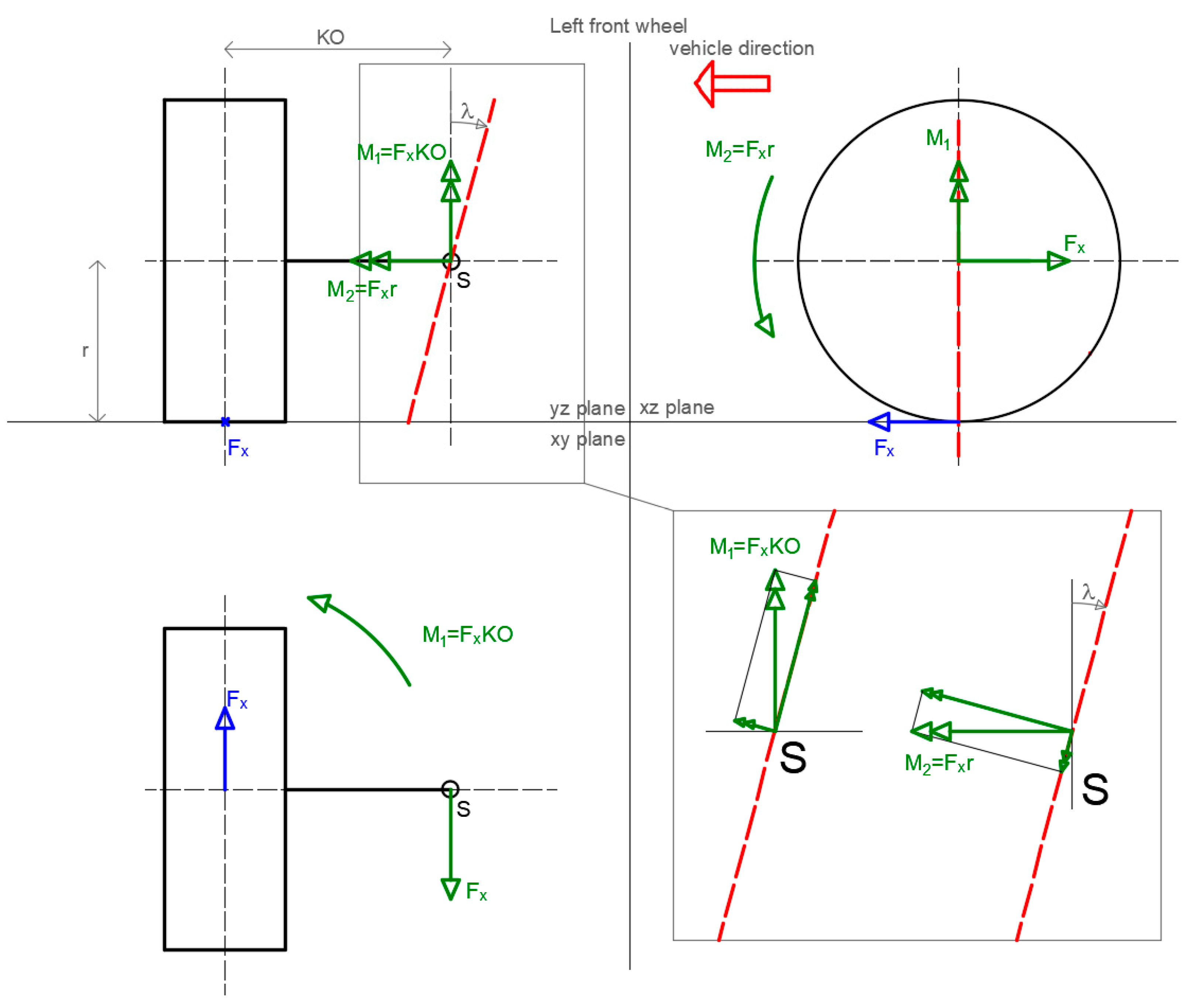
2.2. Case 2

In the second case, the steering axis is inclined by the so-called kingpin angle λ, while the half shaft is still horizontal and transverse (Figure 4).

The arm at wheel center height is:

KO = SR + r∙tan(λ)

(5)

With a non-zero kingpin angle, the moment components around the steering axis are:

M_1∥ = M₁∙cos(λ) = Fx∙KO∙cos(λ)

(6)

M_2∥ = M₂∙sin(λ) = −Fx∙r∙sin(λ)

(7)

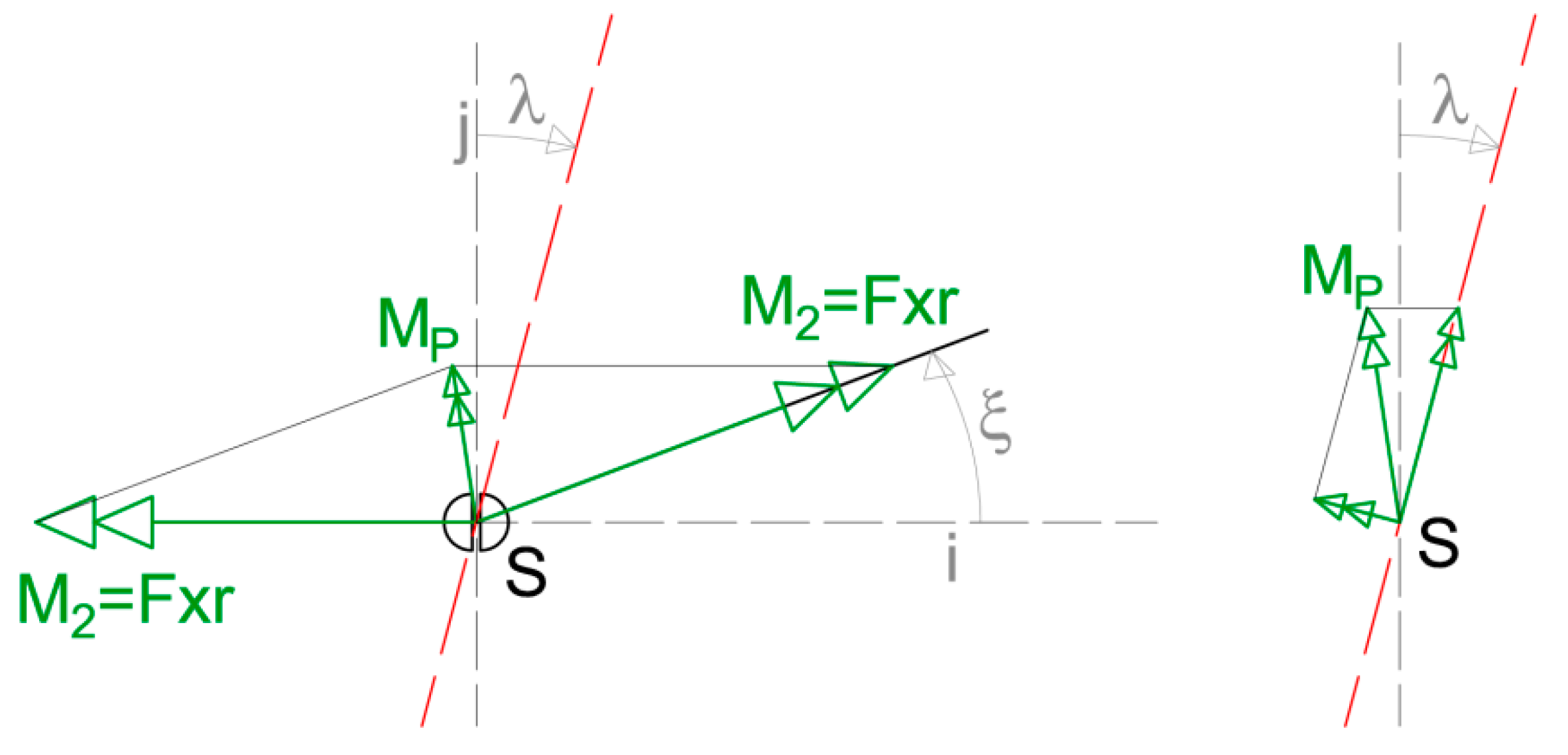
2.3. Case 3

The third case introduces the half-shaft inclination ξ in the transverse plane (Figure 5):

In a FWD car with an independent suspension system, the differential output is not necessarily aligned with the wheel axis. In any case, it is usually connected to the spindle by means of a half shaft (or driveshaft) and two constant velocity (CV) joints, with an inclination angle ξ. Given the nature of the CV joints, the driving torque remains constant along the half shaft. A secondary torque (Mp, Figure 6) is established as a function of the angle of inclination of the axle half shaft ξ.

With reference to the S point, the power balance is:

M₂∙ω_hub = C_m∙ω_m

(8)

where ω_hub is the angular velocity at the wheel hub and ω_m and C_m are the angular velocity and output torque at the differential.

And again, due to the nature of the CV joint:

ω_m = ω_hub

(9)

So:

M₂ = C_m

(10)

The vector notation is used in order to establish the entity of Mp, which is the vector sum of M₂ on the two sides of the joint:

$$\overrightarrow{\mathrm{M}\mathrm{p}}=-{\mathrm{M}}_2\overrightarrow{\mathrm{i}}+{\mathrm{M}}_2·\mathrm{c}\mathrm{o}\mathrm{s}(\mathsf{\xi })\overrightarrow{\mathrm{i}}+{\mathrm{M}}_2·\mathrm{s}\mathrm{i}\mathrm{n}(\mathsf{\xi })\overrightarrow{\mathrm{j}}={\mathrm{M}}_2·[\mathrm{c}\mathrm{o}\mathrm{s}(\mathsf{\xi })-1]\overrightarrow{\mathrm{i}}+{\mathrm{M}}_2·\mathrm{s}\mathrm{i}\mathrm{n}(\mathsf{\xi })\overrightarrow{\mathrm{j}}$$

(11)

The module is:

$$\left|\mathrm{M}\mathrm{p}\right|=\sqrt{{\mathrm{M}}_2{}^2[\mathrm{c}\mathrm{o}{\mathrm{s}}^2\left(\mathsf{\xi }\right)+1-2\mathrm{c}\mathrm{o}\mathrm{s}(\mathsf{\xi })]+{\mathrm{M}}_2{}^2\mathrm{s}\mathrm{i}\mathrm{n}(\mathsf{\xi })}={\mathrm{M}}_2\sqrt{2[1-\mathrm{c}\mathrm{o}\mathrm{s}(\mathsf{\xi })]}$$

(12)

Now, the secondary component Mp is projected on the steering axis, which is inclined by an angle λ, and as such it is identified by the unit vector:

$$\overrightarrow{\mathrm{u}}=\mathrm{s}\mathrm{i}\mathrm{n}(\mathsf{\lambda })\overrightarrow{\mathrm{i}}+\mathrm{c}\mathrm{o}\mathrm{s}(\mathsf{\lambda })\overrightarrow{\mathrm{j}}$$

(13)

The scalar product is:

$$\overrightarrow{\mathrm{M}\mathrm{p}\mathrm{u}}=\overrightarrow{\mathrm{M}\mathrm{p}}·\overrightarrow{\mathrm{u}}={\mathrm{M}}_2·\mathrm{s}\mathrm{i}\mathrm{n}(\mathsf{\lambda })·[\mathrm{c}\mathrm{o}\mathrm{s}(\mathsf{\xi })-1]\overrightarrow{\mathrm{i}}+{\mathrm{M}}_2·\mathrm{c}\mathrm{o}\mathrm{s}(\mathsf{\lambda })\mathrm{s}\mathrm{i}\mathrm{n}(\mathsf{\xi })\overrightarrow{\mathrm{j}}$$

(14)

$$\left|\mathrm{M}\mathrm{p}\mathrm{u}\right|={\mathrm{M}}_2\sqrt{\mathrm{s}\mathrm{i}{\mathrm{n}}^2(\mathsf{\lambda })\mathrm{c}\mathrm{o}{\mathrm{s}}^2(\mathsf{\xi })+1-2\mathrm{c}\mathrm{o}\mathrm{s}(\mathsf{\xi })+\mathrm{c}\mathrm{o}{\mathrm{s}}^2\left(\mathsf{\lambda }\right)\mathrm{s}\mathrm{i}\mathrm{n}(\mathsf{\xi })}$$

(15)

2.4. Case 4

The fourth and last case features the same configuration as case 3. However, the caster angle on plane xz is now non-zero (Figure 7).

The equations are the same as case 3, but the M₁ component in the xz plane now changes to:

M_1c = M₁∙cos(ν) = Fx∙KO∙cos(ν)

(16)

On the xy plane:

M_1|| = M_1c∙cos(λ) = Fx∙KO∙cos(ν)cos(λ)

(17)

Then the torque module on the steering axis is:

$$\begin{array}{c}\left|\mathrm{M}\mathrm{S}\mathrm{A}\right|=\left|\mathrm{M}{1}_{\parallel }|+|\mathrm{M}\mathrm{p}\mathrm{u}\right|\\ =\mathrm{F}\mathrm{x}\text{ [}\mathrm{K}\mathrm{O}·\mathrm{c}\mathrm{o}\mathrm{s}\left(\mathsf{\nu }\right)\mathrm{c}\mathrm{o}\mathrm{s}\left(\mathsf{\lambda }\right)+\mathrm{r}\sqrt{\mathrm{s}\mathrm{i}\mathrm{n}2\left(\mathsf{\lambda }\right)[\mathrm{c}\mathrm{o}\mathrm{s}2\left(\mathsf{\xi }\right)+1-2\mathrm{c}\mathrm{o}\mathrm{s}\left(\mathsf{\xi }\right)\text{] }+\mathrm{c}\mathrm{o}\mathrm{s}2\left(\mathsf{\lambda }\right)\mathrm{s}\mathrm{i}\mathrm{n}\left(\mathsf{\xi }\right)}]\end{array}$$

(18)

From the formulas above, therefore, the moment around the steering axis is a function of the longitudinal force at ground, the inclination angle of the half shafts ξ and the typical parameters of the steering geometry, such as the kingpin (λ) and caster angles (ν), as well as the kingpin offset (KO).

Now, considering the complete front axle of the car, the two sides are connected by the steering rack. In a straight-line driving condition at constant speed, the Fx forces, as well as the M₁ moments on both sides, are equal in module but opposite in direction, so the contribution to the torque steer is zero. The moment M₂ does not cause any torque steer at all if the torque transmitted by the differential is the same on both sides, as it is the case for an open differential, and if the geometry is symmetric in terms of steering axis position (caster and kingpin angles) and half shaft inclination angle ξ. If an LSD is installed and there is a torque difference transmitted across the differential, this contribution can become relevant.

A torque vectoring system (TV) is based on a purposely designed delivery of the drive torques to each individual wheel. It is well known as a powerful tool to improve the balance and stability of the vehicle as the difference in terms of longitudinal force at ground level can be used to generate a moment controlling yaw, i.e., rotation around the vertical axis. However, when TV is applied on the front axle, the effects in terms of torque steer can be seen as similar to those caused by the action of a self-locking differential.

2.5. Analysis of the Torque Steer Effects

In order to better understand the problem, the lumped element, model-based, vehicle dynamics simulation software VI-CarRealTime^® (VI-CRT) was used. The sportscar model was selected among the original vehicle models provided within the software database and retained its original steering geometry. The powertrain model was converted to full electric vehicle (FEV) in an all-Wheel drive (AWD) configuration, where a significant portion of the torque is transferred to the front.

To analyse the vehicle reaction in terms of steering response, a sine steer sweep input with 45° amplitude at the steering wheel was chosen, with a frequency increasing from 0.5 to 4 Hz. Vehicle speed is 60 km/h.

At the front, the “passive” reference vehicle features a free differential (usually referred to as an “open diff”), hence the torque distribution left to right is always even, if not for negligible inertia effects in transients. Therefore, there is virtually no torque steer at all. The steering wheel torque (often referred to as steering effort) is basically a function of the steering geometry design, and it is proportional to tyre forces exchanged with the ground due to accelerations, load transfers, and so on. This usually results in a self-aligning steering torque in phase with the driver’s hand motion, hence in an intuitive feedback the vehicle is stable because releasing the hand action from the steering wheel will just realign the vehicle back to straight line running.

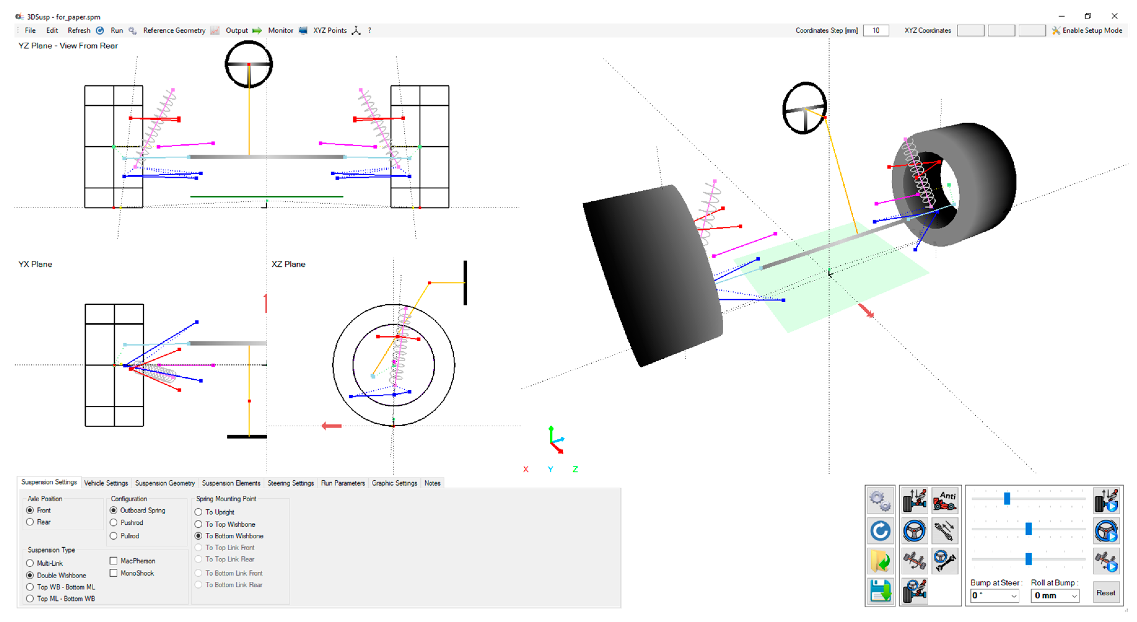
2.6. Suspension Kinematics and Its Effects

The correlation between steering geometry and the torque steer effects have been investigated by means of a self-developed software tool for suspension kinematic design and analysis (see Figure 8).

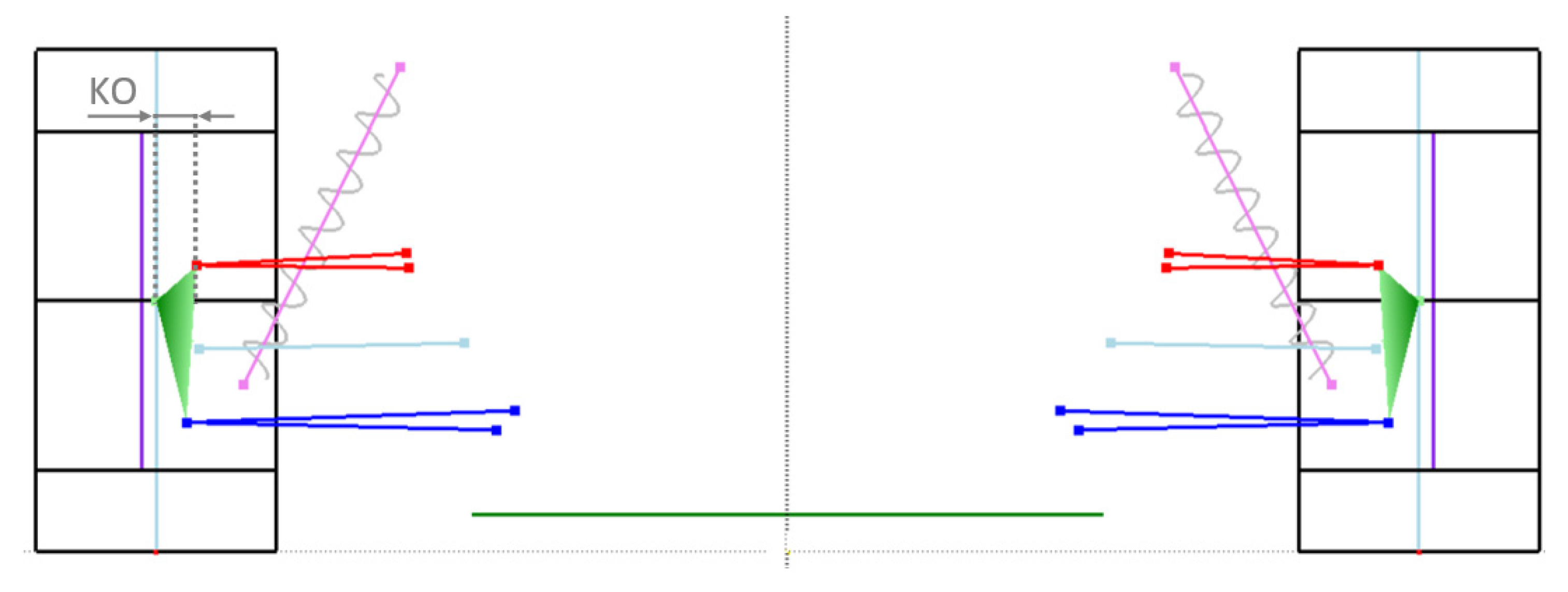
The reference geometry in Figure 9 is taken from the vehicle model. It appears suitable for a high-performance sportscar, as it is a little extreme, given the high value of the caster angle. Camber is kept to zero for simplicity. Additionally, the overall steering ratio (steering wheel angle/wheel angle, Sa/Wa) is fairly direct, hence it can be classified as “sporty” or “reactive”, see

Table 1. EB0 suspension compared with the original one.

Name	Caster [deg]	Kingpin [deg]	SR [mm]	CT [mm]	KO [mm]	Sa/Wa [deg/deg]
Original	10.2	14.2	16.1	29.0	102	15.7
EB0	5	3.7	29.2	12.5	51.4	15.5

.

The first modification, called EB0, was aimed at making the geometry more representative of a wider range of cars, and therefore with less aggressive caster and kingpin settings. This in turn allows for the kingpin offset (KO) to be halved (Figure 10 and Table 1). According to the formulas in chapter 2, all these three parameters have a large influence on torque steer, as shown later.

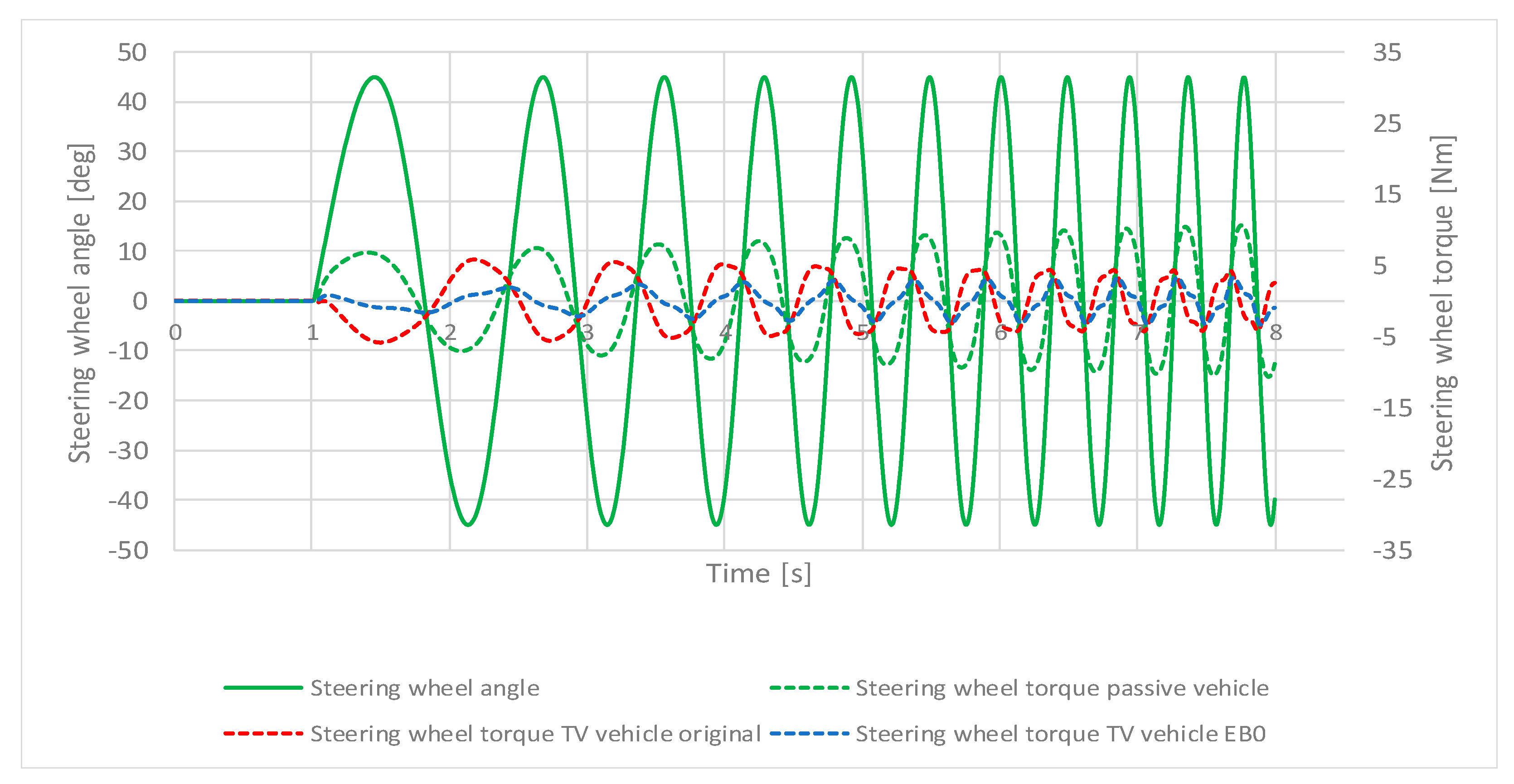
Figure 11 shows a comparison between the steering effort required for a sine steer sweep manoeuvre with the passive vehicle equipped with the original and EB0 front axle geometries, with the latter requiring reduced effort and driver involvement. However, the phase and shape are unaltered, thus giving an intuitive, “friendly” feedback in both cases because the steering effort remains on the self-aligning side.

2.7. Torque Vectoring and Its Effects

A description of the strategy adopted for typical torque vectoring (TV) control in itself is beyond the scope of this paper, and so is the related impact on vehicle balance, handling dynamics, and stability. Therefore, an over-simplified open-loop TV logic was purposely built within MATLAB-Simulink^® and simulated through co-simulation. The TV action in terms of torque difference, left to right, is proportional to the steering wheel angle and is directed at reducing understeer. That means the outer wheel torque is higher than the inner wheel torque, so the torque at wheel is:

C[Nm] = k[Nm/rad] ∙ SW_angle[rad]

(19)

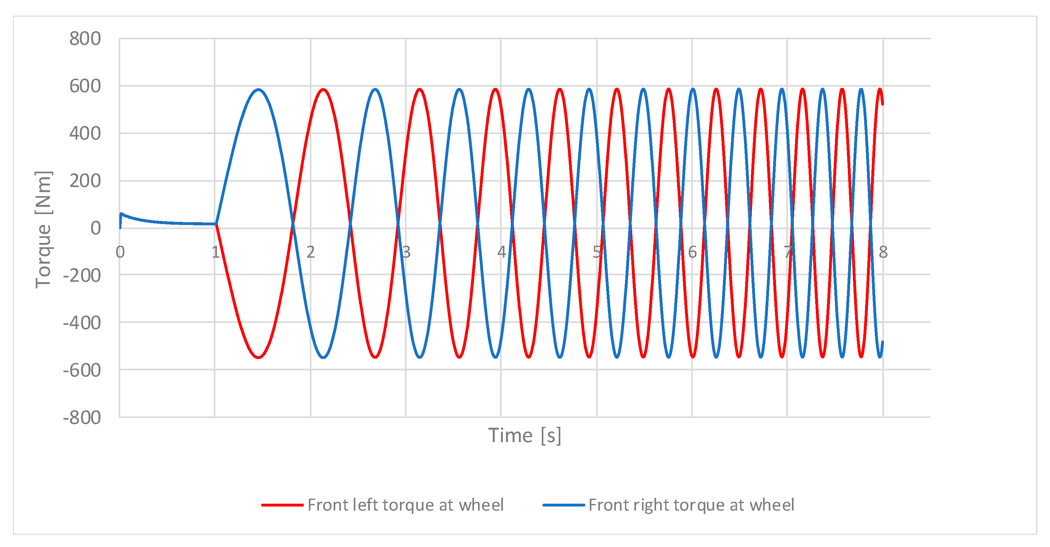
Figure 12, obtained by a sine sweep steer test, shows the torque delivered to the left-hand and right-hand side wheels being strongly differentiated to achieve a yaw moment by means of the torque vectoring action.

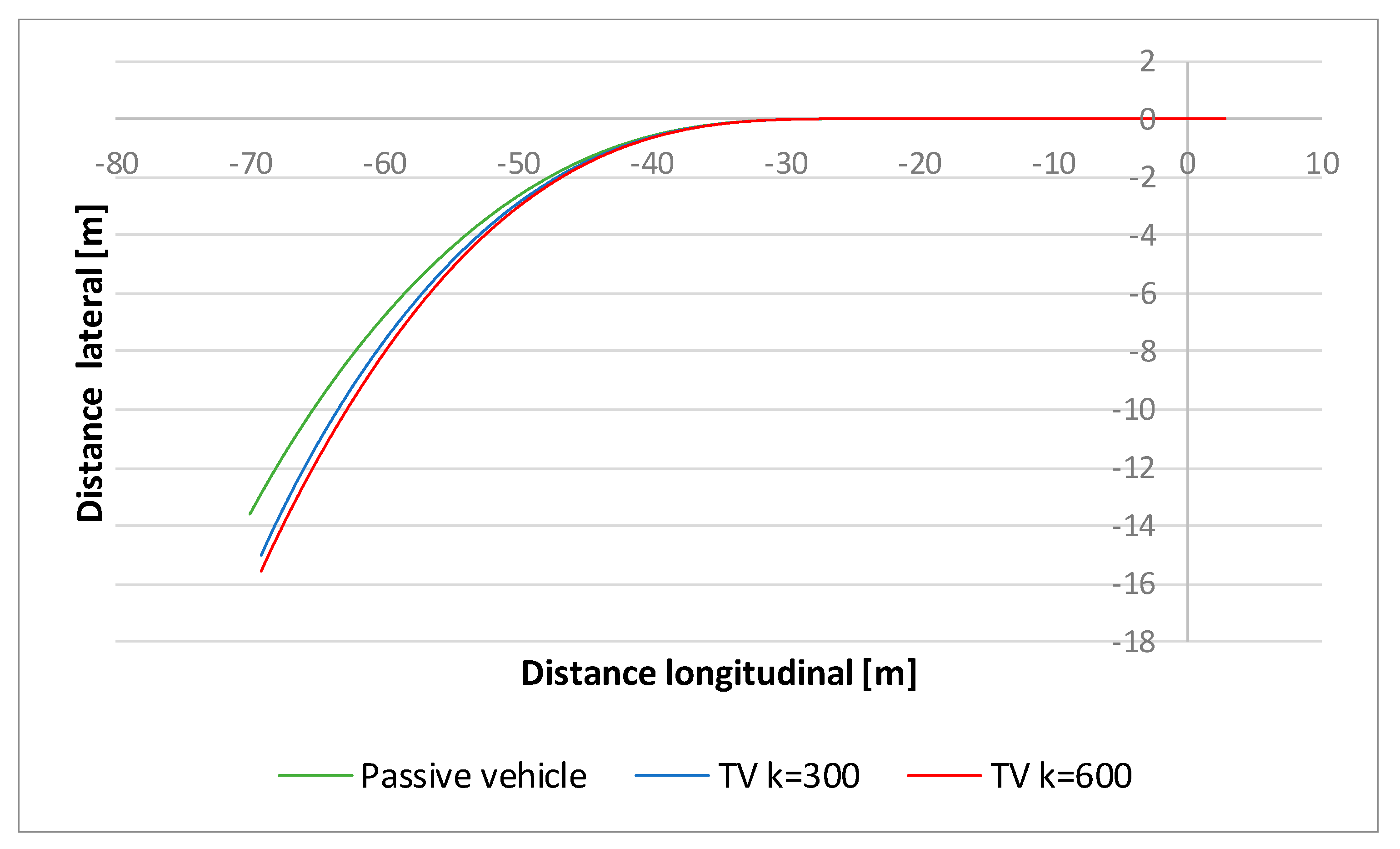
Two values of coefficient k (300 and 600 Nm/rad) were tested. The vehicle balance change in terms of the understeer reduction is shown in Figure 13 for a 90° step steer test at 80 km/h. A higher value of k results in less understeer and a smaller cornering radius as expected.

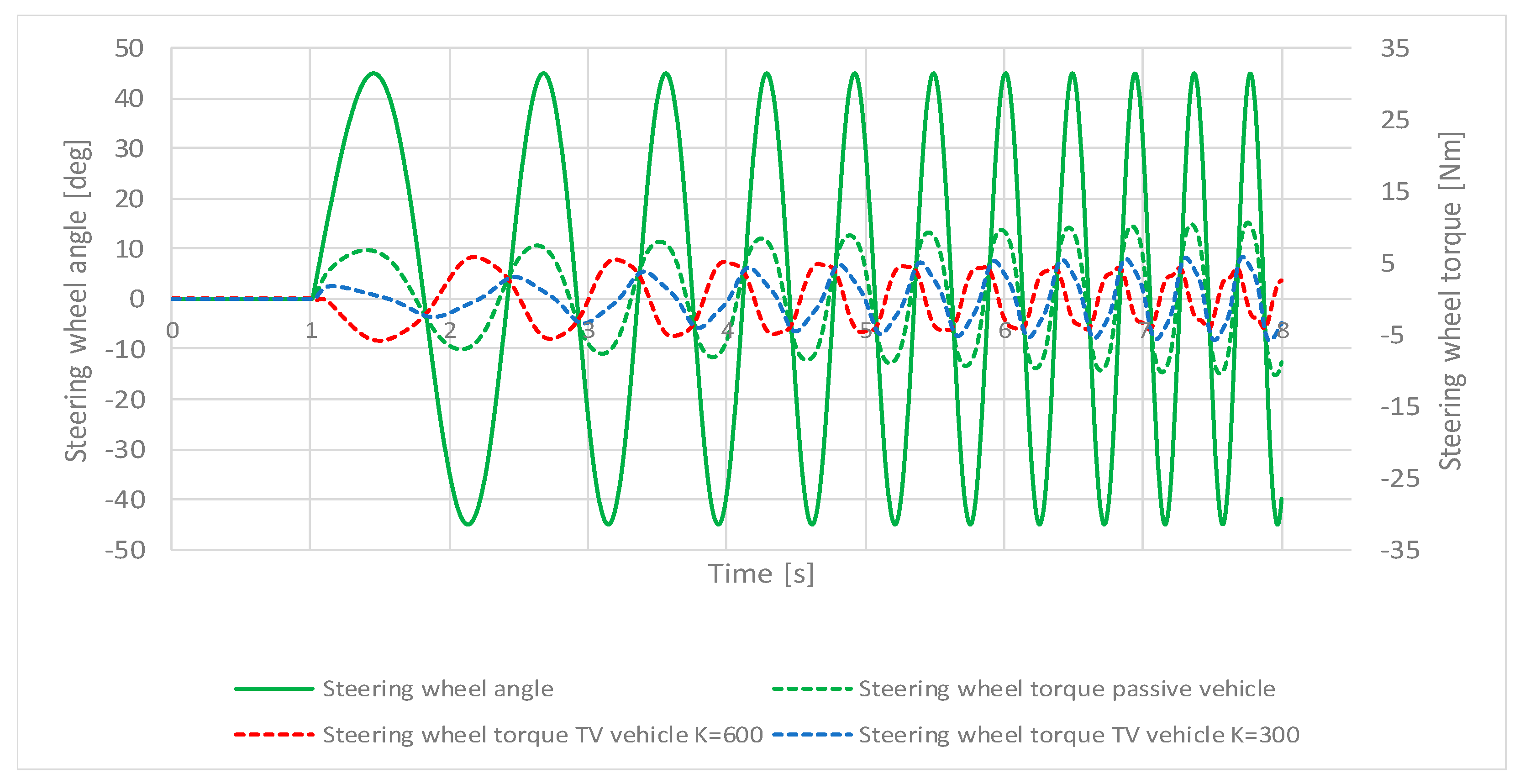
Figure 14 compares the steering wheel torque required with the passive vehicle (dotted green line) and with torque vectoring (k = 300 dotted blue line, k = 600 dotted red line), with the standard geometry in all cases.

It shows that the disequilibrium in terms of torques and longitudinal forces Fx at the ground affects the shape, linearity and phase of the steering effort required. The adverse effects are even more evident in the driver-in-the-loop simulator: the TV coefficient k = 600 Nm, in particular, results in a surprising and confusing feedback, and in the onset of steering instability, with the phase shift inducing an undesirable self-steering effect and jeopardising the driving feeling; the vehicle model becomes literally undriveable. From now on, all simulations will be performed with k = 600 because this appeared as the most critical case.

Figure 15 shows the steering effort required with torque vectoring applied to the EB0 modified geometry. The reaction is similar to the standard geometry with TV and k = 300, so the negative effects affecting steering feedback are somehow mitigated; the phase shift is reduced, but the response is still very far from the desirable curve obtained with the passive vehicle, as it can also be perceived in the driving simulator.

3. Results

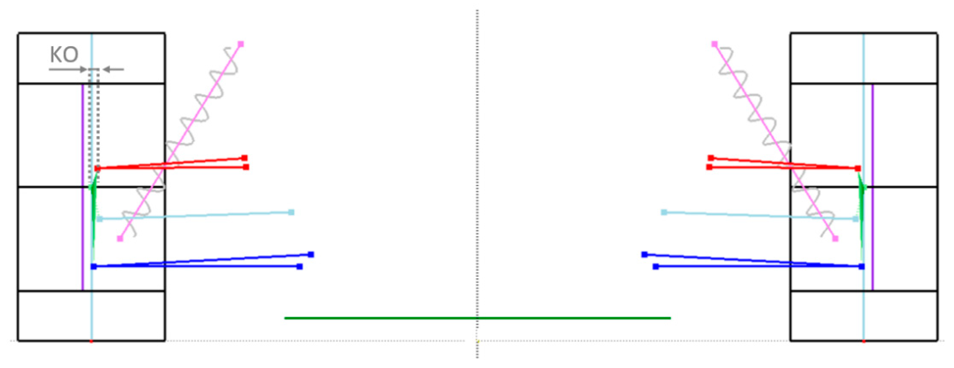
From here, different suspension geometries have been proposed with the aim of possibly restoring a stable and intuitive steering response regardless of the disequilibrium induced by the torque vectoring at the front, while maintaining at least the same overall steering ratio, and without claiming to achieve a definitive configuration. As a matter of fact, the refinement of the self-aligning properties given by the combination of tyre characteristics and steering geometry would certainly require more insight and fine tuning. Additionally, the compatibility with the design of the wheel group itself would require further evaluation, where the wheel group is composed by the wheel, the upright/brake assembly, the CV joint/driveshaft assembly, etc. The second variation (EB1) was designed to reduce the kingpin offset (KO) (Figure 16 and

Table 2. New EB1 suspension compared with the previous ones.

Name	Caster [deg]	Kingpin [deg]	SR [mm]	CT [mm]	KO [mm]	Sa/Wa [deg/deg]
Original	10.2	14.2	16.1	29.0	102	15.7
EB0	5	3.7	29.2	12.5	51.4	15.5
EB1	5.3	2.1	−1.2	30.2	11.4	15.0

).

After the same sine steer sweep test, the steering wheel torque of EB1 is shown in blue in Figure 17. Apart from a small phase shift at low frequency, the steering effort is very similar to the reference case.

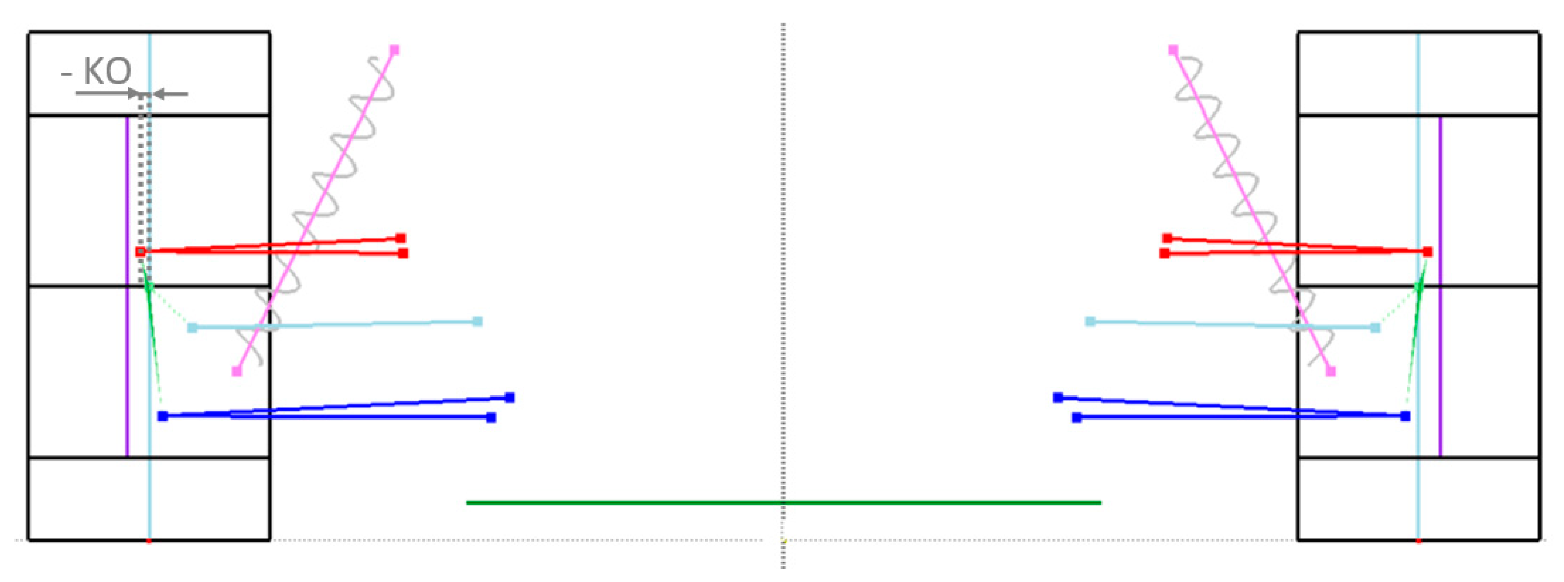
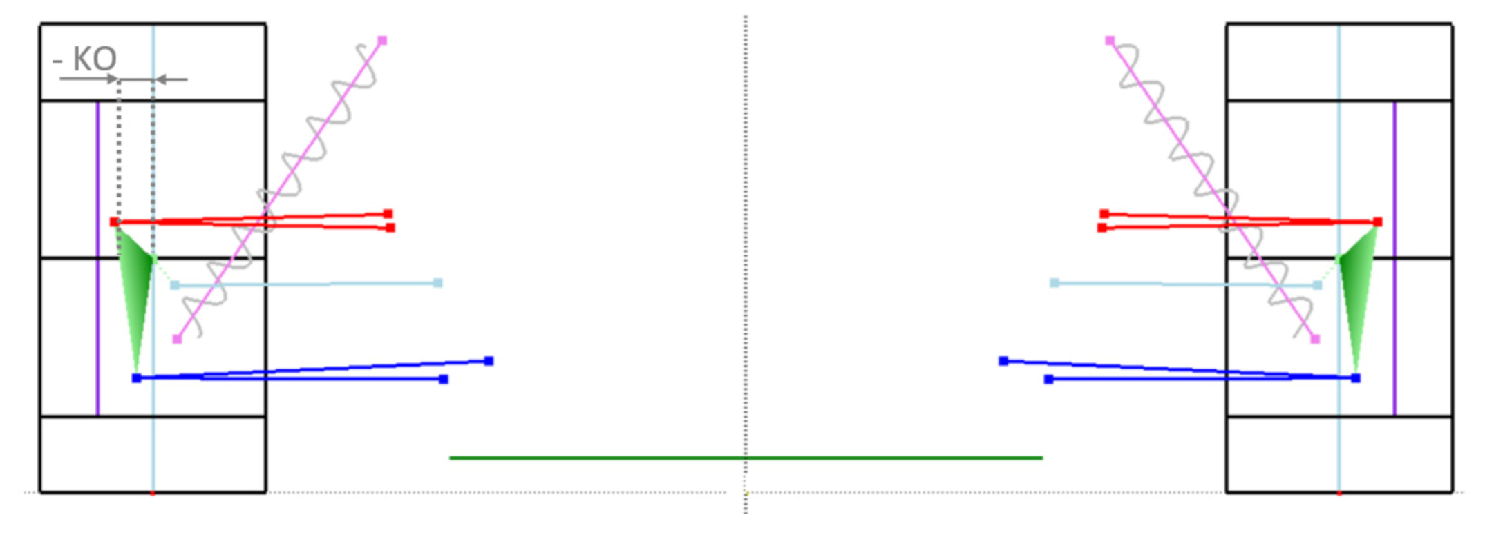
At this point, further variations were designed with a small, negative KO (−5.6 mm, EB2, Figure 18) and with a very large negative one (−48.9 mm, EB3, Figure 19 and

Table 3. New EB2 and EB3 suspensions compared with the previous ones.

Name	Caster [deg]	Kingpin [deg]	SR [mm]	CT [mm]	KO [mm]	Sa/Wa [deg/deg]
Original	10.2	14.2	16.1	29.0	102	15.7
EB0	5	3.7	29.2	12.5	51.4	15.5
EB1	5.3	2.1	−1.2	30.2	11.4	15.0
EB2	3.9	−7.8	40.8	16.4	−5.6	15.3
EB3	4.8	−8.1	−0.3	19.0	−48.5	15.0

).

EB3 in particular features a larger amplitude in terms of self-aligning torque, as shown in Figure 20. Again, although this is a self-aligning torque, in the simulator, the amplitude reveals itself to be too much of an effort, hence it is not desirable and calls for very small values of KO, which in turn is in agreement with vehicle dynamics experience and theory.

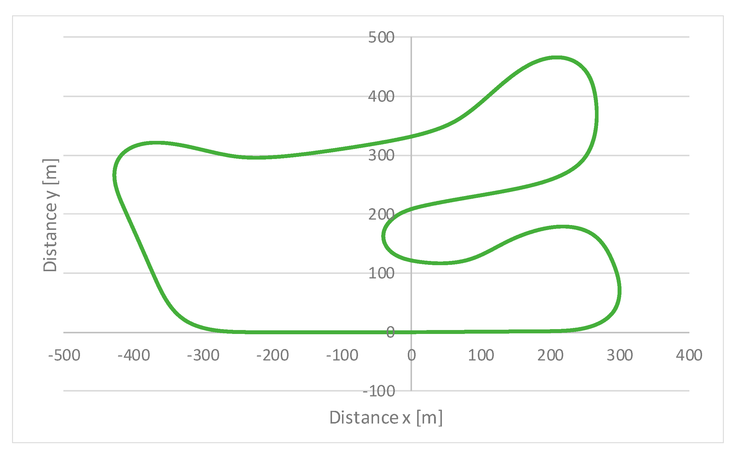
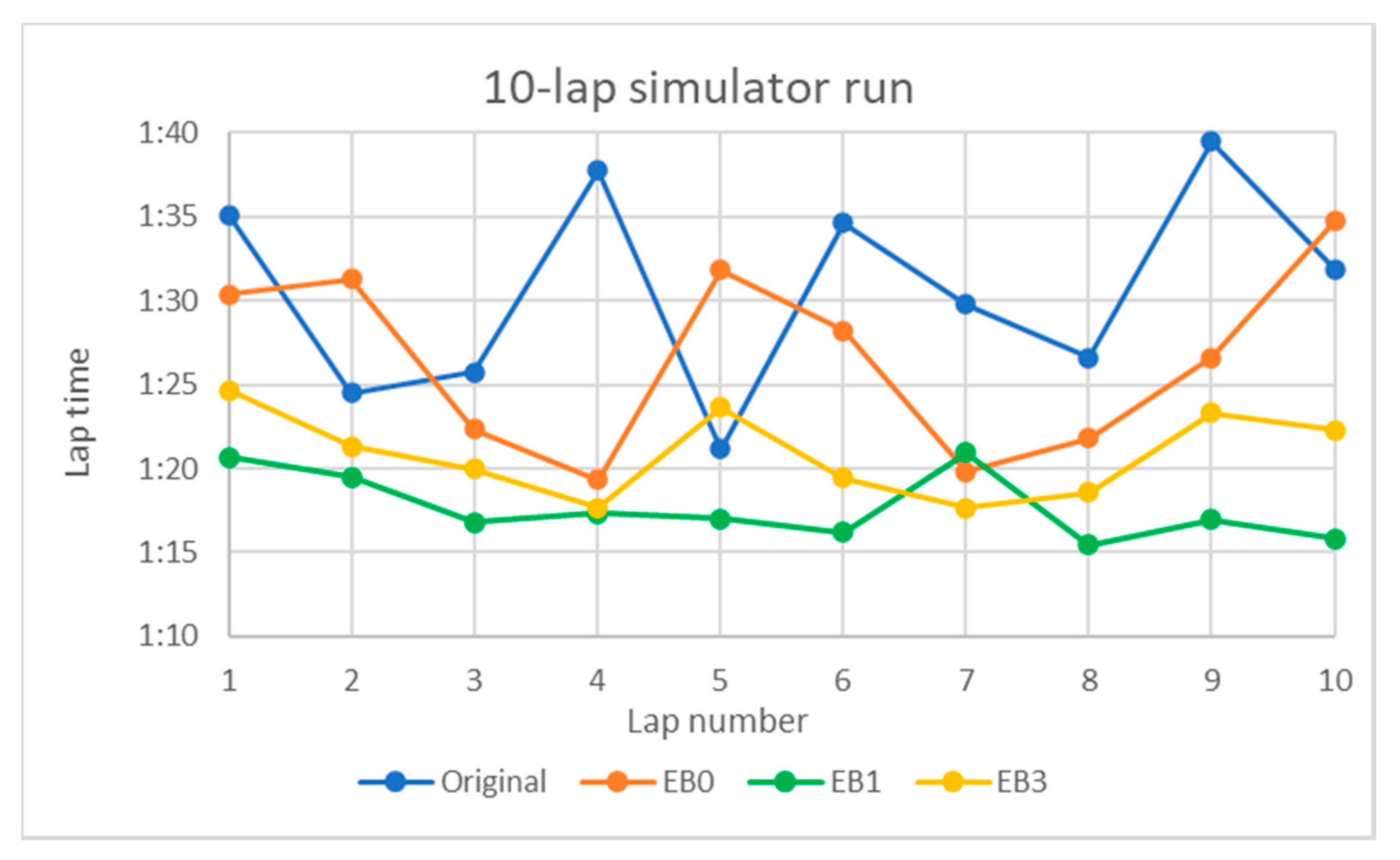
For the sake of completeness, in order to verify the global performance of the vehicle, additional offline simulations were carried out on a lap of the Hockenheim short track (Figure 21), a circuit featuring either slow and fast corners and quick changes of direction, often considered to be representative for handling evaluations. The original, passive vehicle (without torque vectoring) is compared with the application of TV to the various kinematic variants. Fast laps on the driving simulator were also performed by an experienced driver in order to assess the performance potential of each solution, the subjective feeling and also the consistency of consecutive lap times, the latter often being considered as a meaningful indicator of driving intuitiveness and stability, especially in motorsport.

The steering wheel angle and steering effort in the space domain along the circuit are shown in Figure 22, Figure 23, Figure 24, Figure 25 and Figure 26 for all configurations analysed in the previous chapter. The vehicle options are driven on a fixed trajectory by VI-grade’s Virtual Driver model, therefore, the subjective driver assessment on the vehicle balance and optimum racing line is removed from the equation.

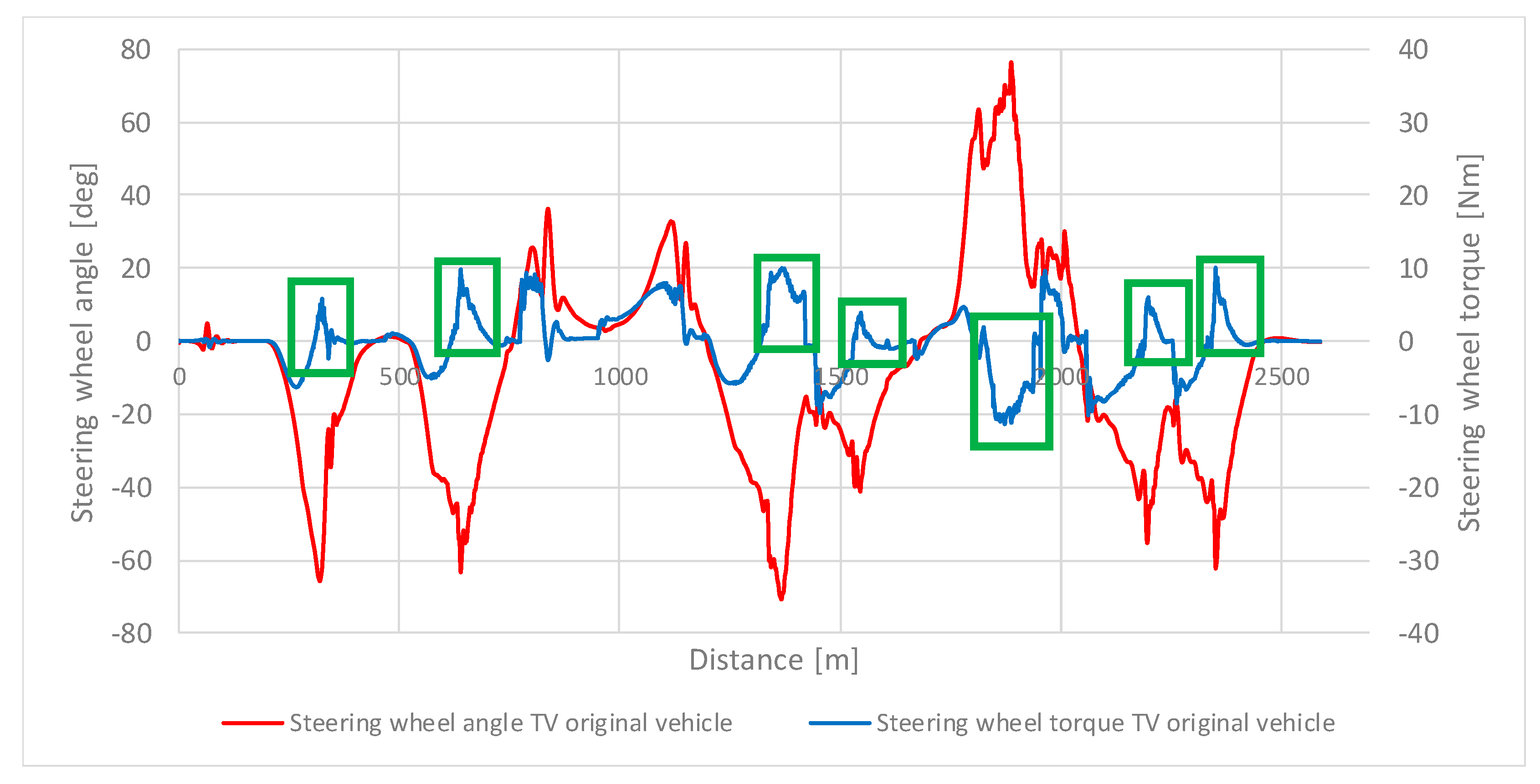
The passive vehicle behaviour with TV off and standard geometry is shown in Figure 22. Steering angle and steering wheel torque always have the same sign; this is the desirable situation of self-aligning torque feedback to be taken as a reference, which also makes driving on the simulator a natural and intuitive process, as shown by lap time consistency.

Like in the sine sweep test, torque vectoring on the original vehicle geometry causes a large self-steering moment in most of the corners (green boxes in Figure 23). This is where the torque and steering angle have opposite signs. Driving this configuration on the simulator immediately demonstrates how difficult it would be to drive a powerful car at racing pace (i.e., very close to the limit of adherence) without the re-assuring self-aligning steering torque a feedback: the driver has to “fight” the steering all the time. Consecutive lap times are slow and extremely inconsistent (Figure 27) because the vehicle behaviour and trajectory are scarcely predictable.

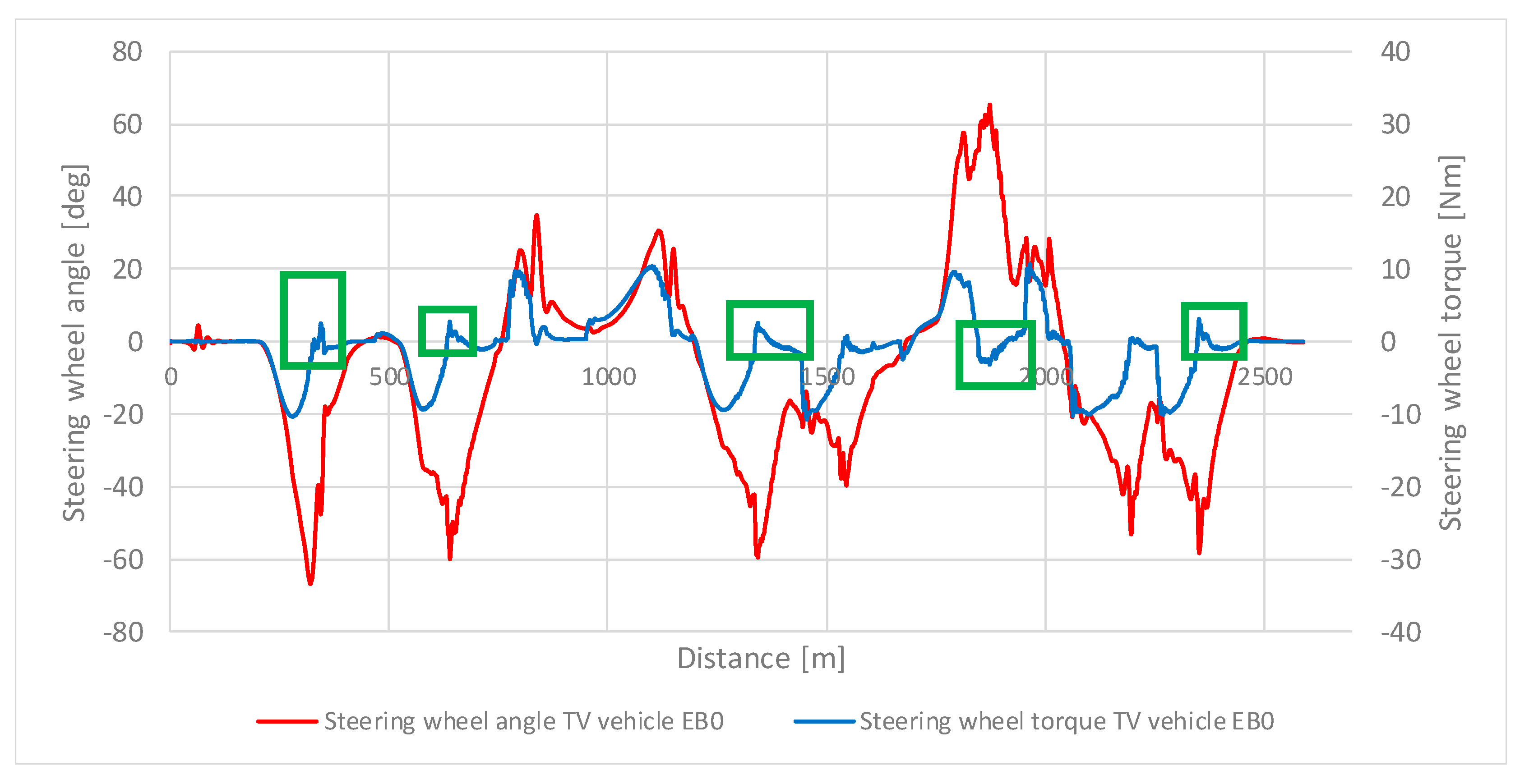
With the EB0 suspension, designed to reduce KO, although still matching wheel assembly components, the result is better but occasional self-steering peaks are still visible (Figure 24). In the simulator, this effect can be clearly detected after a few laps. Driving at the limit is still very stressful and the pace is inconsistent; the lap time improves after a typical learning cycle, then they tend to increase again, this is probably due to the driver’s mental fatigue.

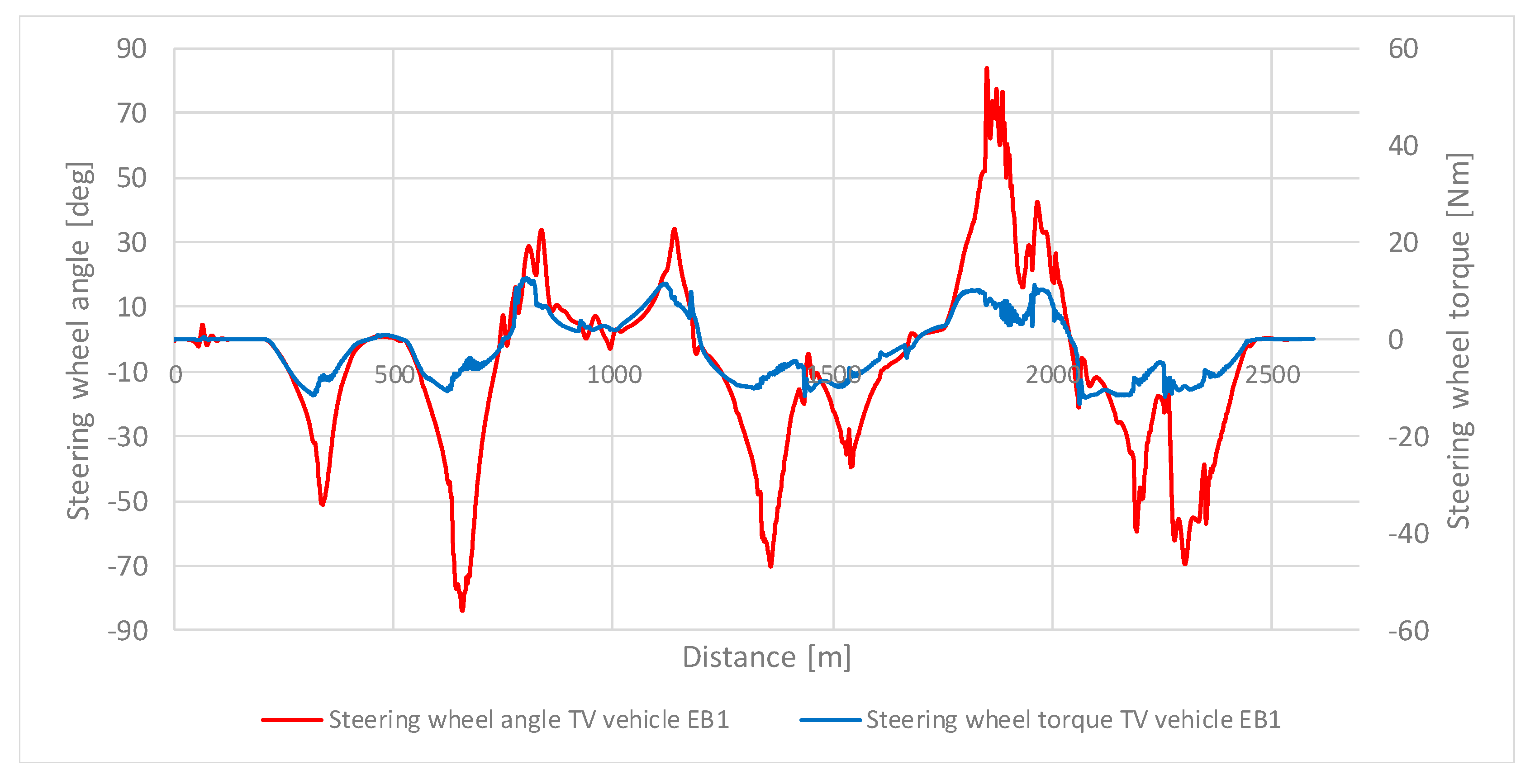
As in the previous section, the most balanced results, i.e., the closest to the reference passive case, have been obtained with the EB1 geometry (KO = 11.4 mm, Figure 25).

This basically deletes the interaction between the differentiated torque delivery due to TV and steering, thus making TV application possible. Self-steering effects are totally removed and the steering feel on the simulator is back to a reassuring, natural effort, helping the driver to establish the abovementioned intuitive correlation between cornering speed, steering angle and steering effort, and to perceive vehicle balance. Lap times are faster overall and consistent.

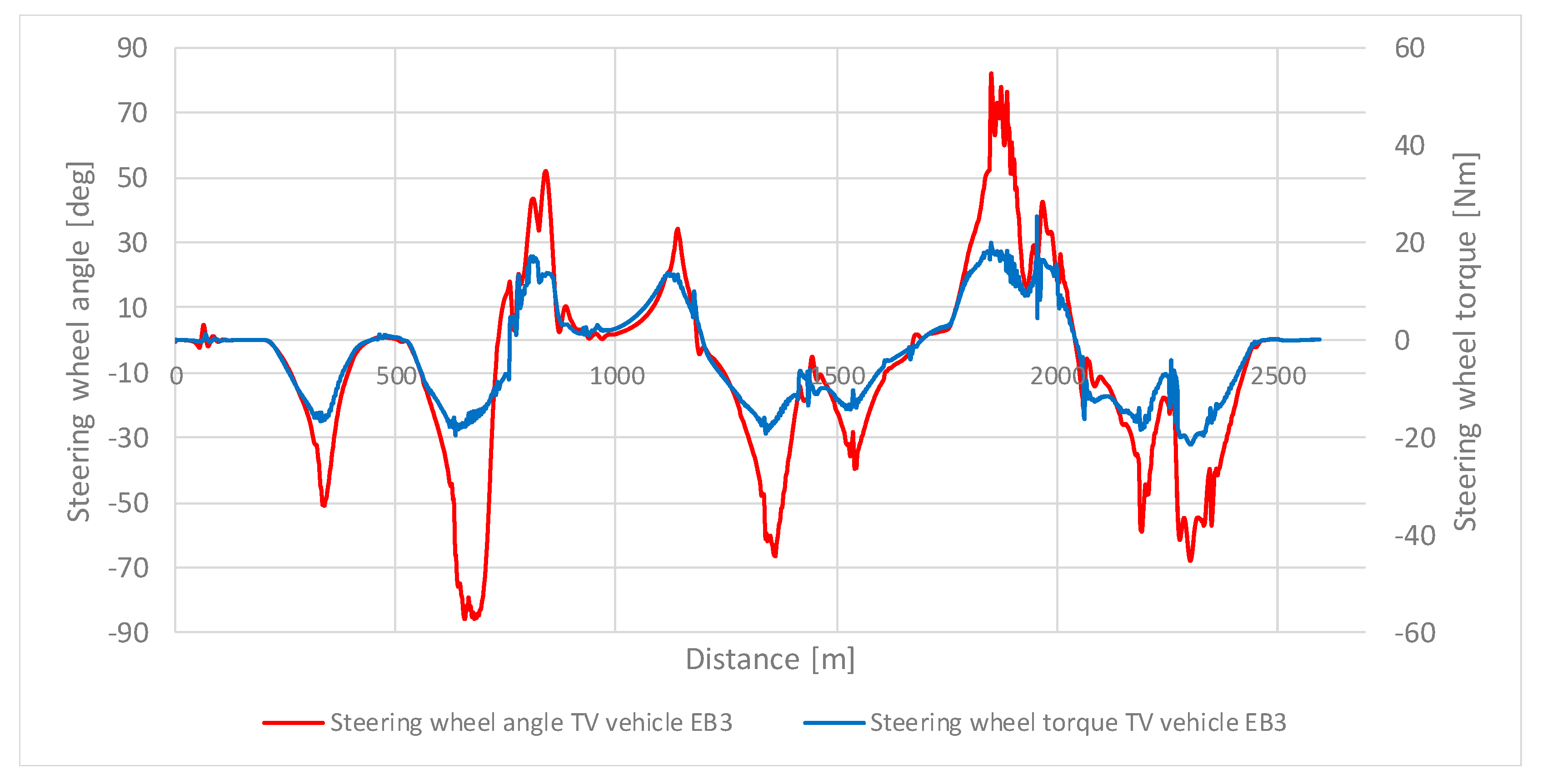
The EB3 geometry (KO = −48.5, Figure 26) basically amplifies the self-aligning effect, which is a good thing in itself. However, it also restores the undesirable interaction between torque delivery (under power for instance) and steering feel and driving on the simulator once again becomes less intuitive and more stressful, as shown by the fairly poor lap time consistency. The overall steering effort is also harder.

4. Conclusions

This paper aims at describing the application of torque vectoring on the vehicle front axle by means of two separate electric motors. TV can offer potential benefits in terms of handling and stability at the expense of steering feel, and ultimately performance, if torque steer effects are not taken into account during the design phase. The analysis of different suspension/steering geometries shows that the kingpin offset (KO) has a strong influence on torque steer. It should be minimised, provided the resultant geometry is compatible with the design of the wheel assembly.

Finally, it should be stated that the net force exchanged between the rolling tyre and the road is inevitably applied to a point wandering within the contact patch area, especially on uneven surfaces. Therefore, the effective KO amount is not a fixed distance and it is not possible to eradicate torque steer effects completely, especially with modern wide tyres.