Quality Monitoring for Micro Resistance Spot Welding with Class-Imbalanced Data Based on Anomaly Detection

Abstract

Micro resistance spot welding (MRSW) is an important technology widely used in electronics manufacturing for micro component joining. For the joining of micro enameled wire, quality control is heavily dependent on manual inspection till now. In this paper, a quality monitoring approach based on isolation forest (iForest) is proposed to identify abnormal welds and normal welds. Electrode voltage and welding current of over 110,000 spot welds were collected from a production line. The dynamic resistance and heat input were calculated for all welds and used for feature extraction. A class imbalance problem existed in the collected dataset because abnormal welds were far fewer than normal welds. The anomaly detection model based on iForest was established for the imbalanced data classification after comparison with other methods such as one-class (support vector machine) SVM and local outlier factor. Test results show that the similarity of dynamic resistance profile and heat input compared with the previous ten welds are valid features for detecting a part of the abnormal welds. The iForest model is effective for distinguishing incomplete fusion welds from normal welds with high efficiency. It can assist in the on-line quality monitoring of enameled wire welding process in production.

1. Introduction

With the booming development of miniaturization and integration of electronic devices, micro enameled wires have been increasingly used in the manufacture of various electronic products, such as electroacoustic devices, micro coils, micro delay and chip inductor et al. [1,2]. The micro resistance spot welding (MRSW) of enameled wire to pad is a common production process, since the removal of insulation coating and the joining of wire to pad can be accomplished efficiently in a welding process. Because of advantages such as low cost, high efficiency and ease of automation, MRSW is an important micro joining technology for the manufacture of micro devices, which is also termed small-scale resistance spot welding [3,4].

In view of the demand of reliable signal transmission in electronic components, especially the high fidelity requirement of electroacoustic devices in smartphones and earphones, it is important to ensure the quality of each MRSW weld. However, quality control still relies heavily on manual inspection, which requires experienced people to do it with great attention and still overlooks some defects. It is essential to realize on-line quality monitoring.

Several studies have recently focused on the quality control of MRSW [4,5,6,7,8]. Wan et al. [4] developed a weld quality evaluation model based on electrode voltage recognition for the MRSW of 0.4-mm-thick titanium alloy sheets. Wan et al. [5] compared the quality assessment performance between back propagation neural network (BPNN) and probabilistic neural network (PNN) in MRSW, and it was concluded that BPNN was more appropriate for failure load estimation and PNN was more effective at quality classification. Yue et al. [6] established regression equations between welding parameters and weld quality with response surface methodology for foil metal joining. Chen et al. [7] designed multi-performance optimization for MRSW with a hybrid approach. Rikka et al. [8] optimized the welding parameters by Taguchi design to obtain low electrical contact resistance for joining a nickel tab to an inner aluminum casing in a cylindrical cell. However, despite the great demand in industry, there is a lack of investigation into quality monitoring in the MRSW for micro enameled wire joining.

Quality assessment for resistance spot welding (RSW) has been studied extensively [9,10]. Different process signals are analyzed for feature extraction, such as dynamic resistance [11], welding power [12], electrode force [13], electrode displacement [14] and multiple signals [15]. Dynamic resistance has wide application because of the low cost and convenient installation of sensors. In recent years, machine learning models have been found to be effective for predicting weld quality, including artificial network [16,17], decision tree [18], random forest [19] and SVM [20]. The rapid development of machine learning technology provides effective decision support tools for weld quality evaluation.

Despite comprehensive studies on the weld quality of MRSW and RSW, specific applications require further investigation. First, compared with RSW or MRSW of metal sheets, MRSW of enameled wire to pad is quite a different physical process and has rarely been explored before. Additionally, a class imbalance problem exists in the quality classification of MRSW in the production. This refers to data within which one or more of the classes (majority class) have a much greater number of samples than the others (minority class) [21]. As a result of quality control, abnormal welds are generally far fewer than normal welds in the manufacture of micro components by MRSW. Traditional classification models cannot provide good performance for class-imbalanced data, which requires imbalanced data processing methods like anomaly detection algorithms [21].

Based on an imbalanced dataset from industry, this work focuses on the quality monitoring for MRSW of micro enameled wire to pad. The welding process was analyzed in terms of dynamic resistance and heat input, and they were adopted for feature extraction. A classification approach based on isolation forest (iForest) is proposed to assist in the quality inspection.

2. Materials and Methods

2.1. Materials and Equipment

Enameled copper wire with a diameter of 0.08 mm was joined to the 1.5 × 1.5 mm pad coated with 0.01 mm thick tin solder in an electronics factory. A direct current (DC) welder was used to heat the tungsten electrode, as shown schematically in Figure 1. The joule heat was generated intensively at the electrode tip and transferred to workpieces. The constant voltage control mode was selected for micro enameled wire joining, since it had better adaptability than constant current and constant power, which made the welding current vary in the welding process.

The welding parameters are listed in

Table 1. Welding parameters.

Number of Heating Pulse	Voltage Setting (V)	Welding Time (ms)	Electrode Force (N)
2	0.68–0.90	55–60	5.2

. All welds were produced by applying double heating pulses. The 1st pulse was used to remove the insulation coating from the wire, and the 2nd pulse was set up to provide enough heat. The voltage setting was varied in the range of 0.68–0.90 V, because it matched with each electrode and was adjusted manually during the electrode life. The welding time was varied from 55 to 60 ms due to its fine-tuning for each electrode.

2.2. Process Data Aacquisition

The instantaneous electrode voltage (u_t) and welding current (i_t) of 111,958 spot welds were collected by the data acquisition system shown schematically in Figure 1. The curves of u_t, i_t and dynamic resistance (R_t) were saved for each weld. A weld performed in the early and middle stage of electrode life is taken as an example in Figure 2. Part of the resistance curve is ignored because u_t and i_t change rapidly between the two pulses, making the curve change abruptly.

2.3. Weld Quality Determination

The quality of each weld was estimated by manual visual testing. The quality level was divided into two classes: ‘normal’ and ‘abnormal’. As listed in

Table 2. Visual testing results.

Normal Welds	Incomplete Fusion	Abnormal Wire	Overheating	Other Failures	Defectrate
111,905	21	22	8	2	<0.25%

, 53 abnormal welds were recorded in detail in the MRSW dataset, including four defect types: incomplete fusion, abnormal wire, overheating, and other failures.

It is a class-imbalanced dataset, since abnormal welds (the minority class) are far fewer than normal welds (the majority class). Classifying imbalanced data significantly challenges traditional classification models: (1) their bias towards the majority class causes poor identification for the minority class, (2) minority samples usually overlap with majority samples in part of the characteristic space, which is termed class overlap, and (3) there are very few minority samples or even there are only normal samples in specific applications [21,22]. It is more appropriate to select anomaly detection algorithms rather than traditional classification methods for quality classification of imbalanced data.

Despite the low defect rate (<0.25%), it is crucial to detect abnormal welds because it is necessary to ensure the quality of each product. They cannot be avoided completely due to various disturbances at production sites. Moreover, it is virtually impossible to make a redundant welding spot on the pad to reduce the failure risk, which makes quality monitoring critical.

2.4. Welding Process Analysis

For joining micro enameled wire to tinned pad by MRSW, the basic principle is that the joule heat is generated at the electrode tip by passing an electrical current to remove the insulation coating from the wire and re-flow the solder on the pad. The wire is joined to the pad under a controlled pressure. The weld energy required is obtained from the heated electrode by heat transfer. It is different from the sheet metal joining by RSW or MRSW, where the heat is generated at the interface of the sheets.

Figure 3 shows four signal curves of MRSW from the perspective of electrode life. One of the electrodes is shown as an example: voltage control setting (V_CON), average of I_t in a welding process (I_AVE), initial resistance (R₀, the first resistance value collected in a welding process, shown in Figure 2) and heat input of electrode and workpieces (Q_E). For I_AVE, R₀ and Q_E, the moving averages of every 200 welds are calculated to make the trends clear. As welding number grows, Figure 3 shows that V_CON is reduced manually (from 0.86 to 0.76 V), I_AVE and Q_E decline in general (from 177 to 88 A, from 8.2 to 3.6 J), while the R₀ curve shows an upward trend (from 2.5 to 8.3 mΩ).

2.4.1. Dynamic Resistance

For the sheet metal joining by RSW in industry, the measured voltage is composed of a resistive and an inductive component: u_RSW = iR + Ldi/dt [23,24]. The induced voltage is picked up by the two electrical wires which span the upper and lower electrodes and form an inductance loop [24]. However, for the micro enameled wire joining by MRSW with single electrode, there is not an obvious inductance loop for the u_t measurement (Figure 1c). The R_t is obtained through dividing u_t by i_t in this study.

As shown in Figure 4, the equivalent circuit for the electrode and workpieces can be regarded as resistance in series-parallel connection. R_E represents the resistance from the voltage measuring position to the electrode tip, R_Tip represents the electrode tip resistance, and R_W is used to analyze the workpiece resistance and the contact resistance. The following factors influence R_t and its profile.

• Factor 1: the electrode wear. This is caused by several factors, such as frequent tip cleaning and ignition loss, which causes the mass and the size of the tip to decrease (Figure 4b) and R_Tip to increase as the welding number grows [2].
• Factor 2: the temperature increase. The electrode temperature increases because of the net energy input of electrode, and the heat transferred to the workpieces also causes their temperature to increase. Therefore, the resistivity of the electrode and workpieces increases in the welding process.
• Factor 3: the shunting effect. Because of the low resistivity of copper, more or less of the current is diverted to the joint of copper wire to the pad. The R_W starts to influence R_t after the insulation coating is removed. When the R_Tip becomes higher in the middle and late stage of the electrode life, the resistance curve may drop obviously due to the shunting effect.

According to the change of R_t profile during the electrode life, it is divided into several types based on its main trend described in

Table 3. Notation of dynamic resistance profile.

Main Trend	Pulse	Code	Notation
Up	1st	0	Rt keeps rising mainly.
Up&Down	1st	1	Rt starts to rise and then a drop occurs. However, it does not decline in general.
Down	1st	2	Rt declines in general since its decline is obviously greater than its rise.
Up	2nd	0	Rt keeps rising mainly.
Flat	2nd	1	Rt has obvious stages of slight change despite the local increase.
Down	2nd	2	Rt declines in general despite the local increase.

. One of the electrodes is taken as an example in Figure 5 to show the change of R_t. Figure 6 shows various profiles with arrows used to point out the main trends. Its change can be explained by the above factors.

• Factor 1: its effect can be observed from the R₀, due to the slight effect of Factor 2 and Factor 3 when the welding just starts. After the electrode has been used for a long time, it is prone to wear out, which is reflected in the steep rise of R₀. It can be observed in Figure 3 also.
• Factor 2: it generates the ‘Up’ profile, which is the majority of the resistance curves shown in Figure 5.
• Factor 3: it can be seen obviously in the middle and late stage of electrode life. After the removal of the insulation coating, part of current is shunted to the wire and the pad, causing R_t to drop to some extent. Figure 5 shows the ‘Up&Down’ profile, but the ‘Down’ profile may occur because of the greater effect of Factor 3 than that of Factor 2.
• The balance between Factor 2 and Factor 3 may result in the ‘Flat’ profile.

The profile code listed in Table 3 was attributed to each resistance curve by the trend determination rules written in Python. As listed in

Table 4. Ratios of different profile types (%).

Profile Type	Ratio	Profile Type	Ratio	Profile Type	Ratio
Up–Up	59.68	Up&Down–Up	26.86	Down–Up	2.10
Up–Flat	1.95	Up&Down–Flat	5.88	Down–Flat	0.65
Up–Down	1.73	Up&Down–Down	1.07	Down–Down	0.08

, ‘Up–Up’ and ‘Up&Down–Up’ have a majority of R_t profiles, accounting for 86.54% of the total weld count.

2.4.2. Heat Input

The Q_E is obtained based on the electric work formula $Q_E={\int }^{}{u}_t{i}_{t}dt$. As shown in Figure 3, the characteristics of Q_E during the electrode life include three aspects. (1) When the V_CON remains unchanged, Q_E decreases gradually as the welding number grows due to electrode wear. (2) The electrode is finally scrapped because of insufficient Q_E. (3) The V_CON is turned down manually during the electrode life. This is related to the following factors: the mass loss of the electrode tip, the heat generated at the tip and the heat transferred to the workpieces. The formula for specific heat capacity (Q = mcΔT) can be used for explanation. As welding number grows, the net energy input of the electrode decreases from Q₁ to Q₂ and its mass decreases from m₁ to m₂. However, if Q₂/Q₁ is greater than m₂/m₁, ΔT₂ will be greater than ΔT₁, which causes excessive heat transferred to workpieces. Actually, overheating will occur if the V_CON is not duly adjusted in this application.

2.5. Methods

2.5.1. Anomaly Detection Algorithms

For imbalanced data classification, the pattern of normal samples can be recognized by anomaly detection algorithms when the training set has only normal samples or it contains abnormal samples. The samples that do not fit the pattern are classified as anomalies. This is the basic principle of anomaly detection, which belongs to unsupervised learning. Three well-known anomaly detection algorithms are discussed for quality monitoring: Isolation Forest (iForest), One-Class SVM (OCSVM) and Local Outlier Factor (LOF).

The iForest ‘isolates’ a sample from the rest of samples by adopting an ensemble of random trees as base estimators for the decision. The number of separations required to isolate a sample is the normality measure of iForest, as it produces noticeably smaller separation numbers for anomalies [25]. OCSVM has good performance for capturing the shape of the training set which contains normal samples only [26]. Samples outside the shape frontier are regarded as anomalies. LOF is a well-known density-based method which identifies the samples with much smaller local density as anomalies [27].

2.5.2. Feature Extraction

Similarity is a common measure for distinguishing abnormal samples from normal samples. In terms of R_t profile and Q_E, most welds are similar to their ‘near neighbors’ (e.g., the previous 10 welds), because the R_t and Q_E in general change gradually during the electrode life. Compared with the ‘far neighbors’ (e.g., the previous 1000th–1010th welds), a large disparity may be observed due to electrode wear, especially for welds performed in the middle and late stage of the electrode life.

To quantify the profile similarity between the resistance curves of two welds (X and Y), a curve similarity measure S_p(X, Y) is constructed using Equations (1)–(3) to obtain the dimensionless feature in the range of [0.0, 1.0] [28]. This is based on Euclidean distance, which is widely used to calculate curve similarity [29]. For different cases (profile codes are equal or not), it has different parameter values to calculate the similarity score [30]. When the spot welds have the same profile code in the 1st or 2nd pulse (p = 1 or 2), S_p(X, Y) is in the range of [0.0, 0.5]. If not, S_p(X, Y) is in the range of (0.5, 1.0]. S_p(X, Y) is smaller when X and Y have more similar profiles.

$$E_p(X,Y)=\sqrt{{\displaystyle \sum _{i=1}^m{\left(x_i-y_i\right)}^2}}$$

(1)

$$D_p\left(X,Y\right)=\max \left(\frac{1}{m}{\displaystyle \sum _{i=1}^m{x}_i},\frac{1}{m}{\displaystyle \sum _{i=1}^m{y}_i},E_p(X,Y)\right)$$

(2)

$$S_p\left(X,Y\right)=\frac{1}{2}\left(A+\frac{E_p\left(X,Y\right)}{D_p\left(X,Y\right)}\right),A=\{\begin{array}{cc}0& ,C_p(X)=C_p(Y)\\ 1& ,C_p(X)\ne C_p(Y)\end{array}$$

(3)

where p represents the heating pulse (p = 1, 2), m is the number of R_t collected during the pulse, E_p(X, Y) is the Euclidean distance of X and Y in the 1st or 2nd pulse, D_p(X, Y) is the maximum of E_p(X, Y) and the averages of X and Y, C_p represents the profile code, and S_p(X, Y) is used to evaluate the profile similarity.

Two features calculated by Equations (4)–(7) are extracted from Q_E and R_t for anomaly detection: the similarity of Q_E (ΔQ₁₀) and the similarity of R_t profile (ΔS₁₀). Both of them are compared with previous 10 welds. There is no evident linear correlation between them because the absolute value of Pearson correlation coefficient is less than 0.12.

$$\mathsf{\Delta }{Q}_{10}=\frac{Q_{anlz}-Q_{ave}}{Q_{ave}},Q_{ave}=\frac{1}{10}{\displaystyle \sum _{i=1}^{10}{Q}_i}$$

(4)

$$\mathsf{\Delta }{S}_{1–10}=\frac{1}{10}{\displaystyle \sum _{i=1}^{10}{S}_1\left(X_{anlz},X_i\right)}$$

(5)

$$\mathsf{\Delta }{S}_{2–10}=\frac{1}{10}{\displaystyle \sum _{i=1}^{10}{S}_2\left(X_{anlz},X_i\right)}$$

(6)

$$\mathsf{\Delta }{S}_{10}=\sqrt{0.5\times \left(\mathsf{\Delta }{S}_{1–10}^2+\mathsf{\Delta }{S}_{2–10}^2\right)}$$

(7)

where symbol anlz represents the weld to be analyzed, i is the index of its previous welds, ΔQ₁₀ is the relative change of Q_E, and ΔS₁₀ is used to analyze the similarity of R_t profile in the double-pulse welding process. For the first two welds of each electrode, the ΔQ₁₀ and ΔS₁₀ are regarded as 0.0; for the 3rd to 10th welds, the nominal ΔQ₁₀ and ΔS₁₀ are compared with the previous two welds.

2.5.3. Model Construction

To conduct the anomaly detection experiments, the models are constructed with the training set including normal welds only. All the abnormal welds and the remaining normal welds are used for model verification, as shown in Figure 7. Each weld in the test set is classified as ‘normal’ or ‘abnormal’. The Python packages from scikit-learn [31] are used, and the major parameters are listed in

Table 5. Anomaly detection algorithms and their major parameters.

Algorithm	Major Parameters
iForest	trees = 100, subsampling size = 256, contamination (c) ∈ [0.01, 0.02, …, 0.49, 0.49999]
OCSVM	kernel = ‘rbf’, gamma = ‘scale’, nu ∈ [0.01, 0.02, …, 0.49, 0.49999]
LOF	neighbors = 20, contamination (c) ∈ [0.01, 0.02, …, 0.49, 0.49999]

.

Four performance measures are applied in this study: recall (also termed sensitivity), specificity, processing time, and the area under the receiver operating characteristic curve (AUC) [20]. Recall and specificity are calculated by Equations (8)–(9). True positive (TP), false positive (FP), true negative (TN) and false negative (FN) are four types of predicted results in binary classification. In general, minority class (abnormal weld) is regarded as positive case and majority class (normal weld) is termed as negative case. AUC is widely used to analyze the performance of a binary classifier. It is in the range [0, 1], and a good classifier has an AUC score near 1.

$$\mathrm{Recall}=\frac{TP}{TP+FN}$$

(8)

$$\mathrm{Specificity}=\frac{TN}{TN+FP}$$

(9)

As common for preprocessing in machine learning, the features ΔQ₁₀ and ΔS₁₀ are scaled into the interval of [0, 1] by normalization. The normalized value ΔQ_10N is calculated by Equation (10), and ΔS_10N is equal to ΔS₁₀, where Lim_L is the lower limit and Lim_U is the upper limit used for ΔQ_10N. Compared with the previous 10 welds, the welds with small changes in Q_E have ΔQ_10N near 0.5, and ΔS_10N near 0 reflects small change in the R_t profile.

$$\mathsf{\Delta }{Q}_{10\mathrm{N}}=\{\begin{array}{ll}0\hfill & ,\mathsf{\Delta }{Q}_{10}\le {\mathrm{Lim}}_{\mathrm{L}}\hfill \\ \frac{\mathsf{\Delta }{Q}_{10}-{\mathrm{Lim}}_{\mathrm{L}}}{{\mathrm{Lim}}_{\mathrm{U}}-{\mathrm{Lim}}_{\mathrm{L}}}\hfill & ,\mathsf{\Delta }{Q}_{10}\in ({\mathrm{Lim}}_{\mathrm{L}},{\mathrm{Lim}}_{\mathrm{U}})\hfill \\ 1\hfill & ,\mathsf{\Delta }{Q}_{10}\ge {\mathrm{Lim}}_{\mathrm{U}}\hfill \end{array}$$

(10)

3. Results and Discussion

The particularity of the quality classification in this study can be illustrated by the feature distribution of normal welds and abnormal welds shown in Figure 8. The Lim_L and Lim_U of ΔQ₁₀ are selected to –0.1 and 0.1, respectively, because 97.5% welds are at this interval. According to the statistical analysis, 52,291 welds meet the conditions of ΔQ_10N ∈[0.4, 0.6) and ΔS_10N ∈[0.0, 0.2), and 79.6% (89, 094) welds meet the conditions of ΔQ_10N ∈[0.3, 0.7) and ΔS_10N ∈[0.0, 0.5). This reflects the fact that most welds are similar to their ‘near neighbors’ in terms of Q_E and R_t profile.

It can be observed that in this imbalanced dataset, abnormal welds overlap with normal welds in part of the two-dimensional characteristic space. The combination of class imbalance and class overlap makes it difficult to construct the frontier of each class, which adds complexity for quality classification. The dataset of normal welds may contain certain abnormal welds because of misjudgment, which may make abnormal welds overlap ‘normal’ (misjudged) welds. However, the amount of such polluted data was limited, since the weld quality was inspected by two inspectors in this experiment.

The weld failure detection methods based on traditional classification models appear to be unsuitable to detect abnormal welds from the imbalanced data. First, such models generally adopt global performance measures such as prediction accuracy in the learning process. If all welds are predicted as normal welds, a high accuracy score (>99.75%) can be obtained because of the low defect rate (<0.25%), leading to poor detection of weld failure in this application. Second, traditional classification models are based on supervised learning for the class-balanced data in general, while there is not enough real data of weld failure available for model training and testing in this study, since the abnormal welds do not often occur in reality. Third, the problem of class overlap also makes it difficult to distinguish between normal welds and abnormal welds by traditional classification models.

It is an essential task to find out abnormal welds in the quality monitoring of MRSW. Figure 9 shows the performance difference of anomaly detection for three models and four defect types. The parameter c or nu provided in the packages is used to adjust the model decision function.

For the detection of incomplete fusion welds, both iForest and OCSVM can distinguish all the incomplete fusion welds from normal welds, at the cost of the decrease in the specificity. The LOF model appears to be unsuitable for this application because its recall of incomplete fusion welds cannot reach 100% when c is near its upper limit 0.5. For the detection of other defect types, none of these models can identify the abnormal welds effectively, since no valid features have been extracted from u_t, i_t and variables calculated from them so far.

To analyze the classification of incomplete fusion welds and normal welds further, AUC, specificity and processing time are adopted, as listed in

Table 6. AUC, recall and processing time.

Algorithm	AUC	Recall		Processing Time (s)
		Specificity of 90%	Specificity of 80%	Train	Test
iForest	0.9525	0.8633	0.9524	1.79	1.11
OCSVM	0.9047	0.6437	0.9037	53.29	9.46
LOF	NA	0.1429	0.2857	0.43	0.25

. The average training time and average test time over the range of c or nu are used to compare the model efficiency. The LOF model is time-saving for model construction in this application, but it cannot identify all the incomplete fusion welds. Hence, its AUC is regarded as NA. The performance of OCSVM for anomaly detection is not poor; however, it is relatively time-consuming to train and test the model. The identification of incomplete fusion welds and normal welds can be performed effectively and efficiently by the iForest model. It has a high AUC score of 0.9525, and it takes 1.79 s to train the model with over 60,000 welds in the training set, and 1.11 s to test over 47,000 welds.

In addition to identifying abnormal welds, the interpretation of anomalies is also important for quality monitoring. For incomplete fusion welds, one of them and its previous 10 welds are shown as an example in Figure 10a,c,d. It can be observed that this abnormal weld has a different R_t profile and smaller Q_E. The previous welds have an ‘Up&Down’ profile in the 1st pulse, while the abnormal weld has an ‘Up–Down’ profile in the double pulses. This implies that the insulation coating was not properly removed as designed in the 1st pulse for this abnormal weld. Since the welding time was fixed, this weld lacked enough energy to join the wire to the pad after the insulation coating was removed. Based on the assumption that normal welds are ‘many and similar’ and anomalies are ‘few and different’, the iForest model can detect incomplete fusion welds with good performance in this application.

For other defect types, one from abnormal wire welds is analyzed as an example (Figure 10b). It was caused by the deviation of wire position. As shown in Figure 10e,f, it overlaps with its previous 10 welds in terms of R_t profile. This is related to the characteristics of the MRSW process for micro enameled wire joining, implying that the case of abnormal wire which occurs in the early and middle stage of electrode life does not obviously influence the temperature rise of electrode tip and tinned pad. Therefore, there is no remarkable difference in either ΔQ_10N or ΔS_10N between normal welds and these abnormal welds, meaning that the models cannot detect them effectively.

Although only incomplete fusion can be detected by the present iForest model with good performance, it is favorable for the quality monitoring research for MRSW. Its detection requires inspectors to be experienced and focused, which makes it relatively difficult to perform visual testing in the production line, while the deviation of wire position can be identified as abnormal wire with relative ease by a machine vision system. To further separate various abnormal welds from normal welds, more features from other process signals are required to fully represent the welding process. Similar to RSW, the quality monitoring based on multiple signals may be better for MRSW than that based on electrical signals only. Electrode displacement, dynamic force and images before and after welding are expected to be added in future work to improve quality monitoring.

4. Conclusions

An anomaly detection model based on iForest is proposed to assist in the quality monitoring of MRSW. The work is based on a dataset with the class imbalance problem. In terms of the dynamic resistance and heat input, the change during the electrode life is analyzed, and features are extracted from them for anomaly detection. The following conclusions can be obtained.

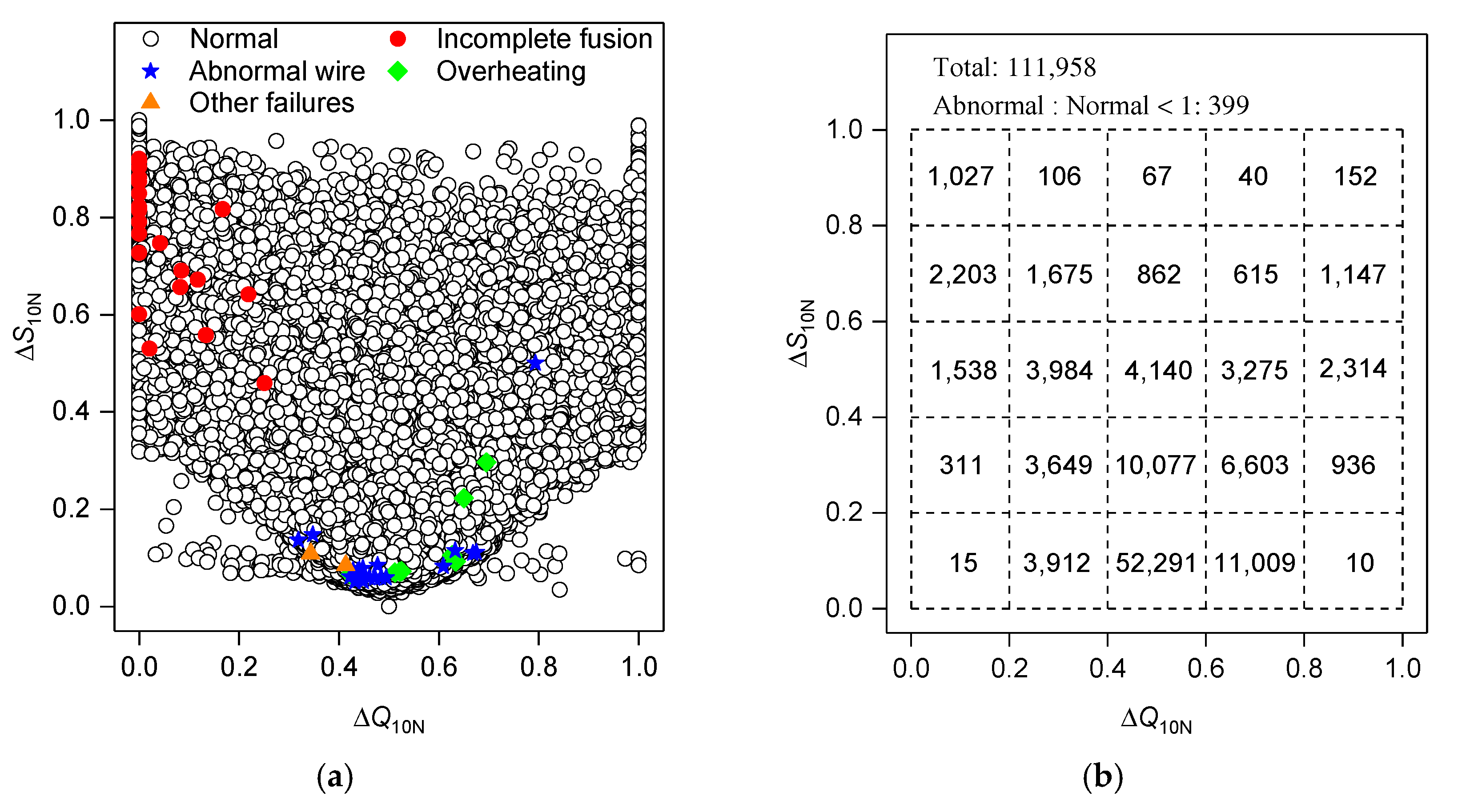
• Class imbalance and overlap exist in the quality estimation of MRSW production and require proper anomaly detection algorithms for quality monitoring.
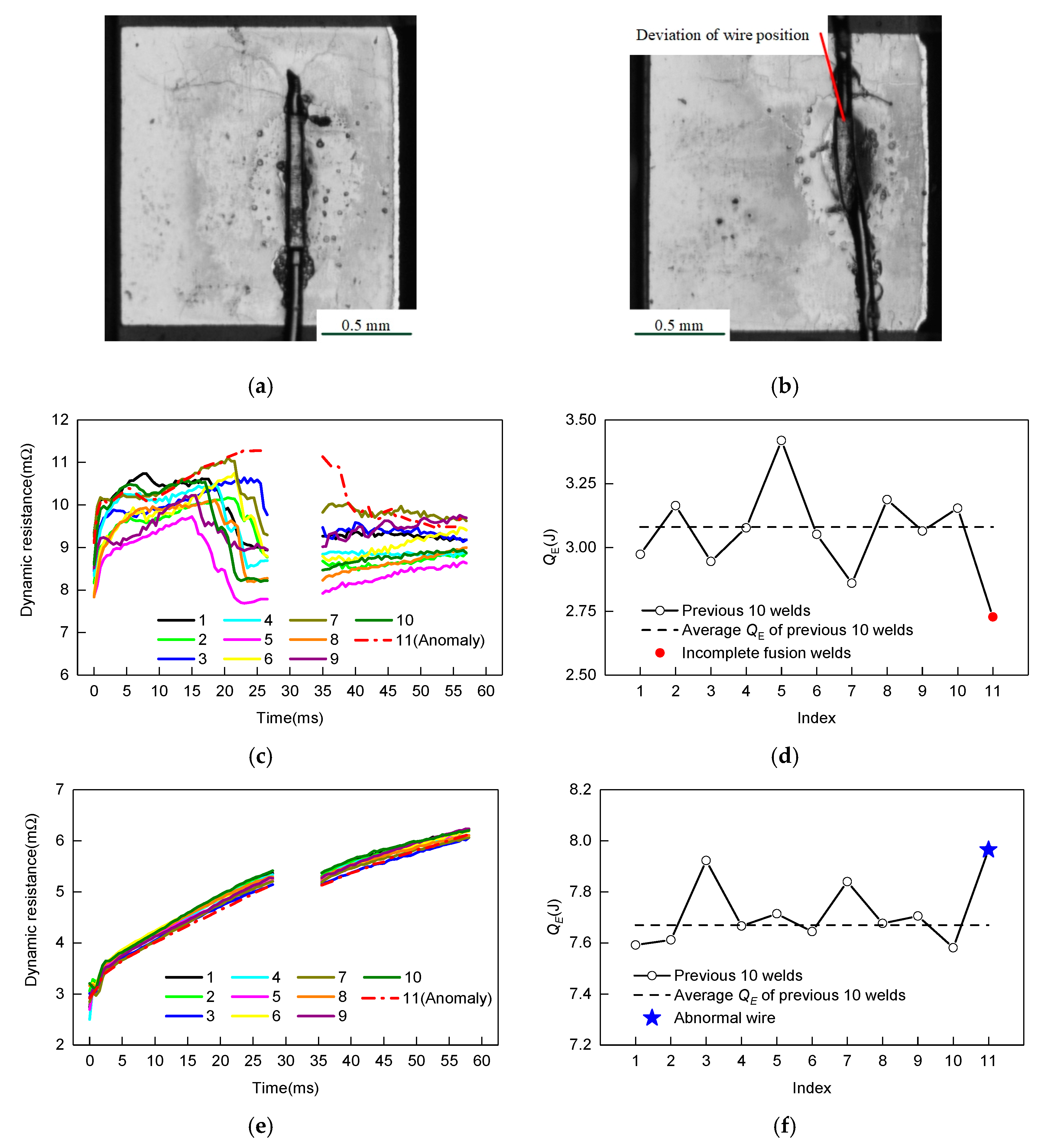
• The similarity of dynamic resistance profile and heat input compared with the previous ten welds are valid features for detecting incomplete fusion welds.
• For the classification of incomplete fusion welds and normal welds, the iForest model is a good candidate with a high AUC score of 0.9525 and high efficiency.

References

1. Yang, S.; Li, Y.; Lin, J. Stripping weld—A new technique of welding enamelled wires by resistance weld. Trans. China Weld. Inst. 2008, 29, 21–25. [Google Scholar]
2. Zeng, J.; Cao, B.; Yang, K.; Wu, M. Analysis method of electrode ignition loss state in enameled wire resistance spot welding. J. South China Univ. Technol. 2019, 47, 32–37. [Google Scholar]
3. Zhao, D.; Wang, Y.; Liang, D. Correlating variations in the dynamic power signature to nugget diameter in resistance spot welding using Kriging model. Measurement 2019, 135, 6–12. [Google Scholar] [CrossRef]
4. Wan, X.; Wang, Y.; Zhao, D. Quality evaluation in small-scale resistance spot welding by electrode voltage recognition. Sci. Technol. Weld. Join. 2016, 21, 358–365. [Google Scholar] [CrossRef]
5. Wan, X.; Wang, Y.; Zhao, D.; Huang, Y. A comparison of two types of neural network for weld quality prediction in small scale resistance spot welding. Mech. Syst. Signal. Process. 2017, 93, 634–644. [Google Scholar] [CrossRef]
6. Yue, X.; Tong, G.; Chen, F.; Ma, X.; Gao, X. Optimal welding parameters for small-scale resistance spot welding with response surface methodology. Sci. Technol. Weld. Join. 2017, 22, 143–149. [Google Scholar] [CrossRef]
7. Chen, F.; Wang, Y.; Sun, S.; Ma, Z.; Huang, X. Multi-objective optimization of mechanical quality and stability during micro resistance spot welding. Int. J. Adv. Manuf. Technol. 2019, 101, 1903–1913. [Google Scholar] [CrossRef]
8. Rikka, V.R.; Sahu, S.R.; Roy, A.; Jana, S.N.; Sivaprahasam, D.; Prakash, R. Tailoring micro resistance spot welding parameters for joining nickel tab to inner aluminium casing in a cylindrical lithium ion cell and its influence on the electrochemical performance. J. Manuf. Process. 2020, 49, 463–471. [Google Scholar] [CrossRef]
9. Zhou, K.; Yao, P. Overview of recent advances of process analysis and quality control in resistance spot welding. Mech. Syst. Signal Process. 2019, 124, 170–198. [Google Scholar] [CrossRef]
10. Xia, Y.; Li, Y.; Lou, M.; Lei, H. Recent advances and analysis of quality monitoring and control technologies for RSW. China Mech. Eng. 2020, 31, 100–125. [Google Scholar]
11. Adams, D.W.; Summerville, C.; Voss, B.M.; Jeswiet, J.; Doolan, M.C. Correlating variations in the dynamic resistance signature to weld strength in resistance spot welding using principal component analysis. J. Manuf. Sci. Eng. 2017, 139, 44502. [Google Scholar] [CrossRef]
12. Wang, X.; Zhou, J.; Yan, H.; Pang, C. Quality monitoring of spot welding with advanced signal processing and data-driven techniques. Trans. Inst. Meas. Control 2018, 40, 2291–2302. [Google Scholar] [CrossRef]
13. Chen, S.; Wu, N.; Xiao, J.; Li, T.; Lu, Z. Expulsion identification in resistance spot welding by electrode force sensing based on wavelet decomposition with multi-Indexes and BP neural networks. Appl. Sci. 2019, 9, 4028. [Google Scholar] [CrossRef] [Green Version]
14. Xing, B.; Xiao, Y.; Qin, Q. Characteristics of shunting effect in resistance spot welding in mild steel based on electrode displacement. Measurement 2018, 115, 233–242. [Google Scholar] [CrossRef] [Green Version]
15. Wen, J.; Jia, H.; Wang, C. Quality Estimation system for resistance spot welding of stainless steel. ISIJ Int. 2019, 59, 2073–2076. [Google Scholar] [CrossRef] [Green Version]
16. Gavidel, S.Z.; Lu, S.; Rickli, J.L. Performance analysis and comparison of machine learning algorithms for predicting nugget width of resistance spot welding joints. Int. J. Adv. Manuf. Technol. 2019, 105, 3779–3796. [Google Scholar] [CrossRef]
17. Amiri, N.; Farrahi, G.H.; Kashyzadeh, K.R.; Chizari, M. Applications of ultrasonic testing and machine learning methods to predict the static & fatigue behavior of spot-welded joints. J. Manuf. Process. 2020, 52, 26–34. [Google Scholar]
18. Boersch, I.; Füssel, U.; Gresch, C.; Großmann, C.; Hoffmann, B. Data mining in resistance spot welding. Int. J. Adv. Manuf. Technol. 2018, 99, 1085–1099. [Google Scholar] [CrossRef]
19. Xing, B.; Xiao, Y.; Qin, Q.; Cui, H. Quality assessment of resistance spot welding process based on dynamic resistance signal and random forest based. Int. J. Adv. Manuf. Technol. 2018, 94, 327–339. [Google Scholar] [CrossRef]
20. Pereda, M.; Santos, J.I.; Martín, O.; Galán, J.M. Direct quality prediction in resistance spot welding process: Sensitivity, specificity and predictive accuracy comparative analysis. Sci. Technol. Weld. Join. 2015, 20, 679–685. [Google Scholar] [CrossRef] [Green Version]
21. Guo, H.; Li, Y.; Shang, J.; Gu, M.; Huang, Y.; Gong, B. Learning from class-imbalanced data: Review of methods and applications. Expert Syst. Appl. 2017, 73, 220–239. [Google Scholar]
22. Liu, J.; Gu, J.; Li, H.; Carlson, K.H. Machine learning and transport simulations for groundwater anomaly detection. J. Comput. Appl. Math. 2020, 380, 112982. [Google Scholar] [CrossRef]
23. Su, Z.; Xia, Y.; Shen, Y.; Li, Y. A novel real-time measurement method for dynamic resistance signal in medium-frequency DC resistance spot welding. Meas. Sci. Technol. 2020, 31, 55011. [Google Scholar] [CrossRef]
24. Li, W.; Cerjanec, D.; Grzadzinski, G.A. A comparative study of single-phase AC and multiphase DC resistance spot welding. J. Manuf. Sci. Eng. 2005, 127, 583–589. [Google Scholar] [CrossRef]
25. Liu, F.; Ting, K.; Zhou, Z. Isolation-based anomaly detection. ACM Trans. Knowl. Discov. Data 2012, 6, 1–39. [Google Scholar] [CrossRef]
26. Schölkopf, B.; Platt, J.; Shawe-Taylor, J.; Smola, A.; Williamson, R. Estimating the Support of a high-dimensional distribution. Neural Comput. 2001, 13, 1443–1471. [Google Scholar] [CrossRef]
27. Breunig, M.; Kriegel, H.; Ng, R.; Sander, J. LOF: Identifying density-based local outliers. In Proceedings of the 2000 ACM SIGMOD–International Conference on Management of Data, Dallas, Texas, USA, 16–18 May 2000; pp. 93–104. [Google Scholar]
28. An, H.; Wang, Z.; Wang, G.; Song, Q.; Liu, F.; Zhong, C. Research on on-line monitoring of surface roughness in composite drilling and adaptive optimization of parameters. J. Mech. Eng. 2020, 56, 27–34. [Google Scholar]
29. Shi, L.; Zhou, R.; Li, J.; Wang, L.; Xu, F.; Wang, Y. New energy—Load characteristic index based on time series similarity measurement. Electr. Pow. Autom. EQ. 2019, 39, 75–81. [Google Scholar]
30. Qiu, Y.; Hu, H.; Zheng, J.; Chen, Q. On-line handwriting signature verification based on curve similarity. Syst. Eng. Electron. 2014, 36, 1016–1020. [Google Scholar]
31. Pedregosa, F.; Varoquaux, G.; Michel, V.; Thirion, B.; Grisel, O.; Blondel, M. Scikit-learn: Machine learning in python. J. Mach. Learn. Res. 2011, 12, 2825–2830. [Google Scholar]
Figure 1. Representation of MRSW: (a) schematic diagram of experimental setup; (b) a normal weld; (c) electrode and its holder; (d) main dimensions of electrode.
Applsci 10 04204 g001aApplsci 10 04204 g001b
Figure 2. Curves of voltage, current and dynamic resistance collected in a welding process.
Applsci 10 04204 g002
Figure 3. Curves of VCON, IAVE, R0 and QE during the electrode life.
Applsci 10 04204 g003
Figure 4. Schematic diagram for dynamic resistance analysis: (a) equivalent circuit; (b) electrode wear.
Applsci 10 04204 g004
Figure 5. Change of dynamic resistance profile during the electrode life.
Applsci 10 04204 g005
Figure 6. Dynamic resistance profiles: (a) Up–Up profile; (b) Up–Flat profile; (c) Up–Down profile; (d) Up&Down–Up profile; (e) Up&Down–Flat profile; (f) Up&Down–Down profile; (g) Down–Up profile; (h) Down–Flat profile; (i) Down–Down profile.
Applsci 10 04204 g006aApplsci 10 04204 g006b
Figure 7. Model construction process.
Applsci 10 04204 g007
Figure 8. Feature distribution of normal welds and abnormal welds: (a) characteristic space; (b) frequency distribution.
Applsci 10 04204 g008
Figure 9. Comparison of detection performance: (a) iForest, (b) OCSVM; (c) LOF.
Applsci 10 04204 g009aApplsci 10 04204 g009b
Figure 10. Abnormal welds and the previous 10 welds: (a) incomplete fusion weld; (b) abnormal wire weld; for incomplete fusion weld: (c) Rt profile; (d) QE; for abnormal wire weld: (e) Rt profile; (f) QE.
Applsci 10 04204 g010