Prediction of Opinion Keywords and Their Sentiment Strength Score Using Latent Space Learning Methods

Abstract

Most item-shopping websites give people the opportunity to express their thoughts and opinions on items available for purchasing. This information often includes both ratings and text reviews expressing somehow their tastes and can be used to predict their future opinions on items not yet reviewed. Whereas most recommendation systems have focused exclusively on ranking the items based on rating predictions or user-modeling approaches, we propose an adapted recommendation system based on the prediction of opinion keywords assigned to different item characteristics and their sentiment strength scores. This proposal makes use of natural language processing (NLP) tools for analyzing the text reviews and is based on the assumption that there exist common user tastes which can be represented by latent review topics models. This approach has two main advantages: is able to predict interpretable textual keywords and its associated sentiment (positive/negative) which will help to elaborate a more precise recommendation and justify it, and allows the use of different dictionary sizes to balance performance and user opinion interpretability. To prove the feasibility of the adapted recommendation system, we have tested the capabilities of our method to predict the sentiment strength score of item characteristics not previously reviewed. The experimental results have been performed with real datasets and the obtained F1 score ranges from 66% to 77% depending on the dataset used. Moreover, the results show that the method can generalize well and can be applied to combined domain independent datasets.

1. Introduction

User-modeling and personalization has been the cornerstone of many of the new services and products in the high-tech industry. The personalization of contents reduces information overload and improves both efficiency of the marketing process and the user’s overall satisfaction. This is especially relevant in e-commerce web sites—e.g., Amazon- and Social Networking Services (SNSs) where users may read published opinions to gather a first impression on an item before purchasing it and express their opinions on products they like or dislike. Recommender systems use this information transforming the way users interact and discover products on the web. When users assess products, the website models how the assessments are done to recommend new products they may be interested in [1], or to identify users of similar taste [2]. Most existing recommendation systems fit into one of the following two categories: (i) content-based recommendation or (ii) collaborative filtering (CF) systems [3].

The first approach defines the users profile that best represents all the gathered personal information (such as tags, keywords, text comments, and likes/dislikes [4]) and recommends items based on each individual characteristics. These recommendations are then generated by comparing items with user profiles [4]. The main benefit of this approach is the simplicity and ease of interpretation of the recommendations it provides. One of its main drawbacks is the fact that it ignores user opinions on different products, taking only their preferences into account. Figure 1 shows the metadata of a real text review that includes the user’s opinion. There are several works that try to solve this limitation by including the text features of the user’s reviews (e.g., frequencies of occurrence of words) into the model. In [5] the authors incorporate reviews, items, and text features into a three-dimensional tensor description to unveil the different sentiment effects that arise when the same word is used by different users in ranking different items. These improvements lead to better ranking predictions when compared to previous models. Also, ref. [6] presents an extension of the user-$kNN$ algorithm that uses the similarities between text reviews to gather the similarity between users, outperforming the conventional algorithms that only use the ratings as inputs.

On the other hand, the CF category has achieved the most successful results as shown in the Netflix Prize Challenge [7,8]. This method uses the similarities among users to discover the latent model which best describes them and retrieves predicted rankings for specific items. Some modifications have been later proposed to properly address the negative latent factors [9,10] as well as to gain interpretability [11]. In this last reference, authors present a hidden factor model to understand why any two users may agree when reviewing a movie yet disagree when reviewing another: The fact that users may have similar preferences towards one genre, but opposite preferences for another turns out to be of primary importance in this context. These same authors also propose in [1] the use of the latent factors to achieve a better understanding of the connection between the rating dimensions and the intrinsic features of users and their tastes.

During the last decade, the proliferation of social media has gone hand in hand with the analysis of user opinions and sentiments [12], which has been applied successfully in a variety of fields such as social networks [13] or movies [14]. In [15] authors use text reviews to describe user interests and sentiments, hence improving the results obtained in the prediction of the ratings. These text reviews are also used [16,17] to guide the learned latent space by combining content-based filtering with collaborative filtering techniques. However, being capable of predicting the opinion or sentiment associated with non-existent reviews remains an open question that deserves further attention [18]. This article in particular focuses on improving the current recommendation systems by predicting the sentiment strength scores for a series of opinion keywords that describe each item.

This can be illustrated with the following text review (see Figure 1): “These are probably the best sounding guitar strings without breaking the bank. I have made them last up to 2 months …still obtaining decent sound”. Its overall rating score is 4 and a natural language processing analysis provides information about what the most representative opinion-words of that review are (see Section 2 for more detail on this analysis). Here, the proposed dictionary for the musical instruments domain that this review belongs to is composed by the words {feel; guitar; string; price; quality; sound; string; tone} and the extracted sentiment for opinion keywords subject to prediction in the review are {guitar (+1.2); string (+0.3); sound (+2)} (sentiment strength scores are enclosed in brackets). Similarly, the sentiment keywords for a second review example “These strings sound great. I love the sustained bright tone. They work well with my cedar top guitar. Easy on the fingers too” (with an overall score of 5) are {string (+4); cedar (+1); finger (+2); guitar (+5); tone (+3)}.

The previous examples exemplify the usefulness of the prediction of sentiment strength scores in this context: They provide insights into the reasons why a user would like or dislike a product (recommendation explanation). These predictions are highly valuable for personalized product recommendation since they explain why the recommendation system ’thinks’ users would like the recommended product. They also lead to a double-check verification on the assumptions made by the system according to the user needs, making the systems more robust. Furthermore, it is well known that emotions are important factors that influence overall human effectiveness including rational tasks such as reasoning, decision making, communication, and interaction [19]. In this context, the prediction of sentiment keywords can be a middle step towards the prediction of users emotions (e.g., using six basic Ekman’s emotions [20,21]) associated with the item under recommendation [22,23].

Our main contribution is to propose and describe a model that combines the use of latent spaces—connected with user tastes and product features, sentiment language analysis, and matrix factorization techniques to predict user opinions. Concretely, we generate a distinct vocabulary for each item based on previously submitted reviews and will predict the sentiment strength a user would give to each opinion-word in the vocabulary. This article provides an extensive analysis (both qualitative and quantitative) showing the capabilities of the proposed method on the Amazon benchmark dataset [24]. This gives us a better understanding of the main reasons why a user would like or dislike a product.

We would like to stress that we are not interested in predicting the opinion-words themselves, but the strength of the sentiment associated with the item characteristics. Our approach naturally extends previous works [25,26] assuming the existence of a latent space that accurately represents the user interests and tastes [11]. The approach is based on a two-step process: (i) Setting up the opinion dictionary associated with the Amazon dataset under study, and (ii) Prediction of the sentiment scores that users would assign to some keywords that describe the item should they have the opportunity to review it, based on the hidden dimensions that represent their tastes and interests. It is well known that the input matrix sparsity (which is a sub-problem of the cold-start problem) of this type of datasets is typically very large (≈99%) [27]. This explains the need to reach a trade-off between the maximum number of opinion keywords which are desirable to predict without enlarging the sparsity too much, and the minimum amount to be predicted in order to ensure a minimal functionality.

Related Work

Incorporating the latent factors associated with users has been proven to be very useful to design effective algorithms in ranking and recommendation systems [8,28,29]. These works are based on the idea of factorizing a matrix to linearly reduce the dimensionality of the problem and extract some commonalities that may be implicit in the data under analysis. Most of the techniques used the Singular Value Decomposition (SVD) to perform the matrix decomposition or its high-order SVD version for tensors. One common problem of this type of solution is missing data that may be solve using the average ratings for an item. However, this solution is only possible if second step is adopted to learn the association between the new created features and the ranking (e.g., using item-item or user-user collaborative filtering approach individually). Another approach is to use Alternative Least Squares [30] to minimize the difference between the original data and the projected that consider only non-missing values. Moreover, the large sparsity of the data under analysis can be up to 99% for datasets such as Amazon product review undermining the capabilities of this type of learning methods based on matrix decomposition. Some alternative works propose the use of specific regularization parameters to minimize this effect [28].

In our field of recommendation explanation, the sparsity is increased because we not only use the rating value for each product but the opinionated dictionary for each one. It has been demonstrated that this system’s ability to explain why items are suggested and a good explanation interface could help inspire user trust and satisfaction [31,32]. This human-centered approach distinguishes from raw sentiment analysis by using the second as input for the recommendation system. Thereof the system explains why the products are recommended by using the sentiment/opinion-words and provides transparency, sense of control of the system, and improves user overall satisfaction [33].

In this context, we postulate that given the largeness and sparsity training dataset, CF techniques should be used to predict a set of sentiment strength scores associated with a list of opinion keywords that essentially compose the user’s opinion on an item he did not review yet. Reviews contain opinions, topical and emotional information that gives clues about what the writer possibly wants to transmit [34]. The first studies distinguished between positive (favorable) and negative (unfavorable) opinions about a topic [35,36], and the extracted sentiments were later used to infer unknown ratings [22,37]. However, none of these works aimed to predict the texts reviews themselves, nor the sentiments of the lists of opinion keywords that characterize them. Moreover, we assume that this user’s opinion may be described as a set of features in a so-called latent space. There are previous works that support this assumption [11] indicating that there exist a latent space that represents the user interest and tastes although the authors did not provide a model to predict the sentiment score of the item characteristics.

The rest of the article is organized as follows: Section 2 contains the description of the opinion prediction model and our overall approach. Section 3 describes the experiments we conducted to test the implemented model, and Section 4 includes the obtained results. Finally, Section 5 presents the conclusions and some insights into future work.

2. Latent Space Based Learning

The first step toward the creation of a model to predict the sentiment score of previously unseen item characteristics is to define a specific vocabulary for each product, since user overall opinion orientations are based on the opinion-words they use to describe the items.

2.1. Opinion Dictionary Generation

Opinion-words are often referred to as sentiments in the literature and categorized as:

• Rational sentiments, namely “rational reasoning, tangible beliefs, and utilitarian attitudes” [38]. An example of this category is given by the sentence ‘This camera is good”, which does not involve emotions like happiness at all. In this case, the opinion-word (the adjective “good”) fully reveals the user’s opinion on the phone.
• Emotional sentiments, described in [12] as “entities that go deep into people’s psychological states of mind”. For example, consider the sentence “I trust this camera”. Here, the opinion-word “trust” clearly conveys the emotional state of the writer.

An opinion dictionary contains both keywords that represents item characteristics and the sentiment strength scores associated with them. As with [39,40], these scores are determined using a word-similarity-based method that assumes that similar meanings imply similar sentiments, and then weighted based on the SentiWordnet sentiment corpus [41].

Table 1. Sentiment Analysis Example.

	Opinion Keyword	Sentiment Text	Score
Opinion 1	“phone”	“awesome”	+4.0
Opinion 2	“phone”	“much too expensive”	−5.4
Opinion 3	“screen”	“not big”	−1.0

shows an example of the obtained sentiment scores associated with several item characteristics of a phone review.

The dictionary can be of constant length—common to all products—containing the most commonly used opinion-words in the whole review dataset [42], or as proposed of variable length solving the problems of: (i) using a large set of words that are not shared by different products and thereof introducing unnecessary sparsity in the input matrix, (ii) this same increase on sparsity worsens to some extent the prediction capabilities of the algorithm, and (iii) the only use of opinion-words as vocabulary allows the overall opinion prediction for a product but not for the sentiment associated with its characteristics. Since different products have truly different features, we must consider a distinctive set of opinion-words for each one of them, reducing the number of features and the sparsity of the input matrix.

In this context, every user review of a particular item reduces to a (possibly sparse) array of sentiment scores associated with the item vocabulary. If an opinion keyword occurs more than once in the review, its final score is calculated simply as an average.

These feature vectors were obtained using a solution similar to that described in [43] (we used the NTL services graciously provided to us by www.bibtex.com), that carries out sentiment analysis at the sentence level and can detect as many opinions as contained in a sentence. This analysis identifies the opinion keyword (the what) for each opinion sentence and calculates a numerical sentiment strength score for it based on its associated sentiment text (the why). Also, the analysis enables us to syntactically analyze the texts and extract the simple (e.g., ‘guitar’) and compound (e.g., ‘quality_interface’) opinion keywords to include in the feature vectors. To further elaborate one of the examples provided above, three distinct sentiment opinions may be extracted from the review “This phone is awesome, but it was much too expensive and the screen is not big enough”, namely:

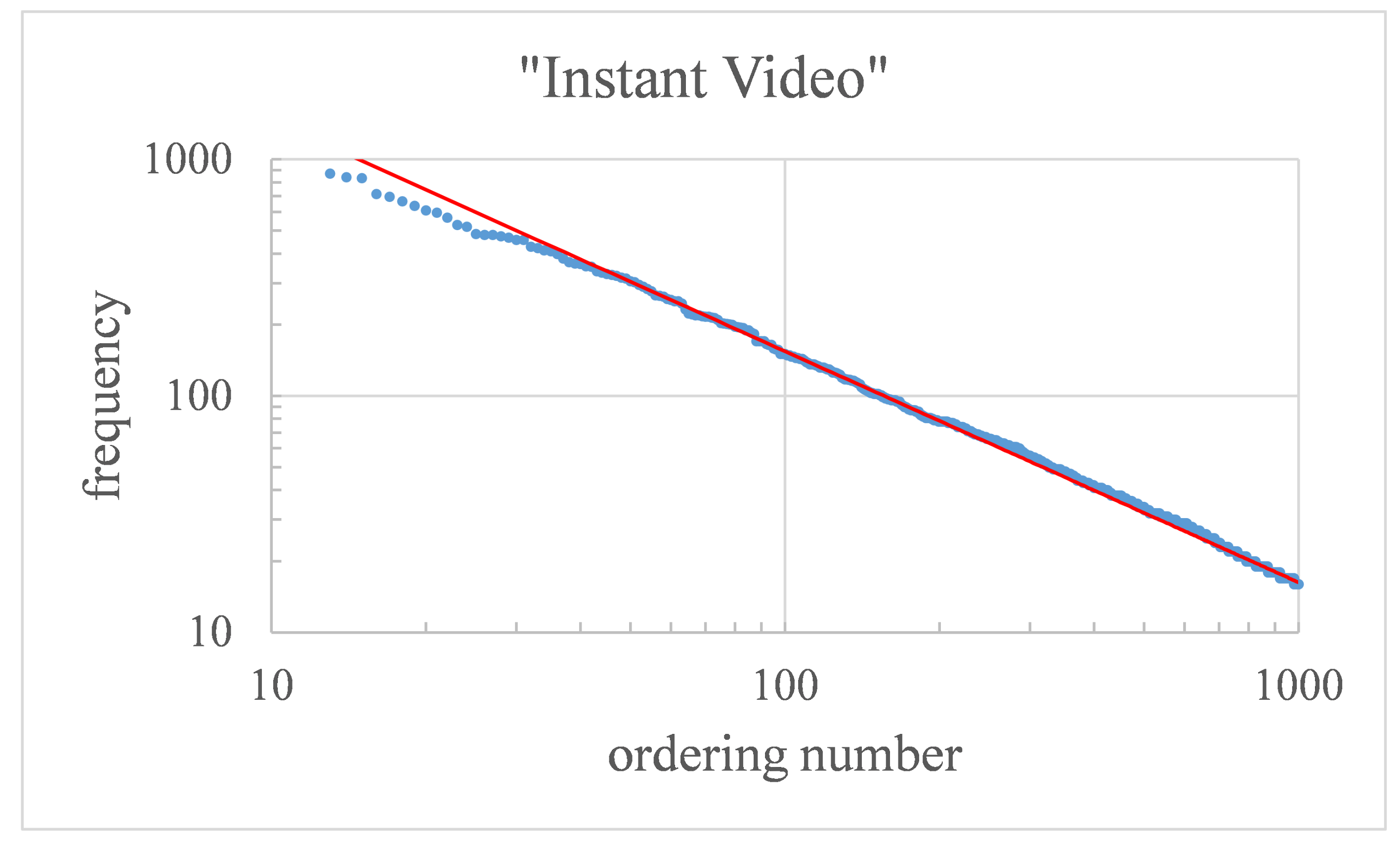
It is worth noting that we validated the generated vocabularies verifying that they accomplish with the frequency distribution that characterizes the majority of natural languages and is defined by a power law distribution known as Zipf’s law [44,45]. This validation is shown in Figure 2, where the frequency of occurrence of the opinion keywords in the Amazon’s “Instant Video” dataset is plotted as a function of its ordering number n. The distribution that best fits the data is $f=C{n}^a$ with $a=-0.953\pm 0.001$.

2.2. Notation and Input Matrix

In this section, we explain the opinion prediction model based on tensor factorization in full detail, and introduce the terminology and notation used throughout this article. One of the challenges in the design of the model lays in the use of a vocabulary rich enough as to characterize the user viewpoints, but not too large (notice that without any filtering the number of possible words obtained for the used datasets is ≈10.000) as to impede numerical computations or the learning capabilities. The main difficulty in dealing with such models does not lie on its computational aspects however, but in the sparsity and noise of the data. This sparsity engages critically with the cold-start problem in recommendation systems. A typical online shopping website with SNS capabilities provides, for the purposes of this article, N users writing reviews on a set of M items. Generally, a given user will have scored and reviewed only a subset of these M items, thus making the website’s database highly sparse.

Let S denote the set of user-item pairs $\left\{\right(u,i\left)\right|u=1,\dots ,N;i=1,\dots ,M\}$ for which written reviews do exist and let ${\mathbf{t}}_{ui}$ be their associated feature vectors. Our information domain consists therefore of triples of the form $(u,i,{\mathbf{t}}_{ui})$. In general, each item is described by a different set of opinion topics (keywords) of size $D_i$. The ${\mathbf{t}}_{ui}\in {\mathbb{R}}^{D_i}$ vector is populated with the sentiment strength scores $s_{uij}\in (-\infty ,+\infty )$ ($j=1,\dots ,D_i$) given to the topics in the $(u,i)$-th review.

The website’s 2-dimensional input matrix $\mathbf{R}:=[{\mathbf{R}}_0{\mathbf{R}}_1\cdots {\mathbf{R}}_M]$ is set up by concatenating the $N\times D_i$ sparse matrices ${\mathbf{R}}_i$ containing the reviews for the $i=1,\dots ,M$ products. Thus, $\mathbf{R}\in {\mathbb{R}}^{N\times D}$, where $D:={\sum }_i{D}_i$ denotes the sum of the vocabulary sizes for the M products.

Let $s_{ij,\min }$ and $s_{ij,\max }$ be, respectively, the minimum and maximum sentiment scores contained in the $({\sum }_1^i{D}_k+j)$-th column of the input matrix $\mathbf{R}$. Each $s_{uij}$ entry is then replaced by its normalized value ${\overline{s}}_{uij}\in [-1,1]$ defined as

$${\overline{s}}_{uij}:=\left\{\begin{array}{ccc}{s}_{uij}/\left|s_{ij,\min }\right|\hfill & \mathrm{if}\hfill & s_{uij}<0\hfill \\ s_{uij}/s_{ij,\max }\hfill & \mathrm{if}\hfill & s_{uij}\ge 0\hfill \end{array}\right..$$

Please note that two different normalization scales are used depending on the entry sign to prevent turning positive scores into negative ones and vice versa. In what follows, normalized scores will be denoted simply by $s_{uij}$.

Table 2. Notation.

Symbol	Description
u	user, reviewer
N	total number of users
i	item, product
M	total number of items
S	set of $(u,i)$ pairs of existing reviews
${\mathbf{t}}_{ui}$	u-th user review (‘document’) on i-th item
$t_{ij}$	j-th sentiment keyword for the i-th item
$s_{uij}$	normalized sentiment strength score for the j-th keyword in ${\mathbf{t}}_{ui}$
${\widehat{s}}_{uij}$	predicted ALS-generated sentiment score
$D_i$	vocabulary size of the i-th product dictionary
D	sum ${\sum }_i^M{D}_i$ of all dictionary lengths
$\mathbf{R}$	input matrix in ${\mathbb{R}}^{N\times D}$
K	rank, number of latent dimensions
$\lambda$	ALS’s regularization parameter
$n_{\mathrm{iter}}$	number of ALS iterations

summarizes the terminology and notation used in this article. See also Figure 3 for further clarification.

2.3. Prediction Model

We aim to obtain a prediction model that minimizes the reconstruction error ${\sum }_{uij}{\left(s_{uij}-{\widehat{s}}_{uij}\right)}^2$ of the sentiment strength scores over all users, items, and opinion-words. For minimizing the above expression our model uses the Alternating Least Squares (ALS) method to reconstruct user opinions—that is, ${\mathbf{t}}_{ui}$ vectors—not included in S. This factorization collects patterns of taste among similar reviewers generating automatic predictions for a given user.

Specifically, we subject the input matrix $\mathbf{R}\in {\mathbb{R}}^{N\times D}$ to an ALS factorization [30] of the form $\mathbf{R}\approx \mathbf{P}{\mathbf{Q}}^{\mathrm{T}}$ in order to estimate the missing reviews. Here, $\mathbf{P}\in {\mathbb{R}}^{N\times K}$ and $\mathbf{Q}\in {\mathbb{R}}^{D\times K}$, where $K\in \mathbb{N}$ is the number of latent factors or features [8]—a predefined constant typically of the order of ten. Any sentiment score $s_{uij}$ can then be approximated by the scalar product ${\widehat{s}}_{uij}:={\mathbf{p}}_u^{\mathrm{T}}{\mathbf{q}}_{ij}$ (recall that ${\widehat{s}}_{uij}$ is the prediction), where ${\mathbf{p}}_u\in {\mathbb{R}}^{K\times 1}$ is the u-th row of $\mathbf{P}$ and ${\mathbf{q}}_{ij}\in {\mathbb{R}}^{K\times 1}$ the $({\sum }_1^i{D}_k+j)$-th row of $\mathbf{Q}$. The procedure monotonically minimizes the following quadratic loss function until convergence is reached

$$\langle \mathbf{P},\mathbf{Q}\rangle :={\arg \min }_{\mathbf{P},\mathbf{Q}}\sum _{(u,i)\in S}\left(\lambda {\mathbf{p}}_u^{\mathrm{T}}{\mathbf{p}}_u+\sum _{j=1}^{D_i}\left({\epsilon }_{uij}^2+\lambda {\mathbf{q}}_{ij}^{\mathrm{T}}{\mathbf{q}}_{ij}\right)\right),$$

where ${\epsilon }_{uij}:=s_{uij}-{\widehat{s}}_{uij}$. Here, $\lambda$ denotes the regularization parameter that prevents overfitting and plays a crucial role in balancing the training error and the size of the solution (see Section 4 for further details).

3. Experiments

We tested our model using different Amazon datasets (http://jmcauley.ucsd.edu/data/amazon/) as explained in Section 2.1 and Section 2.2. We performed an exhaustive number of analysis in order to optimize the internal parameters of the model—namely K, $\lambda$, and the number $n_{\mathrm{iter}}$ of ALS iterations—for comparative and validation purposes, providing the updated results of the global performance.

3.1. Dataset

To conduct our experiments, we chose four 5-core version Amazon datasets [24] of increasing size—it basically doubles from one dataset to the next—and similar characteristics—especially regarding their population ratios between positive and negative sentiment scores. These datasets belong to different domains: Musical instruments, automotive, instant video, and digital music, and the union of these datasets is also used to measure generalization capabilities of our method.

Table 3. Amazon dataset features.

	Reviews	Users	Products	Number of Entries	Ratio of Positive vs. Negative/neutral	Sparsity
Musical Instruments	10,261	1429	900	41,942/6158	87.1%	97.5%
Automotive	20,473	2929	1835	75,917/9835	82.0%	98.9%
Instant Video	37,126	5129	1685	165,989/34,802	78.8%	97.8%
Digital Music	64,706	5536	3568	483,232/91,801	77.1%	99.88%
Combined datasets	132,566	14,809	7988	767,080/142,689	78.3%	99.95%

lists the datasets and summarizes their main features.

To reduce sparsity we selected those records with at least five reviews for each item and user, and also a constraint of minimum three occurrences $f_{\min }=3$ was set for the inclusion of a word in the opinion dictionaries to retain only the most relevant opinion keywords while keeping the complexity of the problem manageable. Thus, only a term that occurred at least three times in the subset of reviews for an item was considered relevant, and hence included in that item dictionary. Recall that this same term it may or may not be present in other item dictionaries. Table 3 shows the number of entries before and after this threshold was applied (see its fourth column).

Table 4. Some items’ dictionaries.

Text Review ID	Extracted Opinion Dictionaries
B00CCOBOI4 (Automotive)	3_month, car, instruction, job, layer, paint, problem, product, a result, stuff, surface, thing
B0002CZUUG (Musical Instruments)	action, finish, guitar, neck, pickup, sound, review, string, quality, way
B003VWJ2K8 (Musical Instruments)	battery, buy, clip, deal, display, design, color, guitar, head, item, job, price, problem, product, purchase,
	quality, result, Snark, Snark_SN-1, spot, string, thing, time, tune, tuner, tuning, use, value, work

also shows some of the vocabularies generated in this way.

3.2. Technical Aspects

The implemented algorithms are scalable and may be executed over large datasets by using any Hadoop-based cluster or distributed computational infrastructure. Our numerical computations were performed in a distributed system of 2 executors with 16 cores and 256GB RAM on a Hadoop cluster with a total of 2.8TB RAM, 412 cores, and 256GB HDFS. We implemented our codes using the Python 3.5 programming language and the collaborative filtering RDD-based algorithms provided by Apache Spark, both being solutions of well-known efficiency, robustness, and usability.

3.3. Experimental Design

We have performed five experiments related with each one of the datasets (musical instruments, automotive, instant video, and digital music) to test the learning capabilities of the proposed method. Moreover, we performed an additional experiment to test the generalization capabilities by joining the fours datasets to create a bigger one that is domain independent. This implies that the vocabulary is global, and the goal is to test how large is the difference between domain dependent and independent approaches.

We evaluated our model performance and set the ALS parameters $(K,\lambda ,n_{\mathrm{iter}})$ for each dataset by means of a 5-fold cross-validation. The performance was measured by analyzing the Mean Squared Error (MSE), accuracy, $F_1$-score, precision, recall and Area Under the Curve (AUC) metrics. The MSE measures the error obtained by the prediction model during the cross-validated learning process and has been used to prevent overfitting. The accuracy provides an overall success criterion ($\frac{TruePositive+TrueNegative}{Totalpopulation}$) without considering the data distribution. The precision ($\frac{TruePositive}{PredictedPositive}$) provides the percentage of the correctly predicted opinion keywords and their sentiment. Recall metric ($\frac{TruePositive}{ConditionPositive}$) provides the percentage of the correctly detected opinion keywords and their sentiment, and the $F_1$-score ($2\frac{Precision*Recall}{Precision+Recall}$) has been used as application metric success because it is equally important to detect an opinion keyword that exists than not to say that exists when is not. Finally, the AUC metric has been used to verify that the obtained model behavior is independent of the data distribution.

To obtain the input matrix S we first processed the reviews using NLP and the opinion dictionary generation method explained in Section 2.1 and then obtained the optimal parameters by conducting the following experiments:

• Combined analysis of $\lambda \in \{0.01,0.02,0.03,0.04,0.05,0.07,0.1,0.2,0.3,0.4,0.5,0.7\}$ and $K\in \{5,10,20,50,100,200\}$ parameters to probe whether they can be set independently for each dataset.
• Analysis of the influence of the optimal K value on the model performance for different datasets and $\lambda$ values.
• Analysis of the number of iterations needed until convergence is reached.

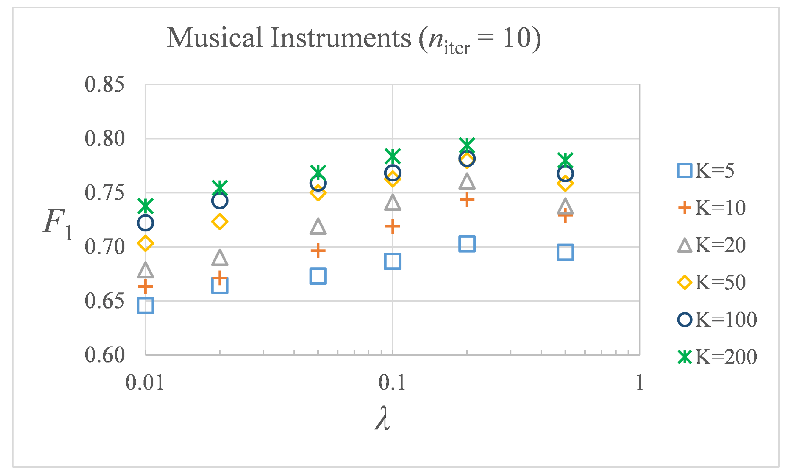
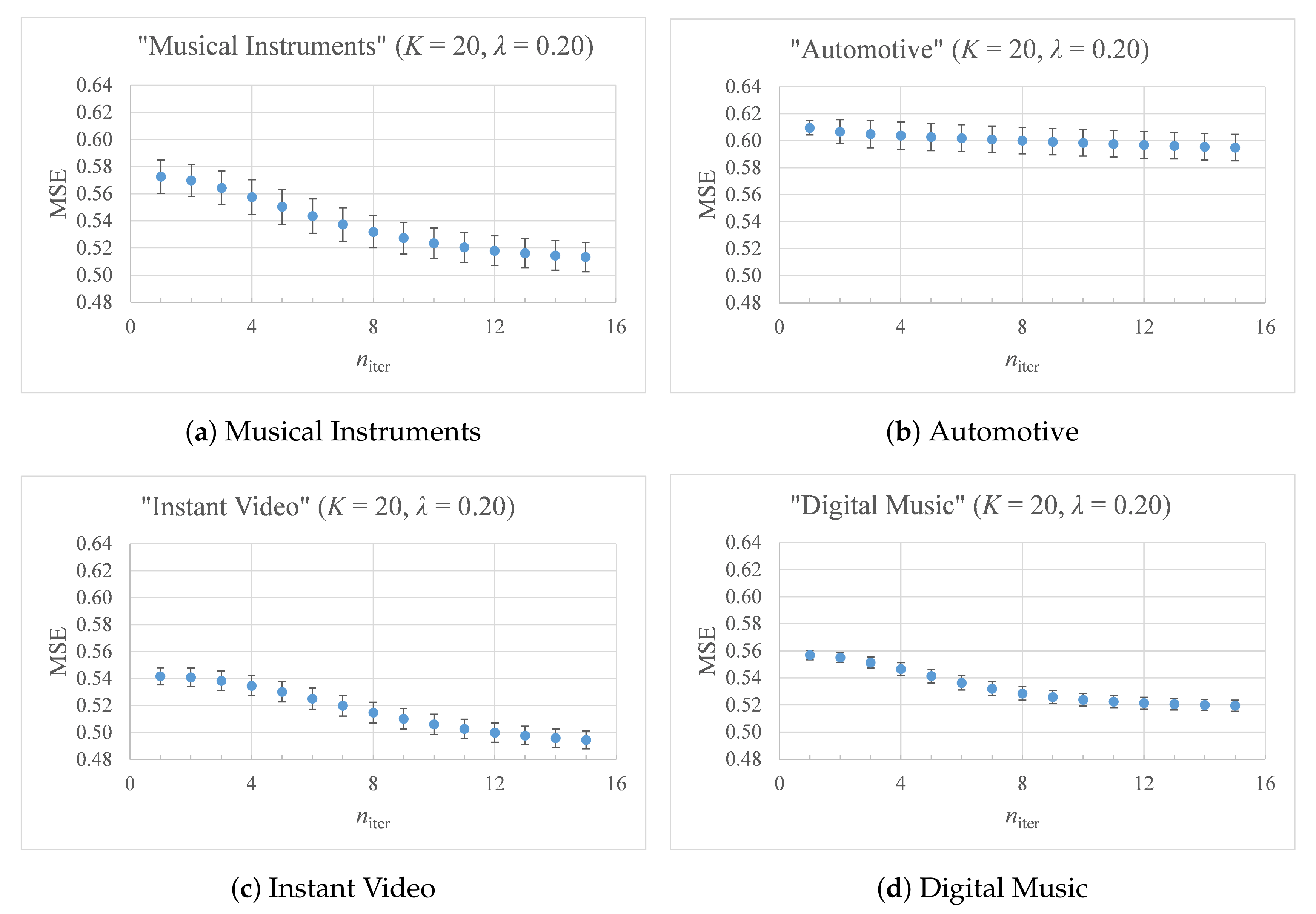
We want to point out that despite the use of a cluster, it was still very time-consuming to perform an exhaustive trial and error for all the possible parameter combinations of the model. Hence, when deciding on a choice for K and $n_{\mathrm{iter}}$, we had to reach a compromise between the model error and the running time of the ALS method, which is proportional to $K^3$ [46]. For this purpose, we followed an incremental approach. We first corroborate that $\lambda$ and K are, in effect, unrelated parameters in our model (see Figure 4. Indeed, the $F_1$-score versus $\lambda$ curves have the same shape for different values of K, and all of them attain their maxima at the same $\lambda$. Consequently, $\lambda$ and K may be optimized independently. Note also that the vertical distance between $F_1$-scores for a given $\lambda$ is negligible for sufficiently large values of K (the percentage MSE error reduces to less than $0.5\%$ from this value forward) and therefore we use $K=20$ throughout this article. Then, we evaluated the optimal number of iterations until convergence of the ALS method. Figure 5 shows the MSE values relative to the number $n_{\mathrm{iter}}$ of ALS iterations for $\lambda =0.2$ and $K=20$. The number of iterations necessary for the model convergence is expected to depend mostly on the size of the dataset (the higher $n_{\mathrm{iter}}$, the lower MSE once $\lambda$ and K have been set in advance). Curves converge almost asymptotically towards low error values, reaching a plateau in which the model performance is virtually constant and the best learning results are attained. A value of $n_{\mathrm{iter}}=10$ seems to be a suitable number of iterations for subsequent experiments. The last set of performed experiments to configure the parameters of our model measure the $F_1$ and AUC metrics as functions of $\lambda$ in order to obtain the optimal regularization parameter for each dataset. Both Figure 6 and Figure 7 show similar behavior—particularly, they attain their corresponding maxima at the same $\lambda$, although AUC has larger standard deviations for some datasets—see, for instance, Figure 7a). When needed, the $F_1$ curves were used for clarification purposes, helping us to point out the optimal K rank. The obtained optimal parameters are $K=20, \lambda =0.2,$ and $n_{iter}=10$.

4. Results

To extract the user’ opinion (positive or neutral/negative) for the different item characteristics, once the ALS factorization of the input matrix is completed, we proceed to categorize the output data (i.e., predicted ${\widehat{s}}_{uij}$ sentiment scores) into two classes depending on whether the opinion for a specific topic is positive (${\widehat{s}}_{uij}>0$ class), or negative or neutral (${\widehat{s}}_{uij}\le 0$ class).

The model performance is assessed by means of $2\times 2$ confusion matrices and their associated metrics: accuracy, F1-Score, precision and Recall; that measures the percentage of the correctly predicted values. These metrics provide insights on result goodness but, due to the unbalanced number of positive/negative samples ratio and the equally importance of misleading a positive or negative prediction, the AUC as performance metric is recommended. Recall that AUC considers the relationship between the sensitivity (true positive rate) and fall-out (false positive rate) being a more robust metric for our case.

The final results of the above described optimal model are shown in

Table 5. Model performance for several Amazon datasets ($K=20$, $\lambda =0.2$, $n_{\mathrm{iter}}=10$). Values enclosed in parenthesis show the standard deviation at the least significant figure.

	${\mathit{F}}_1$-Score	Accuracy	Precision	Recall	AUC
Musical Instruments	0.77(2)	0.64(3)	0.87(1)	0.68(4)	0.51(1)
Automotive	0.667(8)	0.544(8)	0.826(9)	0.56(1)	0.516(9)
Instant Video	0.730(4)	0.615(4)	0.814(7)	0.663(7)	0.551(4)
Digital Music	0.728(8)	0.611(8)	0.790(2)	0.67(1)	0.54(1)
Combined datasets	0.726(5)	0.609(5)	0.801(2)	0.664(9)	0.537(3)

. It can be observed that there exists consistency among the metrics for the different datasets. Overall, smaller datasets perform slightly better than larger ones in terms of $F_1$, accuracy, precision, and recall metrics. The reason for this behavior is two-fold: First, the input matrix sparsity increases with the dataset size, which hinders the learning process. Second, the positive score population is also patently larger in smaller datasets (with a maximum at 87.1%), dominating over the negative/neutral class. This does not undermine the model foundation, however: This positive-negative score ratio is observed to be shared by most Amazon datasets and, in any case, we are equally interested in both classes of opinions.

It is in this sense, the AUC metric gives equal importance to positive and negative/neutral classes resulting in a more suitable metric to measure the model prediction capabilities from an application perspective. Its best results are now obtained for the larger datasets and it is also worth highlighting the relatively large AUC achieved for the combined dataset. These results follow from the existence of user complementary information in intersecting datasets.

To be certain about the significance of the results using the AUC metric, it must be noticed that any random binary classifier is expected to yield an average $\mathrm{AUC}$ of $1/2$. All our experiments were significantly better than $0.500$ compared with the Monte Carlo simulated frequency distribution of the computed AUC over our datasets. The distribution peaks at $0.500$, as expected, and is relatively narrow, with approximately $99\%$ of all repeated measurements lower than $0.507$. This demonstrates a negligible probability of generating the true experimental value of $0.551$ by chance (see Table 5) and the significance of the improvement obtained with our method.

Finally, it is worth discussing an actual review instance of the full experimental procedure to spot its strengths and aspects that call for improvement. Such an example is shown in

Table 6. A detailed example of the results obtained showing the original unprocessed review and the predicted sentiment scores for each opinion keyword in the product dictionary. Amazon dataset: ‘Musical Instruments’, product ID: B0018TIADQ, user ID: A15BHBF0L0HV1F.

	Opinion		Sentiment Strength Score
Opinions in the Review	Topic	Sentiment Text	Unprocessed	Normalized	Predicted
1. “There isn’t much to get excited about in a guitar stand,”	-	-	-	-	-
2. “however, it does its job and the price was right.”	“price”	“right”	$2.000$	$0.250$	$0.272$
3. “I purchased four and they were all delivered on time.”	-	-	-	-	-
4. “Each adjusted to, and held, its guitar securely.”	“guitar”	“securely”	$2.000$	$0.500$	$0.403$
5. “I have found the stand to be very stable.”	“stand”	“very, stable”	$4.000$	$0.500$	$0.123$
6. “The welds seem secure ad the materiel heavy enough to do the job.”	“weld”	“secure”	$2.000$	-	-
7. “My music teacher has a similar stand which cost him 4x as much.”	-	-	-	-	-
8. “It does not appear to be of better quality.”	“quality”	“better”	$3.000$	-	-

. This particular review contains eight syntactic structures which are shown independently (notice that the NLP analysis for obtaining the opinion keywords and its sentiment is performed at sentence level). Our sentiment analysis service detects five topics/opinion keywords and assesses them with unprocessed sentiment strength scores (third column). The frequencies of occurrence of two of these opinion keywords, namely ‘weld’ (at row 6) and ‘quality’ (at row 8), are lower than the threshold frequency explained in Section 3.1, and are therefore discarded. The remaining three entries, normalized as explained in Section 2.2, were originally positive and therefore successfully predicted as such by our binary classifier.

5. Conclusions and Future Work

The fundamental hypothesis behind our model is that any user review encodes preferences, emotions and tastes that may be captured by latent factors that are common to similar users. These emotions are then open to be predicted as opinion keywords containing a sentiment strength score of item characteristics.

In our model, every product has its own vocabulary, which is rich enough as to allow users to be expressive, but not too large as to increase the data sparsity—which burdens the learning process. A careful choice of opinion keywords for the domains under analysis proves to be crucial if we want to avoid topics of low descriptive value. We want to highlight that this article is, to the best of our knowledge, the first study that tries to predict the user’s textual opinion by means of predicting the sentiment strength scores for item characteristics. The obtained results prove that the proposed model is indeed able to learn despite they still are far away to be considered in real environments. Nonetheless, the model is still open to improvements and we expect it to be useful as a baseline for comparative purposes in SNS solutions.

Our future work includes using larger datasets to verify the generalization capabilities of the system, since our experiments show a consistent reduction of MSE values with their size at least in domain dependent scenarios, as well as reduce the sparsity of the dataset by using the current prediction system (which has an accuracy above 60%) to generate new samples and populate incrementally a new dataset following a best-candidate sampling. We expect that this reduction of sparsity will improve the generalization capabilities of the system.

References

1. McAuley, J.; Leskovec, J. From amateurs to connoisseurs: Modeling the evolution of user expertise through online reviews. In Proceedings of the WWW, Rio de Janeiro, Brazil, 13–17 May 2013. [Google Scholar]
2. Sharma, A.; Cosley, D. Do social explanations work? studying and modeling the effects of social explanations in recommender systems. In Proceedings of the WWW, Rio de Janeiro, Brazil, 13–17 May 2013. [Google Scholar]
3. Ekstrand, M.D.; Riedl, J.T.; Konstan, J.A. Collaborative Filtering Recommender Systems, 2nd ed.; Foundations and Trends in Human-Computer Interaction; NowPublishers: Boston, MA, USA, 2012; Volume 4, pp. 81–173. [Google Scholar]
4. de Lops, P.; Gemmis, M.; Semeraro, G. Content-based Recommender Systems: State of the Art and Trends. In Recommender Systems Handbook; Ricci, F., Rokach, L., Shapira, B., Kantor, P., Eds.; Springer: Boston, MA, USA, 2011. [Google Scholar]
5. Fangtao, L.; Nathan, L.; Hongwei, J.; Zhao, K.; Yang, Q.; Zhu, X. Incorporating reviewer and item information for review rating prediction. In Proceedings of the 23rd IJCAI; AAAI Press: Palo Alto, CA, USA, 2011; pp. 1820–1825. [Google Scholar]
6. Terzi, M.; Rowe, M.; Ferrario, M.A.; Whittle, J. Textbased User-KNN: Measuring User Similarity Based on Text Reviews; Adaptation and Personalization, Ed.; Springer: New York, NY, USA, 2011; pp. 195–206. [Google Scholar]
7. Bell, R.M.; Koren, Y. Lessons from the Netflix prize challenge. SIGKDD Explor. Newsl. 2007, 9, 75–79. [Google Scholar] [CrossRef]
8. Bennett, J.; Lanning, S. The netflix prize. In Proceedings of the KDD Cup and Workshop, San Jose, CA, USA, 12 August 2007; Volume 2007, p. 35. [Google Scholar]
9. Luo, X.; Zhou, M.; Shang, M.; Li, S.; You, Z.; Xia, Y.; Zhu, Q. A nonnegative latent factor model for large-scale sparse matrices in recommender systems via alternating direction method. IEEE Trans. Neural Netw. Learn. Syst. 2015, 27, 579–592. [Google Scholar] [CrossRef] [PubMed]
10. Luo, X.; Zhou, M.; Shang, M.; Li, S.; Xia, Y. A novel approach to extracting non-negative latent factors from non-negative big sparse matrices. IEEE Access 2016, 4, 2649–2655. [Google Scholar] [CrossRef]
11. McAuley, J.; Leskovec, J. Hidden factors and hidden topics: Understanding rating dimension with review text. In Proceedings of the 7th ACM conference on Recommender Systems (RecSys), Hong Kong, China, 12–16 October 2013. [Google Scholar]
12. Liu, B. Sentiment Analysis: Mining Opinions, Sentiments, and Emotions; Cambridge University Press: Cambridge, UK, 2015. [Google Scholar]
13. Hu, X.; Tang, J.; Gao, H.; Liu, H. Unsupervised sentiment analysis with emotional signals. In Proceedings of the WWW ’13, Rio de Janeiro, Brazil, 13–17 May 2013; pp. 607–618. [Google Scholar] [CrossRef]
14. Diao, A.; Qiu, M.; Wu, C.Y.; Smola, A.J.; Jiang, J.; Wang, C.G. Jointly modeling aspects, ratings and sentiments for movie recommendation (JMARS). In Proceedings of the KDD ’14, New York, NY, USA, 24–27 August 2014; pp. 193–202. [Google Scholar] [CrossRef]
15. Ganu, G.; Elhadad, N.; Marian, A. Beyond the stars: Improving rating predictions using review text content. In Proceedings of the WebDB, Providence, RI, USA, 28 June 2009. [Google Scholar]
16. Ling, G.; Lyu, M.R.; King, I. Ratings meet reviews, a combined approach to recommend. In Proceedings of the RecSys 14, Foster City, CA, USA, 6–10 August 2014; pp. 105–112. [Google Scholar] [CrossRef]
17. McAuley, J.; Leskovec, J.; Jurafsky, D. Learning attitudes and attributes from multi-aspect reviews. In Proceedings of the ICDM, Brussels, Belgium, 10–13 December 2012. [Google Scholar]
18. Zhang, W.; Wang, J. Integrating Topic and Latent Factors for Scalable Personalized Review-based Rating Prediction. IEEE Trans. Knowl. Data Eng. 2016, 28, 3013–3027. [Google Scholar] [CrossRef]
19. Izard, C. The Psychology of Emotions; Springer: New York, NY, USA, 1991. [Google Scholar]
20. Ekman, P.; Friesen, W. Constants across cultures in the face and emotion. J. Pers. Soc. Psychol. 1971, 17, 124–129. [Google Scholar] [CrossRef] [PubMed] [Green Version]
21. Ekman, P. Basic emotions. In Handbook of Cognition and Emotion; Dalgleish, T., Power, M., Eds.; HarperCollins: Sussex, UK, 1999; pp. 45–60. [Google Scholar]
22. Moshfeghi, Y.; Jose, J.M. Role of emotional features in collaborative recommendation. In Proceedings of the European Conference on Information Retrieval, Dublin, Ireland, 18–21 April 2011; Springer: Berlin/Heidelberg, Germany; pp. 738–742. [Google Scholar]
23. Winoto, P.; Tang, T.Y. The role of user mood in movie recommendations. Exp. Syst. Appl. 2010, 8, 6086–6092. [Google Scholar] [CrossRef]
24. McAuley, J.; Pandey, R.; Leskovec, J. Inferring networks of substitutable and complementary products. In Proceedings of the 21th ACM SIGKDD International Conference on Knowledge Discovery and Data Mining, Sydney, Australia, 10–13 August 2015. [Google Scholar]
25. Titov, I.; McDonald, R. A joint model of text and aspect ratings for sentiment summarization. In Proceedings of the ACL, Columbus, OH, USA, 15–20 June 2008. [Google Scholar]
26. Wang, H.; Lu, Y.; Zhai, C. Latent aspect rating analysis on review text data: A rating regression approach. In Proceedings of the KDD, Washington, DC, USA, 25–28 July 2010. [Google Scholar]
27. Markus, S.; Hamed, Z.; Ching-Wei, C.; Yashar, D.; Mehdi, E. Current Challenges and Visions in Music Recommender Systems Research. arXiv 2018, arXiv:1710.03208. [Google Scholar]
28. Del Corso, G.M.; Romani, F. Adaptive nonnegative matrix factorization and measure comparisons for recommender systems. Appl. Math. Comput. 2019, 354, 164–179. [Google Scholar] [CrossRef] [Green Version]
29. Gharibshah, J.; Jalili, M. Connectedness of users–items networks and recommender systems. Appl. Math. Comput. 2014, 243, 578–584. [Google Scholar] [CrossRef]
30. Koren, Y.; Bell, R.; Volinsky, C. Matrix factorization techniques for recommender systems. Computer 2009, 42, 30–37. [Google Scholar] [CrossRef]
31. Tintarev, N.; Masthoff, J. Survey of explanations in recommender systems. In Proceedings of the ICDE Workshops 2007, Istanbul, Turkey, 15–20 April 2007; pp. 801–810. [Google Scholar]
32. Herlocker, J.L.; Konstan, J.A.; Riedl, J. Explaining collaborative filtering recommendations. In Proceedings of the CSCW’00, Philadelphia, PA, USA, 2–6 December 2000; pp. 241–250. [Google Scholar]
33. Pu, P.; Chen, L.; Hu, R. A user-centric evaluation framework for recommender systems. In Proceedings of the Fifth ACM Conference on Recommender Systems (RecSys ’11), Chicago IL, USA, 23–27 October 2011; Association for Computing Machinery: New York, NY, USA, 2011; pp. 157–164. [Google Scholar] [CrossRef] [Green Version]
34. Shaikh, M.A.M.; Prendinger, H.; Ishizuka, M. A Linguistic Interpretation of the OCC Emotion Model for Affect Sensing from Text. In Affective Information Processing; Springer: London, UK, 2009. [Google Scholar]
35. Pang, B.; Lee, L. Seeing stars: Exploiting class relationships for sentiment categorization with respect to rating scales. In Proceedings of the ACL’05, Ann Arbor, MI, USA, 25–30 June 2005. [Google Scholar]
36. Goldberg, A.B.; Zhu, X. Seeing stars when there aren’t many stars: Graph-based semi-supervised learning for sentiment categorisation. In Proceedings of the First Workshop on Graph Based Methods for Natural Language Processing, New York, NY, USA, 9 June 2006; Association for Computational Linguistics: New York, NY, USA, 2006; pp. 45–52. [Google Scholar]
37. Leung, C.; Chan, S.; Chung, F. Integrating collaborative filtering and sentiment analysis: A rating inference approach. In Proceedings of the ECAI’06, Riva del Garda, Italy, 29 August–1 September 2006. [Google Scholar]
38. Almashraee, M.; Monett Díaz, D.; Paschke, A. Emotion Level Sentiment Analysis: The Affective Opinion Evaluation. In Proceedings of the 2th Workshop on Emotions Modality, Sentiment Analysis and the Semantic Web and the 1st International Workshop on Extraction and Processing of Rich Semantics from Medical Texts Co-Located with ESWC 2016, Heraklion, Greece, 29 May 2016. [Google Scholar]
39. Hu, M.; Liu, B. Mining and summarizing customer reviews. In Proceedings of the 10th ACM SIGKDD International Conference on Knowledge Discovery and Data Mining, Seattle, WA, USA, 22–25 August 2004; pp. 168–177. [Google Scholar]
40. Kamps, J.; Marx, M.; Mokken, R.J.; de Rijke, M. Using Wordnet to measure semantic orientations of adjectives. In Proceedings of the 4th International Conference on Language Resources and Evaluation, Lisbon, Portugal, 26–28 May 2004; pp. 1115–1118. [Google Scholar]
41. Esuli, A.; Sebastiani, F. SENTIWORDNET: A Publicly Available Lexical Resource for Opinion Mining. In Proceedings of the 5th Conference on Language Resources and Evaluation (LREC’06), Genoa, Italy, 22–28 May 2006; pp. 417–422. [Google Scholar]
42. García-Cuesta, E.; Gómez-Vergel, D.; Gracia-Expósito, L.; Vela-Pérez, M. Prediction of User Opinion for Products—A Bag of Words and Collaborative Filtering based Approach. In Proceedings of the 6th International Conference on Pattern Recognition Applications and Methods (ICPRAM’2017), Porto, Portugal, 24–26 February 2017; pp. 233–238. [Google Scholar]
43. Jakob, N.; Weber, S.H.; Muller, M.C.; Gurevych, I. Beyond the stars: Exploiting free-text user reviews to improve the accuracy of movie recommendations. In Proceedings of the First International CIKM Workshop on Topic-Sentiment Analysis for Mass Opinion (TSA 2009), Hong Kong, China, 6 November 2009; pp. 57–64. [Google Scholar]
44. Wyllys, R.E. Empirical and theoretical bases of Zipf’s law. Libr. Trends 1981, 30, 53–64. [Google Scholar]
45. Zipf, G.K. Human Behaviour and the Principle of Least Effort; Addison-Wesley: Reading, MA, USA, 1949. [Google Scholar]
46. Hu, Y.; Koren, Y.; Volinsky, C. Collaborative filtering for implicit feedback datasets. In Proceedings of the 2008 Eighth IEEE International Conference on Data Mining, Pisa, Italy, 15–19 December 2008; pp. 263–272. [Google Scholar]
Figure 1. Product text review example from Amazon musical instruments dataset.
Applsci 10 04196 g001
Figure 2. Frequency of occurrence of the sentiment keywords extracted from the Amazon’s ‘Instant Video’ dataset, plotted as a function of the ordering number. The straight line shows a least squares fitting in perfect agreement with Zipf’s law.
Applsci 10 04196 g002
Figure 3. Example of an input matrix R . No scores are available for entries labeled with a question mark ‘?’. Notice that generally, different items have distinct sets of words of variable length. In this figure, D 1 = 2 , D 2 = 4 , and D M = 3 .
Applsci 10 04196 g003
Figure 4. F 1 score versus λ for increasingly large ALS ranks for the “Musical Instruments” dataset and n iter = 10 .
Applsci 10 04196 g004
Figure 5. MSE versus the number n iter of ALS iterations for λ = 0.2 ,   K = 20 .
Applsci 10 04196 g005
Figure 6. F1-score versus the regularization parameter λ for K = 20 and niter = 10 for the different datasets.
Applsci 10 04196 g006
Figure 7. AUC versus the regularization parameter λ for K = 20 and niter = 10 for the different datasets.
Applsci 10 04196 g007