Double-Shot Transfer Learning for Breast Cancer Classification from X-Ray Images

Abstract

Differentiation between benign and malignant breast cancer cases in X-ray images can be difficult due to their similar features. In recent studies, the transfer learning technique has been used to classify benign and malignant breast cancer by fine-tuning various pre-trained networks such as AlexNet, visual geometry group (VGG), GoogLeNet, and residual network (ResNet) on breast cancer datasets. However, these pre-trained networks have been trained on large benchmark datasets such as ImageNet, which do not contain labeled images related to breast cancers which lead to poor performance. In this research, we introduce a novel technique based on the concept of transfer learning, called double-shot transfer learning (DSTL). DSTL is used to improve the overall accuracy and performance of the pre-trained networks for breast cancer classification. DSTL updates the learnable parameters (weights and biases) of any pre-trained network by fine-tuning them on a large dataset that is similar to the target dataset. Then, the updated networks are fine-tuned with the target dataset. Moreover, the number of X-ray images is enlarged by a combination of augmentation methods including different variations of rotation, brightness, flipping, and contrast to reduce overfitting and produce robust results. The proposed approach has demonstrated a significant improvement in classification accuracy and performance of the pre-trained networks, making them more suitable for medical imaging.

1. Introduction

Recently, various machine learning algorithms have been used to develop computer-aided diagnosis (CAD) systems to enhance the diagnostic capabilities of breast cancer in medical images. These algorithms are mainly based on traditional classifiers that rely on hand-crafted features in order to solve a particular machine learning task. Therefore, these kinds of methods are considered to be tedious, time-consuming, and require experts in the field, especially in the feature extraction and selection tasks [1]. Recent studies have shown that deep learning methods can produce promising results on tasks such as image classification, detection, and segmentation in different fields of computer vision and image processing. Training these deep learning algorithms from scratch to produce accurate results and avoid overfitting remain an issue due to the lack of medical images available for experiments [2]. In recent years, some techniques such as transfer learning and image augmentation have shown promising opportunities towards increasing the number of training data, overcoming overfitting, and producing robust results [3]. There are some interesting studies about breast cancer detection and classification by using deep learning methods along with other techniques such as image augmentation and transfer learning in different types of medical images. Lévy and Jain [4] presented how convolutional neural networks (CNNs) and pre-trained models such as AlexNet and GoogLeNet can be used to classify pre-segmented breast masses as benign or malignant in X-ray images, using a combination of transfer learning and data augmentation techniques to overcome the limited training data. Nevertheless, the authors have only tested two pre-trained networks on one dataset known as a digital database for screening mammography (DDSM). Therefore the experiments might be insufficient to generalize the findings of their study. Another research [5] showed that image augmentation is a vital part of training discriminative CNNs and presented some augmentation methods such as horizontal flips, random crops, and principal component analysis that have been used to capture important characteristics of medical image statistics effectively resulting in high validation and training accuracy. In addition, they demonstrated that smarter augmentation may result in fewer artifacts in CNN visualizations. However, the augmentation methods seem to be randomly chosen and not based on expert knowledge or experience.

One recent research [6] introduced transfer learning and image augmentation methods to construct an automatic mammography classification using the public dataset of curated breast imaging subset of DDSM (CBIS-DDSM). Residual network (ResNet) has been fine-tuned in order to produce good performance, decrease training time, and automatically extract features. Although the overall accuracy of the proposed method reached 93.15%, the result remains doubtful since authors tested the proposed approach on the augmented dataset rather than the original dataset. Another recent research [7] has experienced transfer learning on recent pre-trained models to evaluate their performance on benign and malignant breast cancer classification in mammograms. The region of interest (ROI) mass images from the public dataset of CBIS- DDSM have been used for training and testing. The best results were obtained with ResNet-50 and MobileNet with 78.4% and 74.3%, respectively. Nevertheless, the accuracy is considered to be very low. Huynh et al. [8] presented a breast imaging CAD system based on transfer learning from non-medical tasks to extract lesion information from breast mammographic images which contain 219 breast lesions. Authors demonstrated the effectiveness of the proposed approach compared to the traditional classifier of support vector machine based on CNN as a feature extractor. Although the proposed method has improved the classification accuracy, it might suffer from overfitting due to the small number of training samples.

Vesal et al. [9] investigated the effectiveness of transfer learning for breast histology images classification and evaluated the classification performance of the pre-trained networks of Inception-V3 and ResNet50. The experimental results showed that the Inception-V3 network outperformed the ResNet50 network achieved 97.08% and 96.66% respectively. Additionally, authors have applied some augmentation techniques, such as rotation and flipping to increase the number of training samples resulting in a total of 33,600 training and validation samples from the original 320 training samples. Nevertheless, authors should have assessed the effectiveness of the the augmentation techniques on more pre-trained models. Another interesting research [10] studied the transfer learning from a AlexNet to enhance the accuracy of lung nodule classification. Since AlexNet has been trained on ImageNet, there is no guarantee that deep features are suitable for the lung nodule classification. Hence, authors utilized the fine-tuning and feature selection techniques to enhance the transferability process. The results showed that the proposed technique can outperform the handcrafted texture descriptors. Nevertheless, this approach seems to be applicable only to AlexNet. Unlike the aforementioned works, we introduce the double-shot transfer learning (DSTL) technique by utilizing the most popular pre-trained networks in the literature (AlexNet [11], VGG-16 (visual geometry group) [12], VGG-19 [12], GoogLeNet [13], ResNet-50 [14], ResNet-101 [14], MobileNet-v2 [15], and ShuffleNet [16]). DSTL updates the learnable parameters of the pre-trained networks by fine-tuning them on 98,967 of the augmented X-ray images of benign and malignant breast cancers from CBIS-DDSM dataset. Then, the updated pre-trained networks are fine-tuned for the second time on the augmented images of the target mammographic datasets of mammographic image analysis society (MIAS) and breast cancer digital repository (BCDR) to differentiate benign from malignant breast cancer. The advantage of the DSTL over the single-shot transfer learning (SSTL) technique is that DSTL can improve the overall accuracy, sensitivity, specificity, area under the curve (AUC), training time, epoch number, and iteration number. The contribution of this paper can be summarized as follows:

1

An effective technique based on the concept of transfer learning, called double-shot transfer learning (DSTL), is introduced to improve the overall accuracy and performance of the pre-trained networks for breast cancer classification. This technique will make these pre-trained networks more suitable for medical image classification purposes. More importantly, DSTL can help speed up convergence significantly.

2

DSTL can update the learnable parameters (weights and biases) of any pre-trained network by fine-tuning them on a large dataset that is similar, but not identical, to the target dataset. The proposed DSTL adds new instances (CBIS-DDSM) to the source domain (${\mathcal{D}}_s$) that are similar to the target domain (${\mathcal{D}}_t$) to update the weights of the parameters in the pre-trained models and form a distribution similar to the ${\mathcal{D}}_t$ (MIAS and BCDR datasets).

3

The number of X-ray images is enlarged by a combination of effective augmentation methods that are carefully chosen based on the most common image display functions performed by doctors and radiologists during the diagnostic image viewing. These augmentation methods include different variations of rotation, brightness, flipping, and contrast. These methods will reduce overfitting and produce robust results.

4

The proposed DSTL will provide a valuable solution to the difference between the source and target domain problem in transfer learning.

2. Materials and Methods

2.1. Dataset Description

In this research, three publicly available breast cancer datasets have been used to assess the effectiveness of the proposed method and validate the experimental results. These three datasets include CBIS-DDSM, MIAS, and BCDR.

2.1.1. CBIS-DDSM Dataset

DDSM is a public resource for providing the research community with mammographic images to facilitate and enhance the development of computer algorithms and training aids in order to develop an effective CAD system. It is a collaborative work between Massachusetts General Hospital, Sandia National Laboratories, and the University of South Florida Computer Science and Engineering Department [17]. Curated breast imaging subset of DDSM (CBIS-DDSM) is an updated version of the DDSM. This dataset contains normal, benign, and malignant cases with verified pathology information. The CBIS-DDSM collection contains a subset of the DDSM data organized by professional radiologists. It also contains bounding boxes, pathological diagnosis, and ROI segmentation for training data. After eliminating the corrupted and noisy images as shown in Figure 1, the number of images has been reduced to 7277 images of abnormal cases [18,19]. These abnormal images include 4009 benign and 3268 malignant cases.

2.1.2. MIAS Dataset

The mammographic image analysis society (MIAS) is an organization of UK research groups interested in the understanding of mammograms. MIAS has created a database of digital mammograms taken from the UK National Breast Screening Programme. The database contains 322 digitized films and is available on 2.3 GB 8 mm (ExaByte) tape. In total, 114 images out of the total images are abnormal images, where 63 images are benign and 51 images are malignant. It also includes radiologists’ annotation on the locations of cancers. The abnormality is divided into six classes of masses namely calcification, well-defined/circumscribed, speculated, ill-defined, architectural distortion, and asymmetry. The database images have been decreased to a 200 micron pixel edge and padded/clipped, making all the images 1024 × 1024. Mammographic images can be accessed from the Pilot European Image Processing Archive at the University of Essex [19,20]. The total images of benign and malignant cases before applying the augmentation methods are 63 and 51 respectively.

2.1.3. BCDR Dataset

The breast cancer digital repository (BCDR) project has two main objectives: (1) establishing a reference to explore computer-aided detection and diagnosis techniques, and (2) offering teaching opportunities to medical-related students. The BCDR has been publicly available since 2012 and it is still under development. BCDR provides comprehensive patients cases of breast cancer including mammography lesions outlines, prevalent anomalies, pre-computed features, and related clinical data. Patient cases are BIRADS classified, biopsy proven, and annotated by specialized radiologists. The bit depth is 14 bits per pixel and the images are saved in the TIFF format [21]. In this research, a total of 159 of abnormal images have been used, consisting of 80 benign and 79 malignant.

It is worth to be noted that all images have been converted into png and resized into 224 × 224 and 227 × 227 to fit every pre-trained network. Figure 2 shows some samples of the CBIS-DDSM, MIAS, and BCDR datasets including benign and malignant findings.

With limited training data, one of the common problems deep learning algorithms might face is the overfitting problem [22]. Overfitting occurs when the training samples are too small which might cause the model to be unable to generalize. In other words, the issue of overfitting might lead to a good model at detecting or classifying features that were included in the training samples, but the same model will not be able to detect or classify features that were not trained on [23]. Additionally, since there is a small number of training breast X-ray images available, new images were augmented from these available breast X-ray images using image augmentation methods and include these augmented images in the training samples. The most common image display functions performed by doctors and radiologists during the diagnostic image viewing have been considered as the augmentation methods in this research. The augmentation methods are mainly inspired by the doctors’ behavior in interpreting medical images [24].

Table 1. The number of samples before and after applying every augmentation method for each dataset.

Dataset	Original Samples	Rotation	Flipping	Brightness	Contrast	Total
CBIS-DDSM	7277	50,939	14,554	43,662	14,554	130,986
MIAS	114	798	228	684	228	2052
BCDR	159	1113	318	954	318	2862

shows the number of every dataset before and after applying the image augmentation techniques.

Table 2. CBIS-DDSM dataset distribution after the four augmentation methods combined.

Class	Benign	Malignant	Total
Training samples	54,523	44,444	98,967
Validation samples	13,630	11,112	24,742
Testing samples	4009	3268	7277
Total	72,162	58,824	130,986

,

Table 3. MIAS dataset distribution after the four augmentation methods combined.

Class	Benign	Malignant	Total
Training samples	857	694	1551
Validation samples	214	173	387
Testing samples	63	51	114
Total	1134	918	2052

and

Table 4. BCDR dataset distribution after the four augmentation methods combined.

Class	Benign	Malignant	Total
Training samples	1088	1074	2162
Validation samples	272	269	541
Testing samples	80	79	159
Total	1440	1422	2862

show the distribution of the datasets after applying the image augmentation techniques on every dataset.

2.2. Pre-Trained Networks

In this research, the proposed DSTL technique has been tested on most of the pre-trained networks that had been used in the breast cancer classification literature. Every pre-trained network that was used in this research is briefly explained below.

2.2.1. AlexNet

AlexNet is one of the most popular CNNs that has achieved high accuracy in various object detection and classification tasks. AlexNet is trained on ImageNet used in the ImageNet Large-Scale Visual Recognition Challenge 2010 (ILSVRC-2010) and ILSVRC-2012 competitions. AlexNet is an 8-layer-deep and can classify images into 1000 object classes. AlexNet contains five convolutional and three fully-connected layers. The input image size of AlexNet is 227 × 227 × 3. AlexNet has used the dropout technique which has reduced overfitting significantly [11].

2.2.2. GoogLeNet

GoogleNet achieved the new state of the art for classification and detection in the ImageNet Large-Scale Visual Recognition Challenge 2014 (ILSVRC2014). It is one of the models with great computational efficiency and can be run on a single device with the utilization of limited computing resources while increasing both depth and width in the network. It utilizes the concept of inception blocks which can reduce the number of parameters. The average pooling layer has also been used before the classification layer, in addition to an extra linear layer to make it more convenient to be fine-tuned. An average pooling layer with 5 × 5 filter size and stride 3 was applied, and 1 × 1 convolution with 128 filters was followed by a rectified linear activation function. Finally, a fully connected layer, dropout layer, and softmax layer were added [13].

2.2.3. VGG

The Visual Geometry Group (VGG) from the University of Oxford has proposed the VGG model in 2014. The VGG architecture and configurations are inspired by AlexNet. The size of the input image to the Conv layer is a fixed-size of 224 × 224, RGB image. It has three fully connected layers in which there are 4096 channels in each of the first and two fully connected layers, and the third fully connected layer has 1000 channels. Softmax layer is the final layer of the network. VGG-16 is a 16-layer deep and has a total of 138 million parameters. Similar to VGG-16, VGG-19 is trained on ImageNet dataset that contains more than a million images to be classified into 1000 object classes. VGG-19 is a 19-layer deep and contains a total of 144 million parameters [12]. In ImageNet challenge 2014, VGG team won the first place in localization and the second place in the classification.

2.2.4. MobileNet-v2

MobileNet-v2 is a network architecture that uses depthwise separable convolutions as building blocks. It is an efficient model for mobile applications especially in the field of image processing. MobileNet-v2 has convolution layers in a building block which are split into two separate layers. MobileNet-v2 uses linear bottlenecks between its layers, and shortcut connections between those bottlenecks. The architecture of MobileNet-v2 contains a convolution layer with 32 filters, followed by 19 residual bottleneck layers and a Relu activation function. The filter size that has been used in the network architecture is 3 × 3. Finally, the dropout and batch normalization have been utilized within its architecture [15].

2.2.5. ResNet

Microsoft research introduced ResNet (Residual Network) and won the first place in ILSVRC 2015. ResNet uses a new technique called skip connections. This has allowed to train a deeper network with more than 150 layers. ResNet model could reduce the effect of the vanishing gradient problem significantly. ResNet has reduced the error rate from 6.7% obtained by GoogLeNet to 3.57% on the ImageNet dataset. In this work, we have focussed on ResNet-50 and ResNet-101. The depth of the ResNet-50 is 50 layers and has 25.6 million parameters. The architecture of ResNet-50 consists of 5 stages with a residual block in each stage. These residual blocks work with a shortcut identity function that helps to skip one or more layers. On the other hand, ResNet-101 is a 101-layer deep network and consists of 44.6 million parameters. The size of the input image in ResNet is $224\times 224\times 3$ [14].

2.2.6. ShuffleNet

Megvii Inc group introduced the ShuffleNet model in 2017, which uses two new operations, pointwise group convolution and channel shuffle to reduce the computation cost while maintaining high accuracy. In the latest trend of constructing deeper networks, CNNs utilize billions of floating point operations per second to attain better accuracy. ShuffleNet utilizes about 10–150 of mega floating point operations per second which makes ShuffleNet more suitable for mobile devices with limited computing power. ShuffleNet has 50 layers and 1.4 million parameters. ShuffleNet model helps to overcome the consequences obtained by the group convolutions with its special operation called channel shuffle [16].

Table 5. Pre-trained networks properties.

Model	Depth	Size	Parameters (Millions)	Image Input Size
AlexNet	8	227 MB	61	227 × 227
GoogLeNet	22	27 MB	7	224 × 224
VGG-16	16	515 MB	138	224 × 224
VGG-19	19	535 MB	144	224 × 224
MobileNet-v2	53	13 MB	3.5	224 × 224
ResNet-50	50	96 MB	25.6	224 × 224
ResNet-101	101	167 MB	44.6	224 × 224
ShuffleNet	50	6.3 MB	1.4	224 × 224

represents the proprieties of every pre-trained model including the model depth, size, number of parameters, and the image input size. In addition, the validation accuracy monitoring algorithm was implemented in order to obtain the optimal hyper-parameters for every pre-trained model. The hyper-parameters values that give the highest accuracy on the validation dataset have been considered for the pre-trained models. The steps of the algorithm are shown in Algorithm 1.

Table 6. Training options for all pre-trained models.

Training Options	Configuration
Optimizer	SGDM a
Mini Batch Size	40
Momentum Value	0.9
Maximum Epochs	100
Initial Learning Rate	0.001
Execution Environment	GPU
Learning Rate Schedule	Constant

^a SGDM: Stochastic Gradient Descent with Momentum.

presents the training options and the hyper-parameters values for all pre-trained models that were used in the training process.

Algorithm 1 Validation Accuracy Monitoring

Input: Info, EpochsNumber

Output: BestValAccuracy

1: $Stop$$\leftarrow false$ 2: $BestValAccuracy$$\leftarrow Null$ 3: if$infoState == start$then 4:  $BestValAccuracy$$\leftarrow Null$ 5:  $ValidationLagging$$\leftarrow Null$ 6: else if infoValLoss then 7:  if $InfoValAccuracy > BestValAccuracy$ then 8:   $ValidationLagging$$\leftarrow Null$ 9:   $BestValAccuracy$$\leftarrow InfoValAccuracy$ 10:  else 11:    $ValidationLagging$$\leftarrow ValidationLagging + 1;$ 12:  end if 13:  if $ValidationLagging >= N$ then 14:   stop = true; 15:  end if 16: end if 17: return$\left(BestValAccuracy\right)$

2.3. Double-Shot Transfer Learning

Transfer learning is a powerful technique that allows knowledge to be transferred across various tasks of neural networks. In transfer learning, a pre-trained network that has already learned informative features from a certain image classification task can be used as a starting point to learn a new task using a smaller number of training samples. Knowledge transferring can be done by fine-tuning some layers in the pre-trained network, such as input layer, fully-connected layer, classification layer, and train the pre-trained network on a new dataset. Fine-tuning a pre-trained network usually produces better accuracy, and it is faster than training a new network from scratch [25]. It has been shown in a previous work that transfer learning is very effective when the source and target domains/tasks are similar. In the previous studies, instead of learning from scratch, SSTL takes advantage of knowledge that comes from previously learned datasets, especially when the training samples in the target domain are scarce. Unfortunately, SSTL has been applied without taking into account that these pre-trained models had been trained on ImageNet, which has different feature space and distribution from our target datasets. In other words, the previous works did not take into account the relationship between source and target domain when SSTL is applied. A domain can be represented as $\mathcal{D}=\{\mathcal{X},P(X\left)\right\}$, where $\mathcal{X}$ is the feature space, $P\left(X\right)$ is the probability distribution function, and $X=\{x_1,\dots ,x_n\}\in \mathcal{X}$. A task can be represented by $\mathcal{T}=\{\mathcal{Y},f(.\left)\right\}$, where $\mathcal{Y}$ is the label space and $f(.)$ is the objective predictive function. $\mathcal{T}$ can be learned from the training data, which consists of pairs $\{x_i,\dots ,y_i\}$, where $x_i\in X$ and $y_i\in \mathcal{Y}$. The function $f(.)$ can be used to predict the corresponding label, $f\left(x\right)$, of a new instance x. $f\left(x\right)$ can also be considered as a conditional probability function $P\left(y\right|x)$ [26]. In SSTL, given a domain source ${\mathcal{D}}_s$ for a learned task ${\mathcal{T}}_s$ can help to learn a target task ${\mathcal{T}}_t$ of the domain ${\mathcal{D}}_t$. In most of the cases, ${\mathcal{D}}_s\ne {\mathcal{D}}_t$ and/or ${\mathcal{T}}_s\ne {\mathcal{T}}_t$. However, the DSTL aims to bring the marginal probability distributions of both domains ${\mathcal{D}}_s$ and ${\mathcal{D}}_t$ similar to each other, ${\mathcal{D}}_s\simeq {\mathcal{D}}_t$, by providing ${\mathcal{D}}_s$ with a large number of instances that are similar to ${\mathcal{D}}_t$, especially when ${\mathcal{D}}_t$ has insufficient training samples. Hence, the performance of the prediction function $f_T\left(x\right)$ for learning task ${\mathcal{T}}_t$ can be improved. In most cases, ${\mathcal{D}}_s$ data are larger than ${\mathcal{D}}_t$ data. 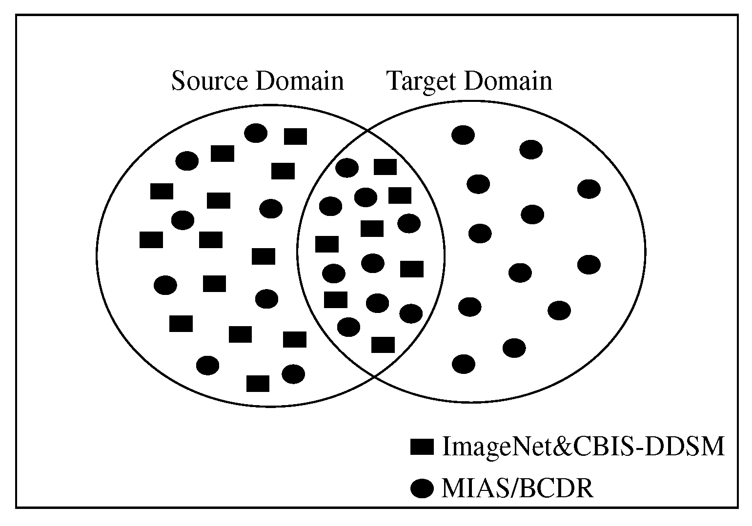Unlike TrAdaBoost [27] that filters out instances which are dissimilar to the target domain in source domains, the proposed DSTL adds new instances to the source domain ${\mathcal{D}}_s$ that are similar to the ${\mathcal{D}}_t$ to update the weights of the parameters in the pre-trained models in the ${\mathcal{D}}_s$ and form a distribution similar to the target domain. 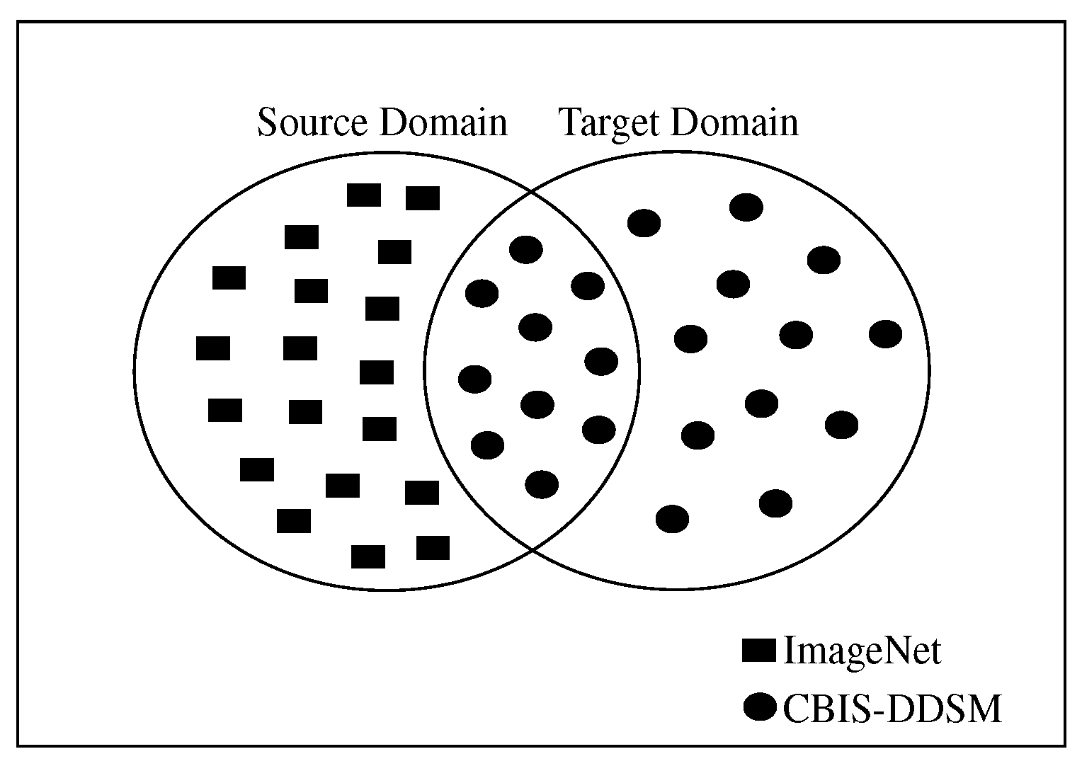Figure 3 and Figure 4 show a sketch of the instances transferring in SSTL and DSTL respectively.

Definition 1 (Standard Transfer Learning). 

Given a source domain ${\mathcal{D}}_s$ and learning task ${\mathcal{T}}_s$, a target domain ${\mathcal{D}}_t$ and learning task ${\mathcal{T}}_t$, transfer learning aims to help improve the learning of the target predictive function $f(.)$ in ${\mathcal{D}}_t$ using the knowledge in ${\mathcal{D}}_s$ and ${\mathcal{T}}_s$, where ${\mathcal{D}}_s\ne {\mathcal{D}}_t$ and/or ${\mathcal{T}}_s\ne {\mathcal{T}}_t$. ${\mathcal{D}}_s\ne {\mathcal{D}}_t$ implies that either ${\mathcal{X}}_s\ne {\mathcal{X}}_t$ or $P_s\left(X\right)\ne P_t\left(X\right)$. ${\mathcal{T}}_s\ne {\mathcal{T}}_t$ implies that either ${\mathcal{Y}}_s\ne {\mathcal{Y}}_t$ or $P\left(Y_s\right|X_s)\ne P\left(Y_t\right|X_t)$.

Definition 2 (DSTL). 

Given a source domain ${\mathcal{D}}_s$ and learning task ${\mathcal{T}}_s$, a target domain ${\mathcal{D}}_t$ and learning task ${\mathcal{T}}_t$, transfer learning aims to help improve the learning of the target predictive function $f(.)$ in ${\mathcal{D}}_t$ using the knowledge in ${\mathcal{D}}_s$ and ${\mathcal{T}}_s$, where ${\mathcal{D}}_s\simeq {\mathcal{D}}_t$ and ${\mathcal{T}}_s\simeq {\mathcal{T}}_t$. ${\mathcal{D}}_s\simeq {\mathcal{D}}_t$ implies that ${\mathcal{X}}_s\simeq {\mathcal{X}}_t$ and $P_s\left(X\right)\simeq P_t\left(X\right)$. ${\mathcal{T}}_s\simeq {\mathcal{T}}_t$ implies that ${\mathcal{Y}}_s\simeq {\mathcal{Y}}_t$ and $P\left(Y_s\right|X_s)\simeq P\left(Y_t\right|X_t)$.

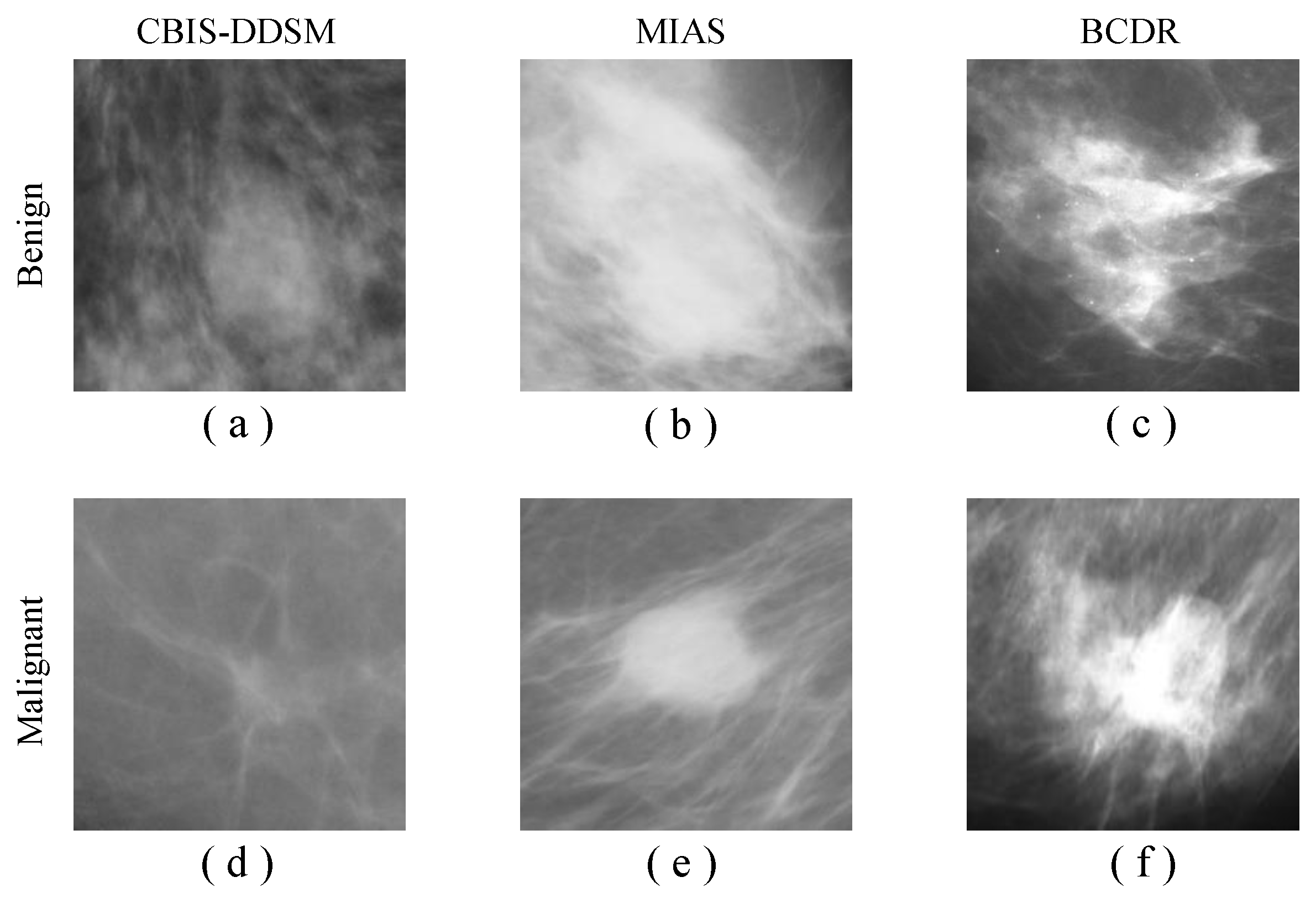
In our context, the learning task is image classification (Benign or Malignant), and each pixel or weight is taken as a feature, hence $\mathcal{X}$ is the space of all pixel vectors, $x_i$ is the ith pixel vector corresponding to some images and X is a specific learning sample. Additionally, $\mathcal{Y}$ is the set of all labels, which is Benign, Malignant for the classification task, and $y_i$ is “Benign” or “Malignant”. In our context, ${\mathcal{D}}_s$ can be a set of weights vectors together with their associated Benign or Malignant class labels. Based on the above DSTL definition, a domain is a pair $\mathcal{D}=\{\mathcal{X},P(X\left)\right\}$, hence, the condition ${\mathcal{D}}_s\simeq {\mathcal{D}}_t$ implies that ${\mathcal{X}}_s\simeq {\mathcal{X}}_t$ and $P_s\left(X\right)\simeq P_t\left(X\right)$. This indicates that the images features or their marginal distributions in both ${\mathcal{D}}_s$ and ${\mathcal{D}}_t$ are related. Similarly, a task is defined as a pair $\mathcal{T}=\{\mathcal{Y},P(Y\left|X\right)\}$, hence, the condition ${\mathcal{T}}_s\simeq {\mathcal{T}}_t$ implies that ${\mathcal{Y}}_s\simeq {\mathcal{Y}}_t$ and $P\left(Y_s\right|X_s)\simeq P\left(Y_t\right|X_t)$. When the ${\mathcal{D}}_t$ = ${\mathcal{D}}_s$ and ${\mathcal{T}}_t$ = ${\mathcal{T}}_s$, the learning task becomes a traditional machine learning task. Moreover, when ${\mathcal{D}}_t\ne {\mathcal{D}}_s$, then either (1) ${\mathcal{X}}_t\ne {\mathcal{X}}_s$ or (2) ${\mathcal{X}}_t={\mathcal{X}}_s$ but $P\left(X_s\right)\ne P\left(X_t\right)$, where $X_{s_i}\in {\mathcal{X}}_s$ and $X_{t_i}\in {\mathcal{X}}_t$. In our case, situation (1) refers to when one set of images is medical images and the other set is natural images. Situation (2) can correspond to when the ${\mathcal{D}}_s$ and the ${\mathcal{D}}_t$ images come from different patients or sources. Eventually, since medical images share many features in common compared to natural images, DSTL technique creates an implicit relationship between ${\mathcal{D}}_s$ and ${\mathcal{D}}_t$ and extracts better feature maps than the pr-trained models that have been only trained on natural images.

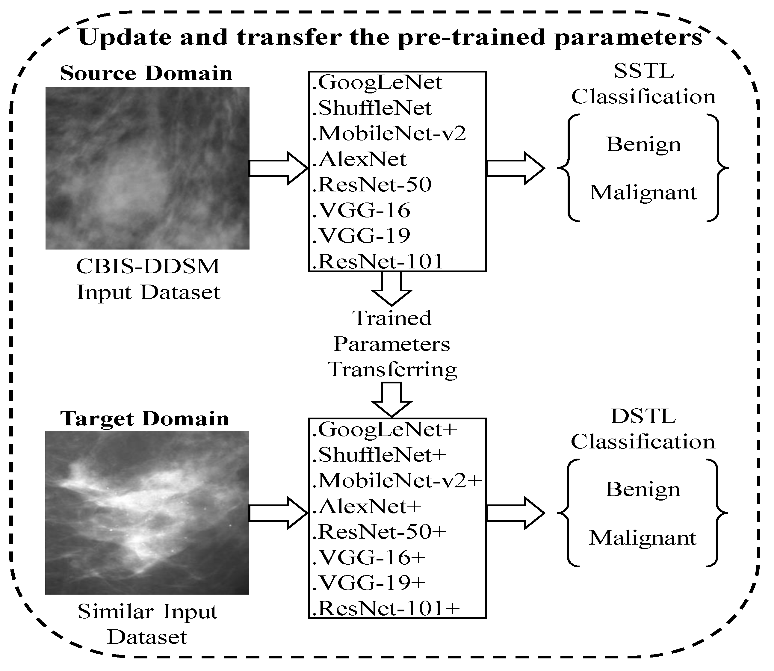
DSTL can be considered as a new strategy for adjusting the weights of the pre-trained models by mapping the instances from ${\mathcal{D}}_s$ and ${\mathcal{D}}_t$ to a new domain space. The new space will contain instances from ${\mathcal{D}}_s$ and ${\mathcal{D}}_t$, making it domain invariant. In this research, various pr-trained models were fine-tuned on 98,967 of the augmented CBIS-DDSM dataset, and saved as the name of the original pre-trained network followed by the symbol (+) to distinguish them from the original pre-trained networks that were only trained on ImageNet dataset. Next, the updated pre-trained models (+) were fine-tuned for the second time on the augmented images of the target datasets of MIAS and BCDR. Figure 5 illustrates the process of DSTL. All the pre-trained networks that have been used in this research share three common layers namely input layer, FC layer, and classification layer. By fine-tuning these 3 layers using the CBIS-DDSM dataset first, we can update all the learnable parameters, and then augment them on the target datasets of MIAS and BCDR datasets. 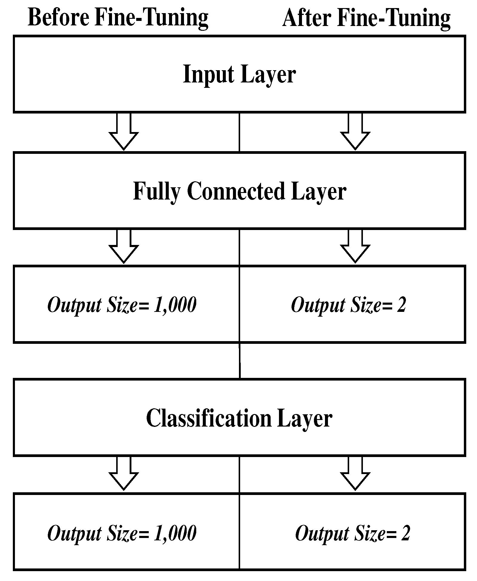Figure 6 shows the fine-tuned layers where the input layer size is kept the same as the original one $224\times 224$ except for Alexnet where the input size was set to $227\times 227$. FC and classification layers were fine-tuned in every pre-trained model. Every pre-trained model has been fine-tuned by replacing the output size parameter of FC and classification layers from classifying images of 1,000 object categories to 2 classes of benign and malignant. The classification layer computes the cross entropy loss with mutually exclusive classes. The classification layer takes the output from the Softmax layer and allocates each input to one of the K mutually exclusive classes using the cross entropy function. In Figure 6, we only mention the layers which have been fine-tuned respectively.

It is worth mentioning that although the CBIS-DDSM, MIAS, and BCDR datasets are similar, they come from different sources. Thus, these medical datasets have not been combined as a single dataset for this research experiment. This will shed light on the use of the DSTL technique in various medical image classification tasks such as liver cancer, lung cancer, kidney cancer, and other types of cancers, where the collection of high-quality annotated images is very expensive. However, due to the availability of the breast cancer datasets, the DSTL has been applied to the breast cancer classification.

3. Execution Environment

All the experiments were performed using a PC with Intel^®Core^TM i5-8400, CPU @ 2.80GHz x 6, and 23 GB of RAM. NVIDIA^®TITAN Xp GPU with 12 GB of memory. MATLAB R2019b with CUDA V10.2 and cuDNN 7.6.5. The operating system is 64-bit Ubuntu 18.04.3.

4. Results

The most common performance evaluation metrics in the field of computer vision and image process were used for evaluating the performance of the pre-trained models with SSTL and DSTL for classifying between benign and malignant breast X-ray images. The evaluation methods include Sensitivity, Specificity, Classification Accuracy, and Receiver Operating Characteristic curve [28,29,30,31]. Finally, the performance analysis of different pre-trained network is demonstrated, including the training time, epoch number, and iteration number.

4.1. Sensitivity

It is also called the true positive (TP) rate. TP corresponds to Malignant cases in this research. It calculates the number of true positive predictions over the number of actual positive plus false negative (FN) cases, defined as:

$$Sensitivity=\frac{TP}{TP+FN}$$

(1)

4.2. Specificity

It can be called the true negative (TN) rate. In this paper, TN corresponds to Benign cases. It computes the proportion of actual negative cases that are predicted as negative cases. The specificity formula is defined as:

$$Specificity=\frac{TN}{TN+FP}$$

(2)

4.3. Accuracy

Accuracy or overall accuracy represents the number of correctly predicted cases over the all cases. It can be formulated as:

$$Accuracy=\frac{TN+TP}{TN+TP+FP+FN}$$

(3)

4.4. Receiver Operating Characteristic (ROC)

In this paper, the ROC curve is used to evaluate the performance quality of the pre-trained models and present the Area Under the Curve (AUC) by applying threshold values across the interval [0,1]. For each threshold, two values are calculated, the probability of detection power $P_D$ or the TP ratio and the probability of false alarm or the false positive (FP) ratio. Figure 7, Figure 8, Figure 9 and Figure 10 show the ROC curve which was used to plot TP versus FP with the threshold as a parameter for AlexNet, VGG-16, VGG-19, GoogLeNet, ResNet-50, ResNet-101, MobileNet-v2, and ShuffleNet on MIAS, and BCDR datasets, respectively.

Table 7. Comparison of various pre-trained models performance using the CBIS-DDSM dataset.

Dataset	Model	Val. Acc.	Testing Acc.	Specificity	Sensitivity	AUC
	AlexNet	90.18%	81.92%	86.65%	76.11%	89.24%
	ShuffleNet	93.85%	89.28%	92.51%	85.30%	95.46%
	MobileNet-v2	94.50%	92.03%	93.39%	90.35%	96.20%
	GoogleNet	96.56%	93.68%	96.26%	90.50%	97.47%
CBIS-DDSM	ResNet-50	96.97%	93.20%	95.26%	90.65%	96.59%
	ResNet-101	97.09%	93.47%	95.88%	90.50%	97.57%
	VGG-16	96.20%	92.58%	93.76%	91.18%	97.11%
	VGG-19	95.12%	90.93%	93.02%	88.36%	96.65%

demonstrates the results summary of the pre-trained models using single-shot transfer learning using the CBIS-DDSM dataset. It can be noted from Table 7 that most of the pre-trained models have produced resealable results due to the large number of training samples they were trained on.

Table 8. The comparison of various pre-trained models with SSTL and DSTL on MIAS and BCDR datasets.

Dataset & Technique	Model	Validation Acc.	Testing Acc.	Specificity	Sensitivity	AUC
	AlexNet	56.07%	88.60%	92.06%	84.31%	96.14%
	ShuffleNet	68.73%	92.98%	93.65%	92.15%	96.64%
	MobileNet-v2	64.60%	92.11%	93.65%	90.19%	96.20%
MIAS	GoogLeNet	60.21%	88.60%	95.24%	80.39%	98.41%
(With SSTL)	ResNet-50	72.35%	93.86%	95.24%	92.15%	98.41%
	ResNet-101	70.80%	91.23%	95.24%	86.27%	97.60%
	VGG-16	66.15%	92.11%	96.83%	86.27%	98.23%
	VGG-19	57.88%	90.35%	90.48%	90.19%	97.45%
	AlexNet+	61.50%	92.11%	95.24%	88.24%	96.92%
	ShuffleNet+	80.88%	96.49%	96.82%	96.07%	99.44%
	MobileNet-v2+	83.46%	98.25%	98.41%	98.03%	99.53%
MIAS	GoogLeNet+	86.30%	96.49%	98.41%	94.11%	99.69%
(With DSTL)	ResNet-50+	82.43%	95.61%	96.82 %	94.11%	99.25%
	ResNet-101+	87.08%	97.37%	98.41%	96.07%	99.60%
	VGG-16+	77.00%	93.86%	96.82%	90.19%	99.04%
	VGG-19+	76.23%	93.86%	95.24%	92.16%	99.28%
	AlexNet	65.20%	73.38%	77.27%	69.46%	80.64%
	ShuffleNet	70.86%	81.75%	75.75%	87.78%	88.57%
	MobileNet-v2	69.60%	82.13%	80.30%	83.96%	88.71%
BCDR	GoogLeNet	74.00%	83.65%	83.33%	83.96%	91.59%
(With SSTL)	ResNet-50	73.38%	77.95%	70.45%	85.49%	85.94%
	ResNet-101	77.78%	81.37%	77.27%	85.49%	89.90%
	VGG-16	73.17%	79.09%	77.27%	80.92%	89.14%
	VGG-19	81.97%	84.41%	82.57%	86.25%	91.99%
	AlexNet+	77.36%	82.13%	83.33%	80.91%	93.20%
	ShuffleNet+	81.97%	87.83%	86.36%	89.31%	94.74%
	MobileNet-v2+	82.39%	86.31%	80.30%	92.36%	91.51%
BCDR	GoogLeNet+	87.84%	88.21%	86.36%	90.07%	95.65%
(With DSTL)	ResNet-50+	83.65%	87.07%	84.09%	90.07%	93.92%
	ResNet-101+	82.81%	87.07%	81.06%	93.13%	94.29%
	VGG-16+	81.76%	87.97%	90.91%	87.02%	94.52%
	VGG-19+	86.79%	89.11%	89.39%	90.84%	94.57%

shows the comparison summary of the pre-trained models with SSTL and DSTL technique.

Table 9. The performance analysis of different pre-trained networks with SSTL and DSTL on MIAS and BCDR datasets.

Dataset & Technique	Model	Training-Time	Epoch	Iteration
	AlexNet	04 min 22 s	48	1824
	ShuffleNet	17 min 51 s	38	1444
	MobileNet-v2	12 min 17 s	20	760
MIAS	GoogLeNet	08 min 50 s	29	1102
(With SSTL)	ResNet-50	11 min 30 s	18	684
	ResNet-101	37 min 17 s	25	950
	VGG-16	09 min 55 s	21	798
	VGG-19	25 min 13 s	46	1748
	AlexNet+	02 min 43 s	21	798
	ShuffleNet+	11 min 49 s	28	1064
	MobileNet-v2+	11 min 35 s	19	722
MIAS	GoogLeNet+	08 min 08 s	25	950
(With DSTL)	ResNet-50+	09 min 54 s	16	608
	ResNet-101+	31 min 23 s	21	798
	VGG-16+	08 min 22 s	18	684
	VGG-19+	08 min 48 s	15	570
	AlexNet	02 min 45 s	42	1974
	ShuffleNet	10 min 30 s	30	1410
	MobileNet-v2	09 min 51 s	23	1081
BCDR	GoogLeNet	05 min 51 s	28	1316
(With SSTL)	ResNet-50	21 min 37 s	42	1974
	ResNet-101	13 min 38 s	14	658
	VGG-16	11 min 56 s	21	987
	VGG-19	28 min 11 s	43	2021
	AlexNet+	02 min 40 s	41	1927
	ShuffleNet+	05 min 02 s	16	752
	MobileNet-v2+	07 min 13 s	17	799
BCDR	GoogLeNet+	03 min 32 s	17	799
(With DSTL)	ResNet-50+	15 min 13 s	30	1410
	ResNet-101+	11 min 04 s	11	517
	VGG-16+	09 min 30 s	15	705
	VGG-19+	08 min 27 s	13	611

illustrates the comparison summary of the performance evaluation of different pre-trained models in terms of the training time, number of epochs, and number of iterations. As can be seen from Table 8 and Table 9, the DSTL technique has improved the accuracy and performance of the pre-trained networks significantly. In this research, instead of reinventing the wheel, the existing pre-trained models have been used to evaluate the method of transfer learning from ImageNet (SSTL) against our proposed technique (DSTL). We did not consider training from random initialization as the case in [32]. By observing the results in Table 8, it is obvious that DSTL can enhance the performance of the lightweight and non-lightweight models alike and provide faster convergence as shown in Table 9. However, training from random initialization can be analyzed in the future.

In Table 9, the number of iterations and epochs is different for each model because we use the validation accuracy monitoring algorithm which helps with reducing the number of iterations and epochs by keeping track of the best validation accuracy and the number of validations, hence, when there has not been any improvement of the validation accuracy (validation lag), an early stop mode of the training process will be triggered. For example, if the validation accuracy is not improving after 10 iterations, the training process will stop automatically.

5. Conclusions

In this research, an effective transfer learning technique called double-shot transfer learning (DSTL) has been introduced to improve the overall accuracy and performance of various pre-trained models, especially in the field of medical image analysis. Simple and effective image augmentation techniques were also used to overcome the lack of breast X-ray images, improve invariance, and reduce overfitting by generating new training samples based on the existing breast X-ray images manipulations. The most common image display functions performed by doctors and radiologists during the diagnostic image viewing have been considered as the augmentation methods for this research. The proposed technique will overcome the lack of available training samples issues, improve the pre-trained models accuracy and performance, and will provide a valuable solution to the difference between the source and target domain problem in transfer learning.

References

1. Alkhaleefah, M.; Wu, C.C. A Hybrid CNN and RBF-Based SVM Approach for Breast Cancer Classification in Mammograms. In Proceedings of the IEEE International Conference on Systems, Man, and Cybernetics (SMC), Miyazaki, Japan, 7–10 October 2018; pp. 894–899. [Google Scholar]
2. Greenspan, H.; Van Ginneken, B.; Summers, R.M. Guest editorial deep learning in medical imaging: Overview and future promise of an exciting new technique. IEEE Trans. Med. Imaging 2016, 35, 1153–1159. [Google Scholar] [CrossRef]
3. Ching, T.; Himmelstein, D.S.; Beaulieu-Jones, B.K.; Kalinin, A.A.; Do, B.T.; Way, G.P.; Ferrero, E.; Agapow, P.M.; Zietz, M.; Hoffman, M.M.; et al. Opportunities and obstacles for deep learning in biology and medicine. J. R. Soc. Interface 2018, 15, 20170387. [Google Scholar] [CrossRef] [PubMed] [Green Version]
4. Lévy, D.; Jain, A. Breast mass classification from mammograms using deep convolutional neural networks. arXiv 2016, arXiv:1612.00542. [Google Scholar]
5. Hussain, Z.; Gimenez, F.; Yi, D.; Rubin, D. Differential data augmentation techniques for medical imaging classification tasks. In Proceedings of the AMIA Annual Symposium, Washington, DC, USA, 4–8 November 2017; p. 979. [Google Scholar]
6. Chen, Y.; Zhang, Q.; Wu, Y.; Liu, B.; Wang, M.; Lin, Y. Fine-Tuning ResNet for Breast Cancer Classification from Mammography. In Proceedings of the International Conference on Healthcare Science and Engineering, Guilin, China, 1–3 June 2018; pp. 83–96. [Google Scholar]
7. Falconí, L.G.; Pérez, M.; Aguilar, W.G. Transfer Learning in Breast Mammogram Abnormalities Classification With Mobilenet and Nasnet. In Proceedings of the International Conference on Systems, Signals and Image Processing (IWSSIP), Osijek, Croatia, 5–7 June 2019; pp. 109–114. [Google Scholar]
8. Huynh, B.Q.; Li, H.; Giger, M.L. Digital mammographic tumor classification using transfer learning from deep convolutional neural networks. J. Med. Imaging 2016, 3, 034501. [Google Scholar] [CrossRef] [PubMed]
9. Vesal, S.; Ravikumar, N.; Davari, A.; Ellmann, S.; Maier, A. Classification of breast cancer histology images using transfer learning. In Proceedings of the International Conference Image Analysis and Recognition, Póvoa de Varzim, Portugal, 27–29 June 2018; pp. 812–819. [Google Scholar]
10. Shan, H.; Wang, G.; Kalra, M.K.; de Souza, R.; Zhang, J. Enhancing transferability of features from pretrained deep neural networks for lung nodule classification. In Proceedings of the 2017 International Conference on Fully Three-Dimensional Image Reconstruction in Radiology and Nuclear Medicine, Xi’an, China, 18–23 June 2017; pp. 65–68. [Google Scholar]
11. Krizhevsky, A.; Sutskever, I.; Hinton, G.E. Imagenet classificationwith deep convolutional neural networks. In Proceedings of the 26th Conference on Neural Information Processing Systems, Lake Tahoe, NV, USA, 3–6 December 2012; pp. 1097–1105. [Google Scholar]
12. Simonyan, K.; Zisserman, A. Very deep convolutional networks for large-scale image recognition. arXiv 2014, arXiv:1409.1556. [Google Scholar]
13. Szegedy, C.; Liu, W.; Jia, Y.; Sermanet, P.; Reed, S.; Anguelov, D.; Erhan, D.; Vanhoucke, V.; Rabinovich, A. Going deeper with convolutions. In Proceedings of the 28th IEEE conference on computer vision and pattern recognition, Boston, MA, USA, 7–12 June 2015; pp. 1–9. [Google Scholar]
14. He, K.; Zhang, X.; Ren, S.; Sun, J. Deep residual learning for image recognition. In Proceedings of the IEEE Conference on Computer Vision and Pattern Recognition, Las Vegas, NV, USA, 27–30 June 2016; pp. 770–778. [Google Scholar]
15. Sandler, M.; Howard, A.; Zhu, M.; Zhmoginov, A.; Chen, L.C. Mobilenetv2: Inverted residuals and linear bottlenecks. In Proceedings of the IEEE Conference on Computer Vision and Pattern Recognition, Salt Lake City, UT, USA, 18–23 June 2018; pp. 4510–4520. [Google Scholar]
16. Zhang, X.; Zhou, X.; Lin, M.; Sun, J. Shufflenet: An extremely efficient convolutional neural network for mobile devices. In Proceedings of the IEEE Conference on Computer Vision and Pattern Recognition, Salt Lake City, UT, USA, 18–23 June 2018; pp. 6848–6856. [Google Scholar]
17. Heath, M.; Bowyer, K.; Kopans, D.; Moore, R.; Kegelmeyer, W.P. The digital database for screening mammography. In Proceedings of the 5th International Workshop on Digital Mammography, Toronto, ON, Canada, 11–14 June 2000; pp. 212–218. [Google Scholar]
18. Lee, R.S.; Gimenez, F.; Hoogi, A.; Miyake, K.K.; Gorovoy, M.; Rubin, D. A curated mammography data set for use in computer-aided detection and diagnosis research. Sci. Data 2017, 4, 170177. [Google Scholar] [CrossRef] [PubMed]
19. The Mini-MIAS Database of Mammograms. Available online: http://peipa.essex.ac.uk/info/mias.html (accessed on 1 January 2020).
20. Suckling, J. The Mammographic Image Analysis Society Digital Mammogram Database. In 2nd International Workshop on Digital Mammography; Elsevier Science: Amsterdam, The Netherlands, 1994; pp. 375–378. [Google Scholar]
21. Lopez, M.G.; Posada, N.; Moura, D.C.; Pollán, R.R.; Valiente, J.M.F.; Ortega, C.S.; Solar, M.; Diaz-Herrero, G.; Ramos, I.M.A.P.; Loureiro, J.; et al. BCDR: A breast cancer digital repository. In Proceedings of the 15th International Conference on Experimental Mechanics, Porto, Portugal, 22–27 July 2012; pp. 1–5. [Google Scholar]
22. Srivastava, N.; Hinton, G.; Krizhevsky, A.; Sutskever, I.; Salakhutdinov, R. Dropout: A simple way to prevent neural networks from overfitting. J. Mach. Learn. Res. 2014, 15, 1929–1958. [Google Scholar]
23. Chen, Y.; Jiang, H.; Li, C.; Jia, X.; Ghamisi, P. Deep feature extraction and classification of hyperspectral images based on convolutional neural networks. IEEE Trans. Geosci. Remote Sens. 2016, 54, 6232–6251. [Google Scholar] [CrossRef] [Green Version]
24. Alkhaleefah, M.; Chittem, P.K.; Achhannagari, V.P.; Ma, S.C.; Chang, Y.L. The Influence of Image Augmentation on Breast Lesion Classification Using Transfer Learning. In Proceedings of the 2020 International Conference on Artificial Intelligence and Signal Processing (AISP), Amaravati, India, 10–12 January 2020; pp. 1–5. [Google Scholar]
25. Zhuang, F.; Qi, Z.; Duan, K.; Xi, D.; Zhu, Y.; Zhu, H.; Xiong, H.; He, Q. A Comprehensive Survey on Transfer Learning. Available online: https://arxiv.org/pdf/1911.02685.pdf (accessed on 4 January 2020).
26. Pan, S.J.; Yang, Q. A survey on transfer learning. IEEE Trans. Knowl. Data Eng. 2009, 10, 1345–1359. [Google Scholar] [CrossRef]
27. Wenyuan, D.; Yang, Q.; Xue, G.; Yu, Y. Boosting for transfer learning. In Proceedings of the 24th International Conference on Machine Learning, Corvallis, OR, USA, 20–24 June 2007; pp. 193–200. [Google Scholar]
28. Baldi, P.; Brunak, S.; Chauvin, Y.; Andersen, C.A.; Nielsen, H. Assessing the accuracy of prediction algorithms for classification: An overview. Bioinformatics 2000, 16, 412–424. [Google Scholar] [CrossRef] [PubMed] [Green Version]
29. Carroll, H.D.; Kann, M.G.; Sheetlin, S.L.; Spouge, J.L. Threshold Average Precision (TAP-k): A measure of retrieval designed for bio-informatics. Bioinformatics 2010, 26, 1708–1713. [Google Scholar] [CrossRef] [PubMed] [Green Version]
30. Fawcett, T. An introduction to roc analysis. Pattern Recognit. Lett. 2006, 27, 861–874. [Google Scholar] [CrossRef]
31. Felzenszwalb, P.F.; Girshick, R.B.; McAllester, D.; Ramanan, D. Object detection with discriminatively trained part-based models. IEEE Trans. Pattern Anal. Mach. Intell. 2010, 32, 1627–1645. [Google Scholar] [CrossRef] [PubMed] [Green Version]
32. Raghu, M.; Zhang, C.; Kleinberg, J.; Bengio, S. Transfusion: Understanding transfer learning for medical imaging. In Proceedings of the Advances in Neural Information Processing Systems, Vancouver, BC, Canada, 8–14 December 2019; pp. 3342–3352. [Google Scholar]
Figure 1. Examples of noisy and corrupted images. (a,b) contain some black arrow marks made by doctors or radiologists indicating the location of the lesion. (c) is a result of insufficient illumination or incorrect device adjustment.
Applsci 10 03999 g001
Figure 2. Datasets examples. Benign cases are shown in (ac). Malignant cases are shown in (df). (a,d) represent samples from the curated breast imaging subset of digital database screening mammography (CBIS-DDSM) dataset, (b,e) represent samples from the mammographic image analysis society (MIAS) dataset, and (c,f) represent samples from the breast cancer digital repository (BCDR) dataset.
Applsci 10 03999 g002
Figure 3. Sketching the instances transferring in single-shot transfer learning (SSTL), where some instances from similar D t (CBIS-DDSM) are included in the D s (ImageNet) to update the weights in the pre-trained models.
Applsci 10 03999 g003
Figure 4. Sketching the instances transferring in double-shot transfer learning (DSTL), where some instances from the D t (MIAS or BCDR) are included in the D s (ImageNet and CBIS-DDSM). Note that SSTL has made the CBIS-DDSM instances part of the D s .
Applsci 10 03999 g004
Figure 5. The process of DSTL, where various pre-trained models were first fine-tuned on a large number of the augmented CBIS-DDSM dataset to update their weights and biases parameters. Second, the updated pre-trained models were fine-tuned on a new and similar dataset to classify between benign and malignant.
Applsci 10 03999 g005
Figure 6. The three fine-tuned layers for every pre-trained model.
Applsci 10 03999 g006
Figure 7. The receiver operating characteristic (ROC) curve of various pre-trained models with SSTL for breast cancer classification using the MIAS dataset.
Applsci 10 03999 g007
Figure 8. The ROC curve of various pre-trained models with DSTL for breast cancer classification using the MIAS dataset, where the AUC of each pre-trained model has been improved.
Applsci 10 03999 g008
Figure 9. The ROC curve of various pre-trained models with SSTL for breast cancer classification using the BCDR dataset.
Applsci 10 03999 g009
Figure 10. The ROC curve of various pre-trained models with DSTL for breast cancer classification using the BCDR dataset.
Applsci 10 03999 g010