Nighttime Vehicle Detection and Tracking with Occlusion Handling by Pairing Headlights and Taillights

Abstract

In recent years, vision-based vehicle detection has received considerable attention in the literature. Depending on the ambient illuminance, vehicle detection methods are classified as daytime and nighttime detection methods. In this paper, we propose a nighttime vehicle detection and tracking method with occlusion handling based on vehicle lights. First, bright blobs that may be vehicle lights are segmented in the captured image. Then, a machine learning-based method is proposed to classify whether the bright blobs are headlights, taillights, or other illuminant objects. Subsequently, the detected vehicle lights are tracked to further facilitate the determination of the vehicle position. As one vehicle is indicated by one or two light pairs, a light pairing process using spatiotemporal features is applied to pair vehicle lights. Finally, vehicle tracking with occlusion handling is applied to refine incorrect detections under various traffic situations. Experiments on two-lane and four-lane urban roads are conducted, and a quantitative evaluation of the results shows the effectiveness of the proposed method.

1. Introduction

With the aim of making every facet of citizens’ lives easy, various technologies and solutions have been studied for intelligent transportation system (ITS) applications in recent years. The aim of an ITS is to provide users with traffic information that enables them to make safer and smarter use of transportation networks. Among many ITS technologies, vision-based vehicle detection has played a vital role in many applications, such as traffic control, traffic surveillance, and autonomous driving. Compared to other sensors such as lidar and radar [1,2,3], camera-based sensors are more preferable owing to such benefits as easy installation, low-cost maintenance, and high flexibility. Furthermore, the emergence of parallel computing, including multicore processing and graphical processing units, has allowed the pursuit of the real-time implementation of vision-based vehicle detection methods.

To detect on-road vehicles, most vehicle detection methods use vehicle appearances as the main features [4]. In the absence of details regarding vehicle appearance, detecting vehicles at nighttime is more challenging than in the daytime. In the daytime, vehicle detection is based on the color, shape, shadow, corners, and edges of vehicles [5]. On the other hand, at night, the abovementioned features are not visible because of the low contrast and luminosity of nighttime images. Under dark conditions, the most salient features are light sources, and vehicle headlights or taillights become important characteristics that can be used for identifying vehicles. Depending on the purpose of the specific system, a vehicle detection algorithm may be constructed based on headlights or taillights only or both headlights and taillights. For instance, traffic surveillance systems only detect oncoming vehicles (headlights), whereas advanced driver-assistance systems monitor preceding vehicles (taillights) or both preceding and oncoming vehicles (taillights and headlights). For nighttime vehicle detection, most existing studies execute two main steps: vehicle light identification followed by vehicle light pairing.

Various methods have been proposed to identify headlights in a captured image. Most of the methods first segment the image to find bright blobs that may be headlights. By using a fixed or adaptive threshold, a set of pixels of bright spots whose gray intensity values are higher than the threshold is retrieved. Then, to classify whether a bright blob is a headlight, rule-based or machine-learning-based methods are applied, the former of which are the most commonly used. In studies on rule-based methods [6,7], rules are constructed based on prior knowledge and statistical laws of contrast, position, size, and shape to classify headlights and other objects. The difficulty concerning rule-based methods is that the rules should be defined carefully and cover all scenarios to obtain highly accurate results. Alternatively, machine-learning-based methods have been researched recently because of their good discrimination and superior adaptability. In [8,9], a support vector machine (SVM) is applied to classify headlights and nuisance lights (reflections). Additionally, the Adaboost classifier and Haar features are combined to discriminate headlights from non-headlights in [10,11].

Unlike headlights, the dominant color of taillights is red; the redness of rear lights can be easily filtered out using color spaces. In [12], a set of thresholds for filtering red color in taillights is directly derived from automotive regulations and adapted for real-world conditions in the hue-saturation-value (HSV) color space. A Y’UV color space [13] is used to extract potential taillight candidates in an image. In [14], the mean of red intensity of vehicle taillight are used to verify whether an extracted bright blob is a vehicle.

After identifying vehicle lights, the light pairing process is conducted, since a vehicle is indicated by a pair of vehicle lights. This process can be performed by finding the similarity between two vehicle lights. The similarity of two lights is evaluated with respect to certain characteristics such as symmetry condition, size, shape, and cross-correlation [6,7,12,13]. A pairing method using optimization is proposed in [10,11], which applies motion information from the tracking and spatial context to find the correct pairs. However, this method carries high computation cost for optimizing over the entire set of candidate light pairs. Light pairing faces certain difficulties: one vehicle light may be shared by more than one light pair if two vehicles are at the same distance from the host vehicle. Moreover, the pairing process may fail when various complex situations occur on the road, such as partial vehicle occlusion, blooming effects, or turning vehicles.

To resolve the abovementioned problems, in this paper, we propose a vehicle detection and tracking system that perceives both preceding and oncoming vehicles on the road. The contributions of this work are three-fold: first, a machine-learning-based approach for detecting both headlights and taillights at night is proposed; second, a combination of motion information, correlation coefficient, and size of vehicle light is defined to pair the vehicle lights; finally, partial vehicle occlusion is solved by retrieving and analyzing tracking information from subsequent frames.

The remainder of this paper is organized as follows. Section 2 describes the entire process of the system. It contains two main blocks: vehicle detection, which detects preceding and oncoming vehicles, and vehicle tracking with occlusion handling. Then, the experimental setup and evaluation results based on a real dataset are presented in Section 3. Finally, the conclusions are drawn in Section 4.

2. Proposed Vehicle Detection and Tracking System

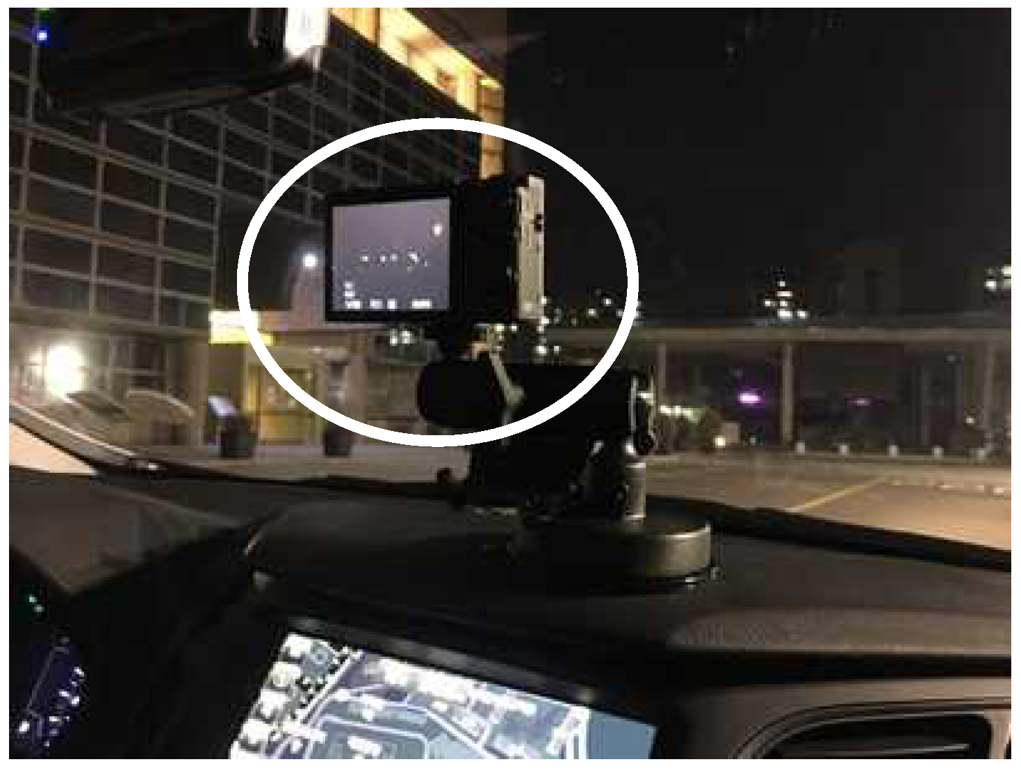
In contrast to a surveillance system which is stationary, the proposed system uses a camera mounted inside a moving vehicle. Therefore, the proposed system must cope with more complex scenarios than those faced by a traffic surveillance system. Since there is no recent studies that detect and track both oncoming and preceding vehicles in the nighttime, the proposed system is mainly derived from the studies of Chen, Y. et al. [6,7].

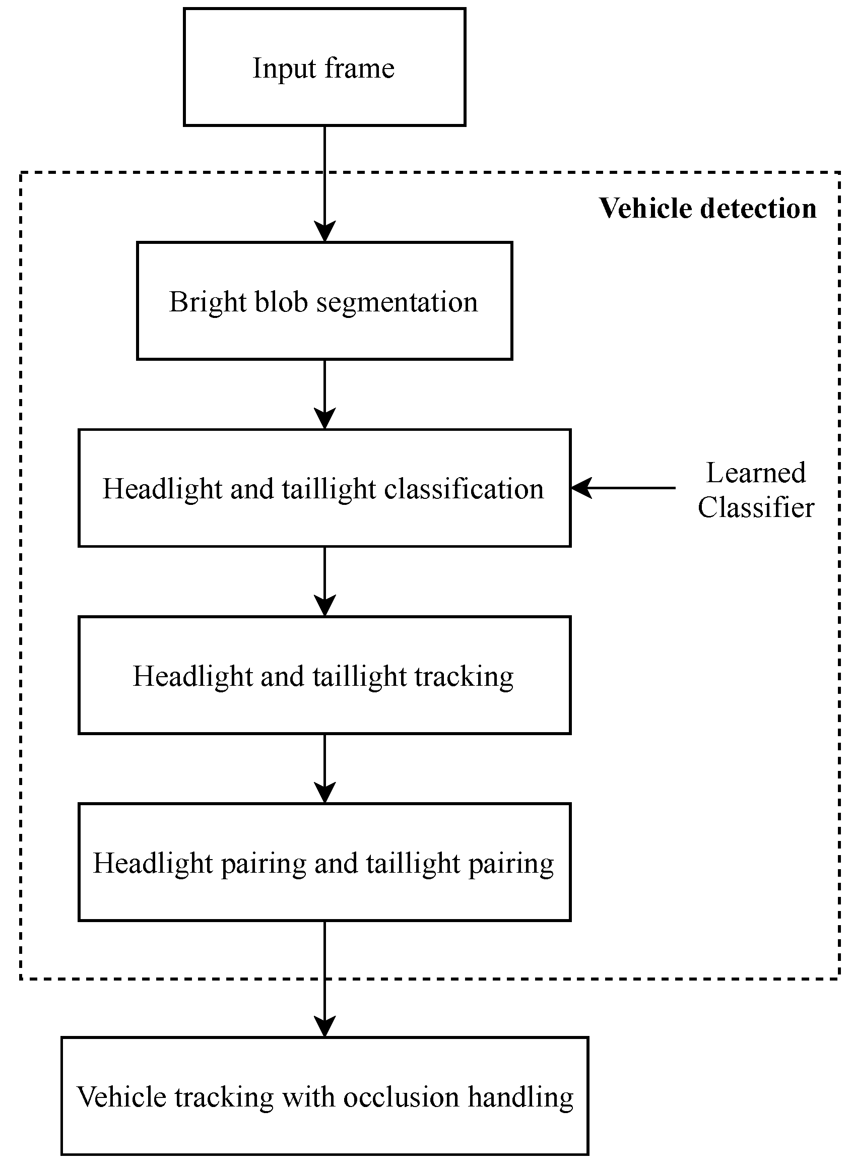
In the proposed system, five main modules are implemented sequentially, including bright blob segmentation, headlight and taillight classification, headlight and taillight tracking, headlight pairing and taillight pairing, and vehicle tracking with occlusion handling. However, before executing the online process that detects and tracks vehicles in the input image, a pre-trained offline classifier is generated to prepare for the headlight and taillight classification module. All the modules of the system are addressed in separate subsections in this paper. The overview of the proposed system is introduced in Figure 1.

2.1. Pre-Trained Offline Classifier

Based on the study of Zou [10], which outperforms other methods, in this section, a machine- learning-based method is proposed to classify both headlights and taillights in nighttime images. In the previous study, a learning headlight detector is created to discriminate headlights from non-headlights by fusing the Adaboost classifier and Haar features. However, we cannot use the previous work directly in our context, because the Adaboost classifier is a binary classifier and it has limitations in classifying multiclass data. 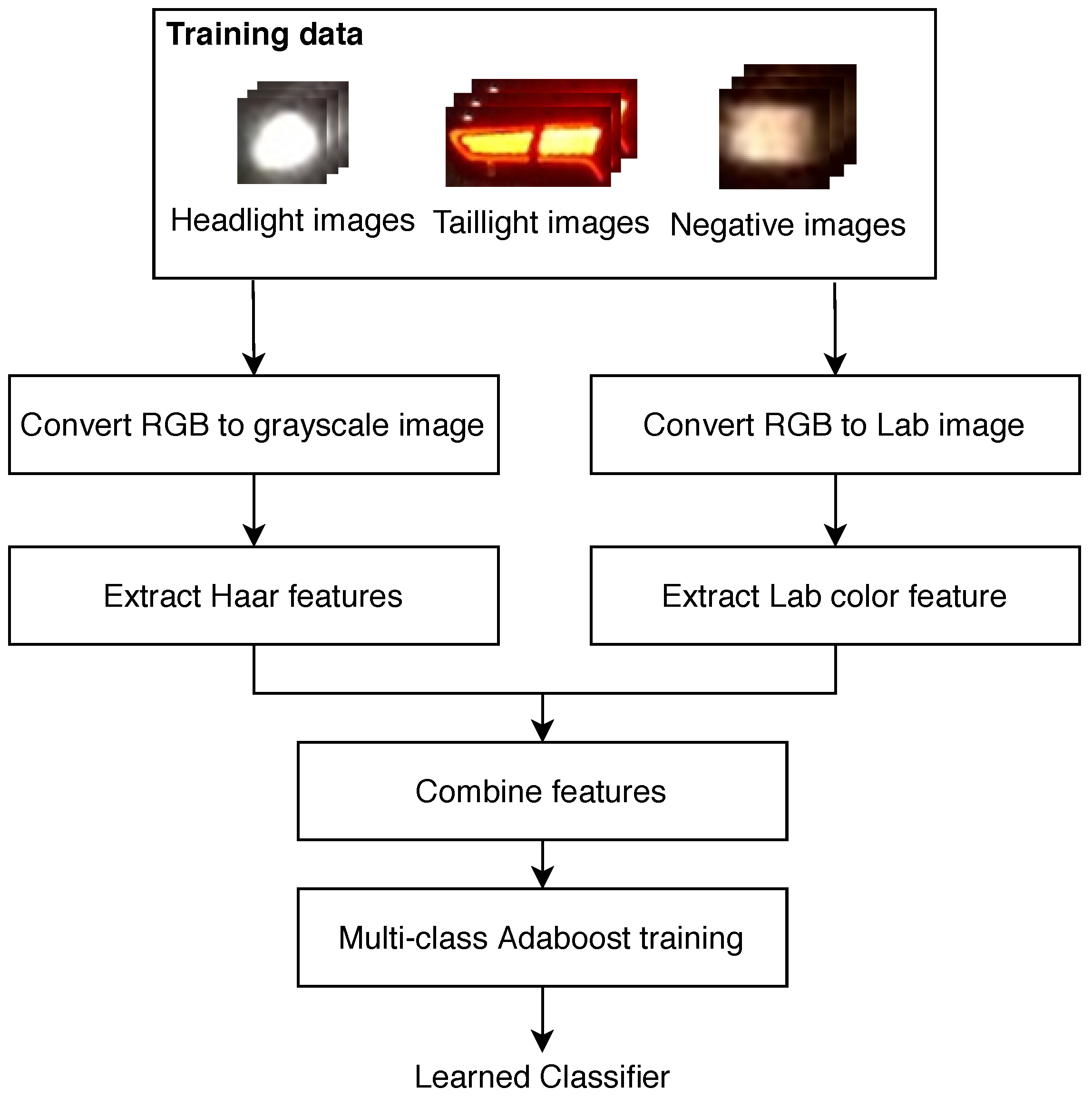Thus, we present a new method that combines the multiclass Adaboost classifier [15], Haar features, and a color feature extracted from the L*a*b* color space to discriminate head and tail lights. The proposed learning method is described as follows, according to the flowchart illustrated in Figure 2. First, a training dataset consisting of the headlight, taillight, and negative images is annotated from the captured images. Negative samples that do not contain any headlights or taillights are randomly taken. These include reflections on vehicle bodies, road surfaces, and road signs. Before extracting features, all the training images must be resized to the same dimensions, which are selected from the experiment. Next, each training image is converted from RGB to grayscale and L*a*b* color space.

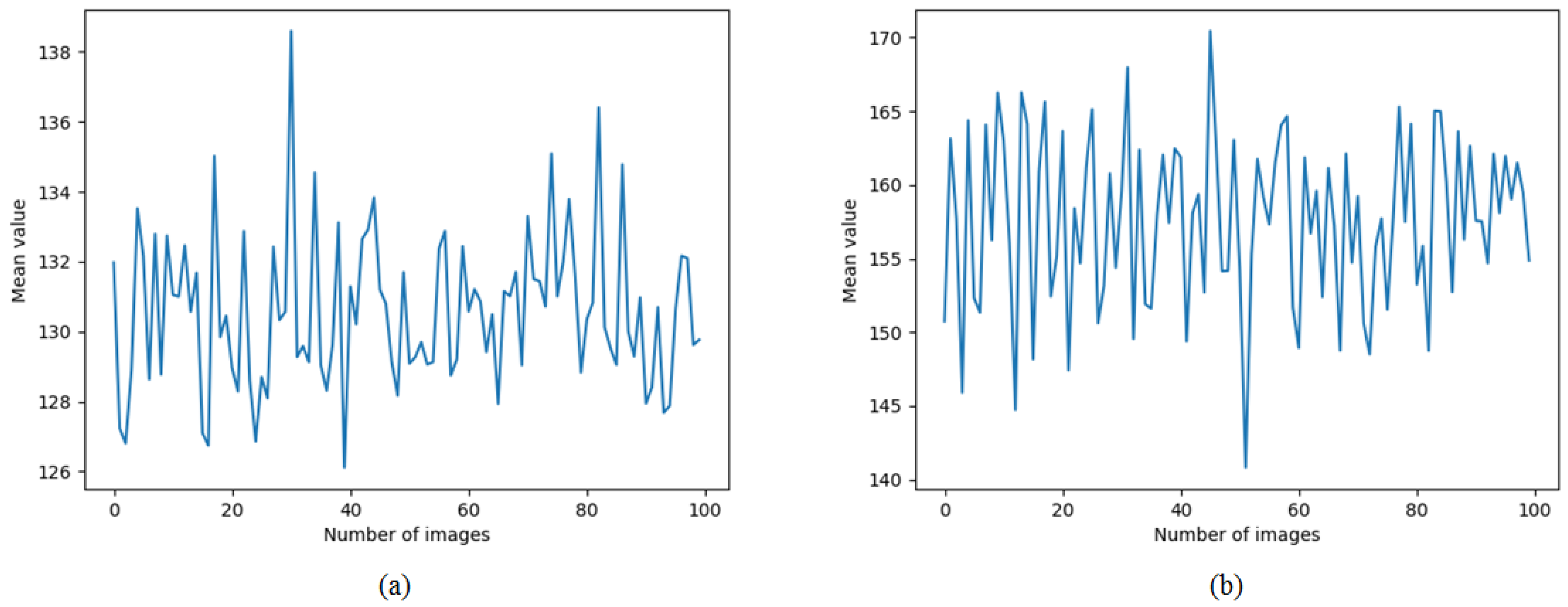
For the grayscale image, we use two-rectangle and three-rectangle features to extract Haar features. The process for extracting these features is not mentioned in this paper, as they are described in particular detail in [16]. For the L*a*b* image, only the a* channel representing the green–red color is considered. This channel is chosen statistically in the experiment and the mean value of the a* channel is calculated as the Lab color feature. The statistics of the mean values of the a* channel from 100 headlight images and 100 taillight images are depicted in Figure 3. It is clearly observable that the mean values of the a* channel of headlight images are lower than 140, whereas thoses of the a* channel of taillight images are higher than 140. Moreover, when the mean values of the a* channel from 300 headlight images and 300 taillight images are calculated, they are still at the same distribution as in the Figure 3. Therefore, the Lab color feature might be a promising feature to discriminate headlights and taillights. Finally, the combination of Haar features and the Lab color feature is input into a multiclass Adaboost classifier to train the learned classifier.

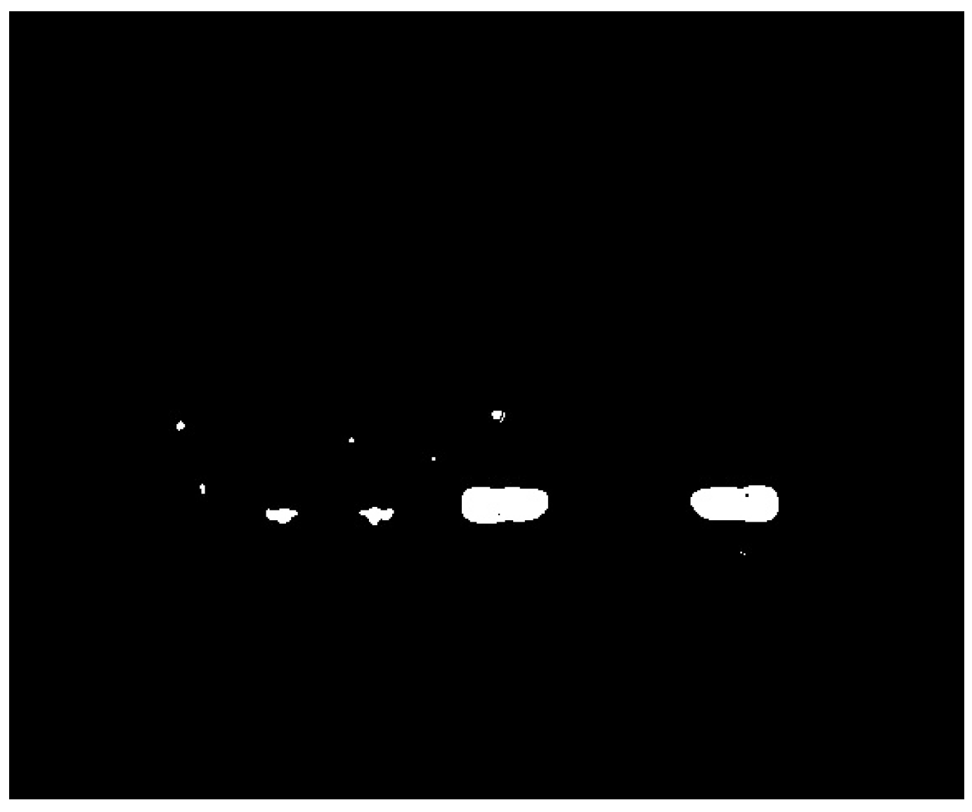
2.2. Bright Blob Segmentation

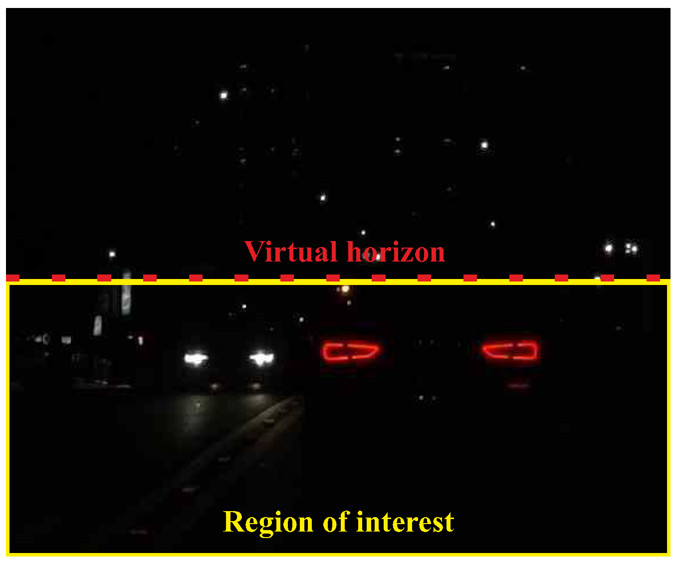
Given an RGB image retrieved from a vehicle-mounted camera, the vision-based system first extracts bright blobs that are potential vehicle lights. Because the main focus of this system is to detect and track vehicles based on vehicle lights, the nonvehicle lights such as street lamps and traffic lights should be removed from the road scene image. To filter out nuisance lights and save the computational cost, a region of interest (ROI) in which the bright blob segmentation is performed is determined. Based on the observation and the study [7], all the objects located above the virtual horizon are screened out. Thus, the ROI is the region below the virtual horizon (see Figure 4). After locating the ROI, an automatic multilevel thresholding [17] and HSV color thresholding [12] are applied to preliminarily extract potential bright blobs that might be headlights or taillights. 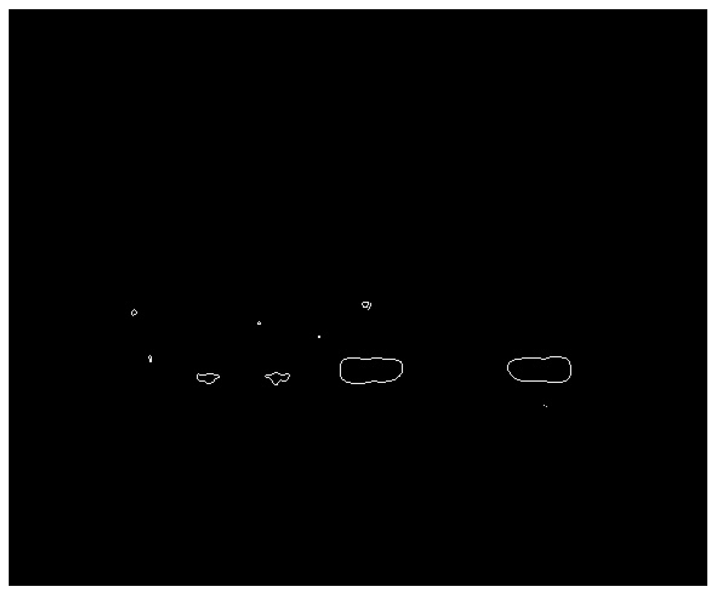As a result, a binary image containing the extracted bright blobs is created (see Figure 5). Then, the contours of extracted blobs are retrieved by using a border following algorithm [18] (see Figure 6).

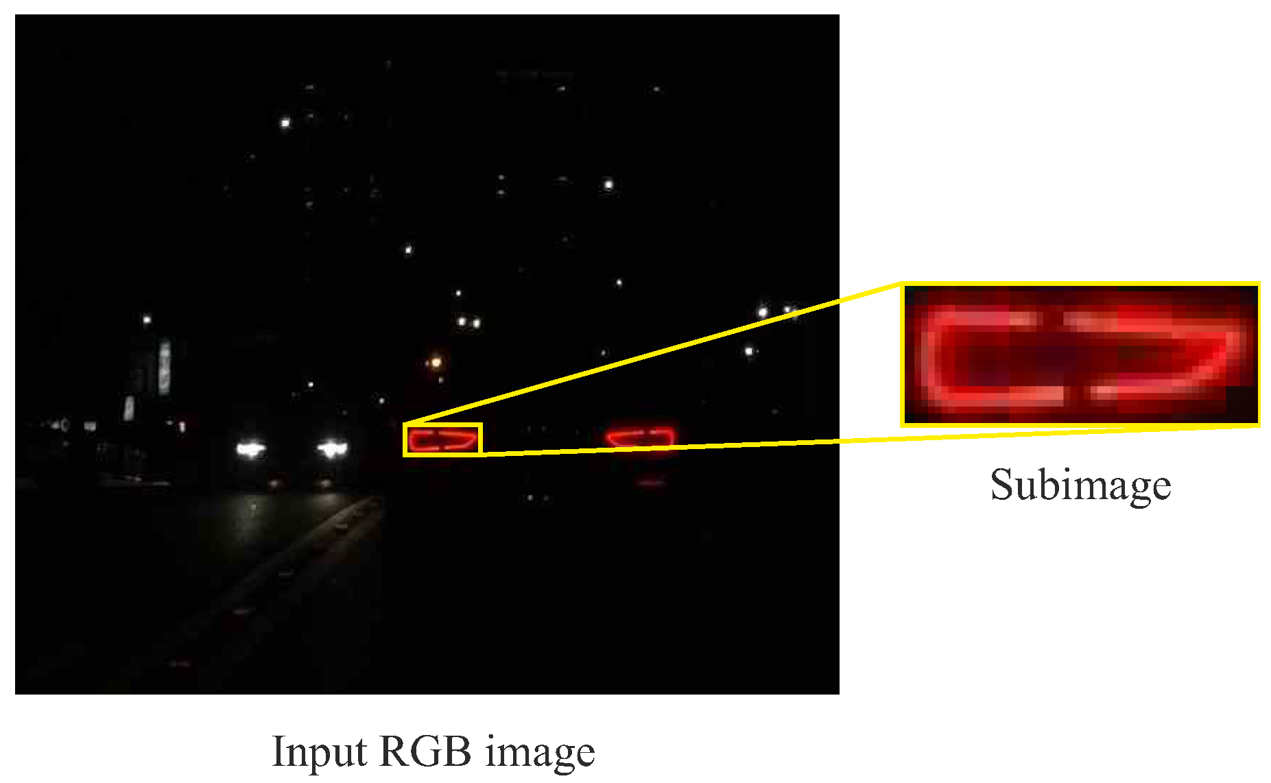
2.3. Headlight and Taillight Classification

After executing the bright blob segmentation process, the contours of bright blobs are retrieved and the location of each bright blob is determined by the position of the bounding box surrounding the contour. The position of a bounding box is defined by the left, top, right, and bottom coordinates. In this section, to remove the nonvehicle illuminant objects and identify vehicle lights, the pre-trained classifier is applied to the extracted bright blobs. 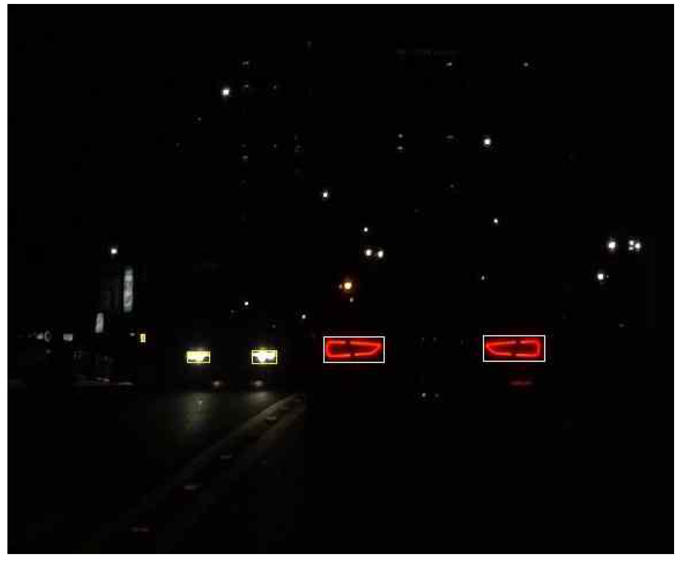First, the position of the bounding box surrounding the extracted bright blob is used to extract a subimage from the input RGB image (see Figure 7). Then, the combined features of the bright blob are calculated by using the feature extraction process presented in Section 2.1. Finally, the pre-trained classifier is used to assign a class label (headlight, taillight, or nuisance) to the combined features. The result of the classification process applied to an input RGB image is depicted in Figure 8. In Figure 8, headlights and taillights are marked by yellow and white rectangles, respectively.

2.4. Headlight and Taillight Tracking

To refine the detection results and facilitate the vehicle light pairing and vehicle tracking steps, this section presents a vehicle light tracking mechanism by considering spatiotemporal information in consecutive images. After performing the headlight and taillight classification, a headlight set and a taillight set that include the positions of bounding boxes surrounding vehicle lights are retrieved. Although the results of the previous step still contain false positives, they are going to be eliminated in subsequent steps. Because the light tracking, light pairing, and vehicle tracking mechanisms are all applied equally to both headlights and taillights, the term “vehicle lights” is used and implicitly understood as headlights and taillights.

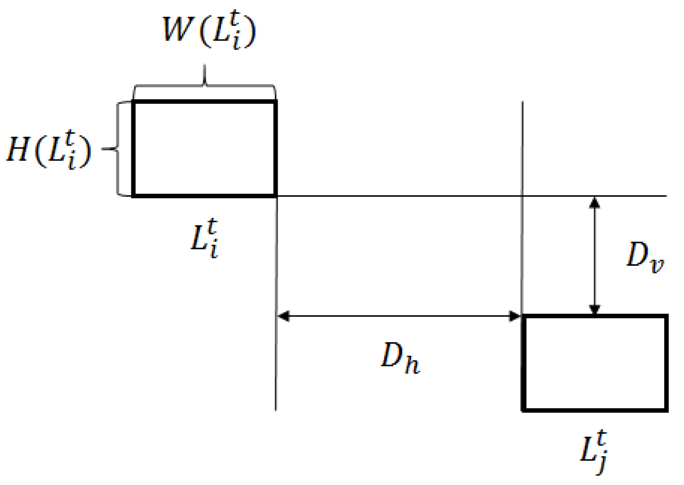
To depict the light tracking process, the following terms are first defined:

• $L_i^t(i=1,2,...,n_t)$ and $n_t$ denote the ith vehicle light in the ROI and the number of detected vehicle lights in frame t, respectively.
• $t\left(L_i^t\right),l\left(L_i^t\right),b\left(L_i^t\right),r\left(L_i^t\right)$ denote the location of vehicle light $L_i^t$, and are the top, left, bottom, and right coordinates of the bounding box enclosing $L_i^t$, respectively.
• The width and height of vehicle light $L_i^t$ are denoted as $W\left(L_i^t\right)$ and $H\left(L_i^t\right)$, respectively.
• The horizontal distance $D_h$ and vertical distance $D_v$ between two vehicle lights $L_i^t$ and $L_j^t$ in frame t are defined as

  $$D_h(L_i^t,L_j^t)=max\{l\left(L_i^t\right),l\left(L_j^t\right)\}-min\{r\left(L_i^t\right),r\left(L_j^t\right)\}$$

  (1)

  $$D_v(L_i^t,L_j^t)=max\{t\left(L_i^t\right),t\left(L_j^t\right)\}-min\{b\left(L_i^t\right),b\left(L_j^t\right)\}$$

  (2)
  The value of the distance is negative if two vehicle lights are overlapped in the horizontal or vertical projection.
• The degrees of overlap between the horizontal projections or vertical projections of two vehicle lights $L_i^t$ and $L_j^t$ in frame t are

  $$O_h(L_i^t,L_j^t)=\frac{-D_h(L_i^t,L_j^t)}{min\{W\left(L_i^t\right),W\left(L_j^t\right)\}}$$

  (3)

  $$O_v(L_i^t,L_j^t)=\frac{-D_v(L_i^t,L_j^t)}{min\{H\left(L_i^t\right),H\left(L_j^t\right)\}}$$

  (4)

The defined terms are illustrated in Figure 9.

To obtain information including the position, size, and velocity of the same vehicle light in subsequent frames, a light tracker is initialized if a vehicle light appears for the first time in the ROI. Let $T{L}_i^t=<L_i^1,L_i^2,...,L_i^t>$ denote the light tracker representing for the trajectory of $L_i^t$. The light tracker $T{L}_i^t$ tracks the vehicle light $L_i^t$ appearing from the first frame to frame t. ${\mathit{L}}^{\mathit{t}}$ denotes the set of detected vehicle lights in frame t. ${\mathit{TL}}^{\mathit{t}-\mathbf{1}}$ denotes the set of light trackers in frame $t-1$. Based on the condition in the study [6], which tracks vehicle headlights in a traffic surveillance system, two detected vehicle lights in two consecutive frames belong to one light tracker if their bounding boxes overlap to each other. Applying this condition for tracking vehicle taillights, the system is still able to track taillights, whether the preceding vehicles are moving at high or low speed. However, applying the condition for tracking vehicle headlights, the system may fail when the oncoming vehicle’s velocity is higher than 50 km/h. Therefore, a modified version of the tracking mechanism in the study [3] is presented in this section. First, the overlapping score $S_0$ of two vehicle lights (two bounding boxes) $L_i^t$ and $L_j^{t^{\prime }}$ is defined, where these lights are detected in different frames t and $t^{\prime }$.

$$S_0(L_i^t,L_j^{t^{\prime }})=\frac{A(L_i^t\cap L_j^{t^{\prime }})}{max\{A\left(L_i^t\right),A\left(L_j^{t^{\prime }}\right)\}}$$

(5)

where A is the area of the bounding box enclosing the light region. $S_0$ is used to determine the tracking state of newly detected vehicle lights in the incoming frame. It is assumed that the time interval between two consecutive frames is short (33ms for 30 frames per second), such that the vehicle velocity does not change significantly. Therefore, the motion information is used to predict the position of an incoming vehicle light. For a vehicle light that has been tracked in at least two frames, its motion vector can be calculated as follows:

$$\left\{\begin{array}{c}v{x}_i^{t-1}=l\left(T{L}_i^{t-1}\right)-l\left(T{L}_i^{t-2}\right)\hfill \\ v{y}_i^{t-1}=t\left(T{L}_i^{t-1}\right)-t\left(T{L}_i^{t-2}\right)\hfill \end{array}\right.$$

(6)

The motion vector is equal to 0 when the vehicle light appears for the first and second times. Let ${\widehat{TL}}_i^{t-1}$ denote the predicted position of the vehicle light tracker $T{L}_i^{t-1}$ in the next frame:

$$\left\{\begin{array}{c}t\left({\widehat{TL}}_i^{t-1}\right)=t\left(T{L}_i^{t-1}\right)+v{y}_i^{t-1}\hfill \\ l\left({\widehat{TL}}_i^{t-1}\right)=l\left(T{L}_i^{t-1}\right)+v{x}_i^{t-1}\hfill \\ b\left({\widehat{TL}}_i^{t-1}\right)=b\left(T{L}_i^{t-1}\right)+v{y}_i^{t-1}\hfill \\ r\left({\widehat{TL}}_i^{t-1}\right)=r\left(T{L}_i^{t-1}\right)+v{x}_i^{t-1}\hfill \end{array}\right.$$

(7)

In the light tracking process, the vehicle light tracker might be in one of three possible states:

• Update: if a detected vehicle light $L_i^t\in {\mathit{L}}^{\mathit{t}}$ in the current frame t matches a predicted position ${\widehat{TL}}_j^{t-1}$ of an existing tracker $T{L}_j^{t-1}\in {\mathit{TL}}^{\mathit{t}-\mathbf{1}}$ in the previous frame. Then, the tracker $T{L}_j^t$ is associated with $L_i^t$ and the tracker is added to the set of light trackers ${\mathit{TL}}^{\mathit{t}}$ the in current frame. The matching condition is

  $$S_0(L_i^t,{\widehat{TL}}_j^{t-1})>{\tau }_m$$

  (8)

  where ${\tau }_m$ is a matching threshold for verifying whether $L_i^t$ can be associated with $T{L}_j^{t-1}$. The value of ${\tau }_m$ is chosen experimentally as 0.2.
• Appear: if a detected vehicle light $L_i^t\in {\mathit{L}}^{\mathit{t}}$ in the current frame t does not match any predicted positions ${\widehat{TL}}_j^{t-1}$ of existing trackers $T{L}_j^{t-1}\in {\mathit{TL}}^{\mathit{t}-\mathbf{1}}$ in the previous frame. Then, a new light tracker is created and it is added to the set of light trackers ${\mathit{TL}}^{\mathit{t}}$ in the current frame.
• Disappear: if a predicted position ${\widehat{TL}}_j^{t-1}$ of existing tracker $T{L}_j^{t-1}\in {\mathit{TL}}^{\mathit{t}-\mathbf{1}}$ cannot be matched by any newly detected vehicle light $L_i^t\in {\mathit{L}}^{\mathit{t}}$ in the current frame t. Because the existing tracker may sometimes be temporarily occluded, the system keeps tracking this tracker in three consecutive frames. While the tracker $T{L}_j^{t-1}$ has temporarily disappeared, its position is updated by using Equation (7). Otherwise, if the tracker $T{L}_j^{t-1}$ cannot be matched for more than three consecutive frames, it is considered to have disappeared and is removed from the set of light trackers ${\mathit{TL}}^{\mathit{t}}$.

2.5. Headlight Pairing and Taillight Pairing

After performing the headlight and taillight tracking process, the set of vehicle light trackers is retrieved. As the vehicle lights of one vehicle are located in pairs and symmetrical, the light tracker set is used to determine the position of on-road vehicles by pairing the vehicle lights. Existing works [7,19,20] only use the spatial features within one frame, such as the area, width, height, vertical coordinate, and correlation, to check the similarity between two vehicle lights; these features are not sufficient for pairing lights. When the multiple vehicles in front are moving at the same distances from the host vehicle, incorrect light pairing may occur because the spatial features of the lights in these vehicles are similar. To reduce the false detection rate, a light pairing method using spatiotemporal information is proposed. The proposed light pairing method is separated into two stages: potential light pair generation and light pair verification.

To generate the set of candidate light pairs, the pairing criteria are given as follows:

• Two vehicle lights are highly overlapped in vertical projections:

  $$O_v(T{L}_i^t,T{L}_j^t)>{\tau }_{vp}$$

  (9)
• Two vehicle lights have similar heights:

  $$\frac{min\{H\left(T{L}_i^t\right),H\left(T{L}_j^t\right)\}}{max\{H\left(T{L}_i^t\right),H\left(T{L}_j^t\right)\}}>{\tau }_h$$

  (10)
• The ratio of pair width to pair height must satisfy the following condition:

  $${\tau }_{WH1}\le \frac{max\{r\left(T{L}_i^t\right),r\left(T{L}_j^t\right)\}-min\{l\left(T{L}_i^t\right),l\left(T{L}_j^t\right)\}}{max\{b\left(T{L}_i^t\right),b\left(T{L}_j^t\right)\}-min\{t\left(T{L}_i^t\right),t\left(T{L}_j^t\right)\}}\le {\tau }_{WH2}$$

  (11)

In the criteria ${\tau }_{vp},{\tau }_h,{\tau }_{WH1},$ and ${\tau }_{WH2}$ are the thresholds that determine the characteristics of pairing vehicle lights. These values are statistically chosen as 0.7, 0.7, 2.0, and 14.0, respectively.

The result of the first stage is the set of candidate light pairs, but this set may include some falsely detected pairs because one vehicle light can be shared in more than one pair. Therefore, light pair verification is performed to remove the false pairs.

To reduce the false pairs, a pairing score of the candidate light pair is used to perform a comparison between the conflicting pairs. Among the conflicting pairs, the pair with the highest pairing score is retained to describe a vehicle, and the other pairs are removed from the candidate pair set. The pairing score $S_p$ is a combination of spatiotemporal features of two vehicle lights ($T{L}_i^t$ and $T{L}_j^t$) in a pair, including the number of tracked frames, displacement, size, and correlation. It is defined as follows:

$$\begin{array}{c}{S}_p=w_0·r_t+w_1·r_d+w_2·r_s+w_3·r_{corr}\\ r_t=\frac{min\left\{\right|T{L}_i^t|,|T{L}_j^t\left|\right\}}{max\left\{\right|T{L}_i^t|,|T{L}_j^t\left|\right\}}\\ \left\{\begin{array}{c}{r}_d=\frac{min(d_i,d_j)}{max(d_i,d_j)}\hfill \\ d_i=\sum _{k=t-min(3,|T{L}_i^t\left|\right)}^t\sqrt{{\left(v{x}_i^k\right)}^2+{\left(v{y}_i^k\right)}^2}\hfill \\ d_j=\sum _{k=t-min(3,|T{L}_j^t\left|\right)}^t\sqrt{{\left(v{x}_j^k\right)}^2+{\left(v{y}_j^k\right)}^2}\hfill \end{array}\right.\\ r_s=\frac{1}{2}\times \{\frac{min\{W\left(T{L}_i^t\right),W\left(T{L}_j^t\right)\}}{max\{W\left(T{L}_i^t\right),W\left(T{L}_j^t\right)\}}+\frac{min\{H\left(T{L}_i^t\right),H\left(T{L}_j^t\right)\}}{max\{H\left(T{L}_i^t\right),H\left(T{L}_j^t\right)\}}\}\end{array}$$

(12)

where $r_t$ is the ratio of the number of tracked frames of two vehicle lights; $r_d$ is the ratio of the total displacements d of vehicle lights ($T{L}_i^t$ and $T{L}_j^t$) in the four most recent frames. As both lights in a pair should move coherently in time, their motion vectors are used to calculate the displacements; $r_s$ is the ratio of the sizes of two vehicle lights; $r_{corr}$ is the correlation between histograms of vehicle lights $T{L}_i^t$ and $T{L}_j^t$. Herein, the Bhattacharyya coefficient [13] is used to compare the 3-D histograms of the left and right lights.

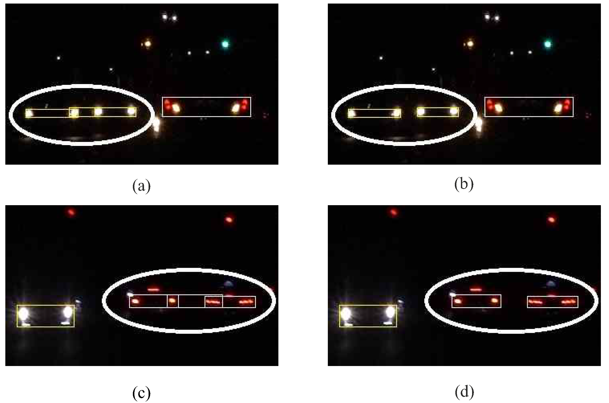
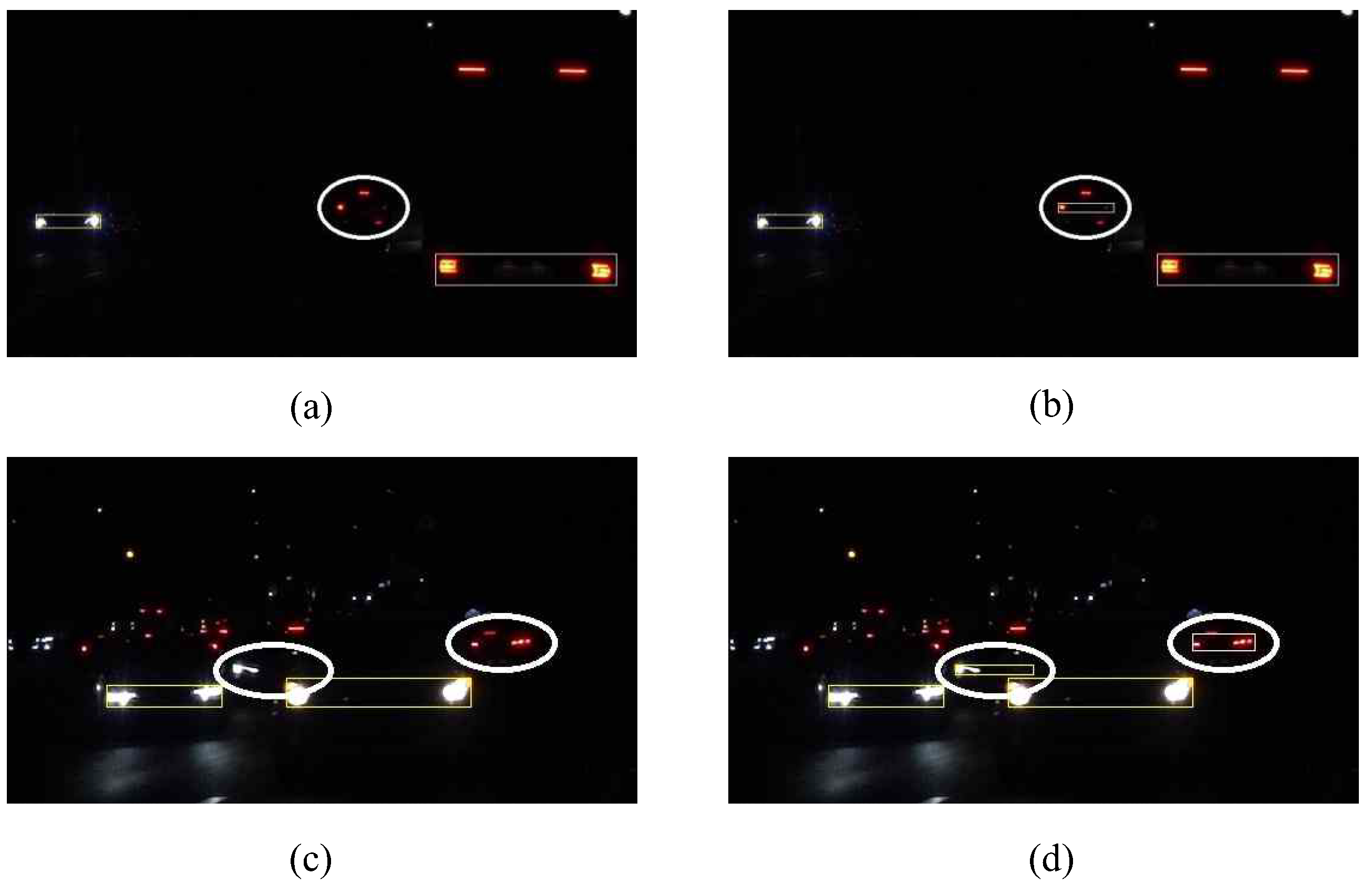
In Equation (12), the coefficients $w_0,w_1,w_2,$ and $w_3$ are experimentally chosen as 0.2, 0.2, 0.3, and 0.3, respectively. The results of light pair verification are illustrated in Figure 10. After dismissing the conflicting pairs by using the pairing score, a set of light pairs that describe the vehicles in front is retrieved and all the light trackers that are not used for pairing are retained for processing in the next phase.

2.6. Vehicle Tracking with Occlusion Handling

In the previous section, a light pairing process is proposed to find all the possible vehicles in front of the host vehicle, which it can reduce the falsely detected vehicles. On the other hand, missed pairings still occur and cannot be fixed if the system only considers vehicle detection in single frames. Missed detection happens because of several problems, which may cause either the disappearance or the distorted appearance (size, shape, or color) of one lamp in a light pair. The following problems may lead to the pairing failure: (1) partial vehicle occlusion; (2) two vehicle lights of two different vehicles are detected as one connected region when one vehicle is too close to another vehicle; (3) left-turning or right-turning vehicles; (4) blooming effect of only one light in oncoming vehicles. To solve these problems, a vehicle tracking method with occlusion handling is proposed. In the vehicle tracking process, the detection results are refined by associating the spatiotemporal features of vehicles in sequential frames. It is assumed that a pair of vehicle lights form a vehicle, such that any vehicles that have two light pairs will be put into the post-processing step to group two pairs into one pair. To facilitate describing the vehicle tracking process, the following terms are defined:

• ${\mathit{P}}^{\mathit{t}}=\{P_i^t=(P_i^t\left(1\right),P_i^t\left(2\right)|P_i^t\left(1\right)\mathrm{and}{P}_i^t\left(2\right)\in {\mathit{TL}}^{\mathit{t}},l\left(P_i^t\left(1\right)\right)<l\left(P_i^t\left(2\right)\right),i=(1,...,n_p^t)\}$ and ${\mathit{RTL}}^{\mathit{t}}$ denote the set of light pairs and the remaining light trackers retrieved from the light pairing step, respectively.
• $T{P}_i^t=<P_i^1,P_i^2,...,P_i^t>$ denotes the light pair tracker representing for the trajectory of light pair $P_i^t$.
• The location of light pair $P_i^t$ is determined by the bounding box of $P_i^t$:

  $$\left\{\begin{array}{c}t\left(P_i^t\right)=min\left\{t\right(P_i^t\left(1\right),t\left(P_i^t\left(2\right)\right\}\hfill \\ l\left(P_i^t\right)=min\left\{l\right(P_i^t\left(1\right),l\left(P_i^t\left(2\right)\right\}\hfill \\ r\left(P_i^t\right)=max\left\{r\right(P_i^t\left(1\right),r\left(P_i^t\left(2\right)\right\}\hfill \\ b\left(P_i^t\right)=max\left\{b\right(P_i^t\left(1\right),b\left(P_i^t\left(2\right)\right\}\hfill \end{array}\right.$$

  (13)
• ${\mathit{TP}}^{\mathit{t}-\mathbf{1}}=\left\{T{P}_j^{t-1}\right|j=(1,...,n_{pt}^{t-1})\}$ denotes the set of light pair trackers in the previous frame $t-1$

In the vehicle tracking process, a light pair tracker might be in one of four possible states:

• Update: if a light pair $P_i^t\in {\mathit{P}}^{\mathit{t}}$ in the current frame t matches a light pair tracker $T{P}_j^{t-1}\in {\mathit{TP}}^{\mathit{t}-\mathbf{1}}$ in the previous frame $t-1$. Then, the light pair tracker $T{P}_j^t$ is associated with $P_i^t$ and it is added to the set of light pair trackers ${\mathit{TP}}^{\mathit{t}}$ in the current frame. The matching condition for light pair is defined based on the overlapping score in Equation (5) and the ratio of pair widths of two frames $t-1$ and t:

  $$\left\{\begin{array}{c}{S}_0(P_i^t,T{P}_j^{t-1})>{\tau }_{mp}\hfill \\ \frac{min\{W\left(P_i^t\right),W\left(T{P}_j^{t-1}\right)\}}{max\{W\left(P_i^t\right),W\left(T{P}_j^{t-1}\right)\}}>{\tau }_{mpw}\hfill \end{array}\right.$$

  (14)

  where ${\tau }_{mp}$ and ${\tau }_{mpw}$ are the matching thresholds for verifying whether $P_i^t$ can be associated with $T{P}_j^{t-1}$. The values of ${\tau }_{mp}$ and ${\tau }_{mpw}$ are chosen experimentally as 0.3 and 0.7, respectively.
• Appear: if a light pair $P_i^t\in {\mathit{P}}^{\mathit{t}}$ in the current frame t does not match any light pair trackers $T{P}_j^{t-1}\in {\mathit{TP}}^{\mathit{t}-\mathbf{1}}$ in the previous frame $t-1$. Then, a new light pair tracker $T{P}_i^t$ is created and it is added to the set of light pair trackers ${\mathit{TP}}^{\mathit{t}}$ in the current frame.
• Disappear: a light pair tracker is determined to have disappeared if it satisfies the following two conditions. First, an existing light pair tracker $T{P}_j^{t-1}\in {\mathit{TP}}^{\mathit{t}-\mathbf{1}}$ cannot be matched by any light pairs $P_i^t\in {\mathit{P}}^{\mathit{t}}$ in the current frame t. Second, the predicted positions of the left and right lights in $T{P}_j^{t-1}$ do not match any light trackers $T{L}_i^t\in {\mathit{RTL}}^{\mathit{t}}$. Thus, the light pair tracker $T{P}_j^{t-1}$ is not added to the set of light pair trackers ${\mathit{TP}}^{\mathit{t}}$ in the current frame.
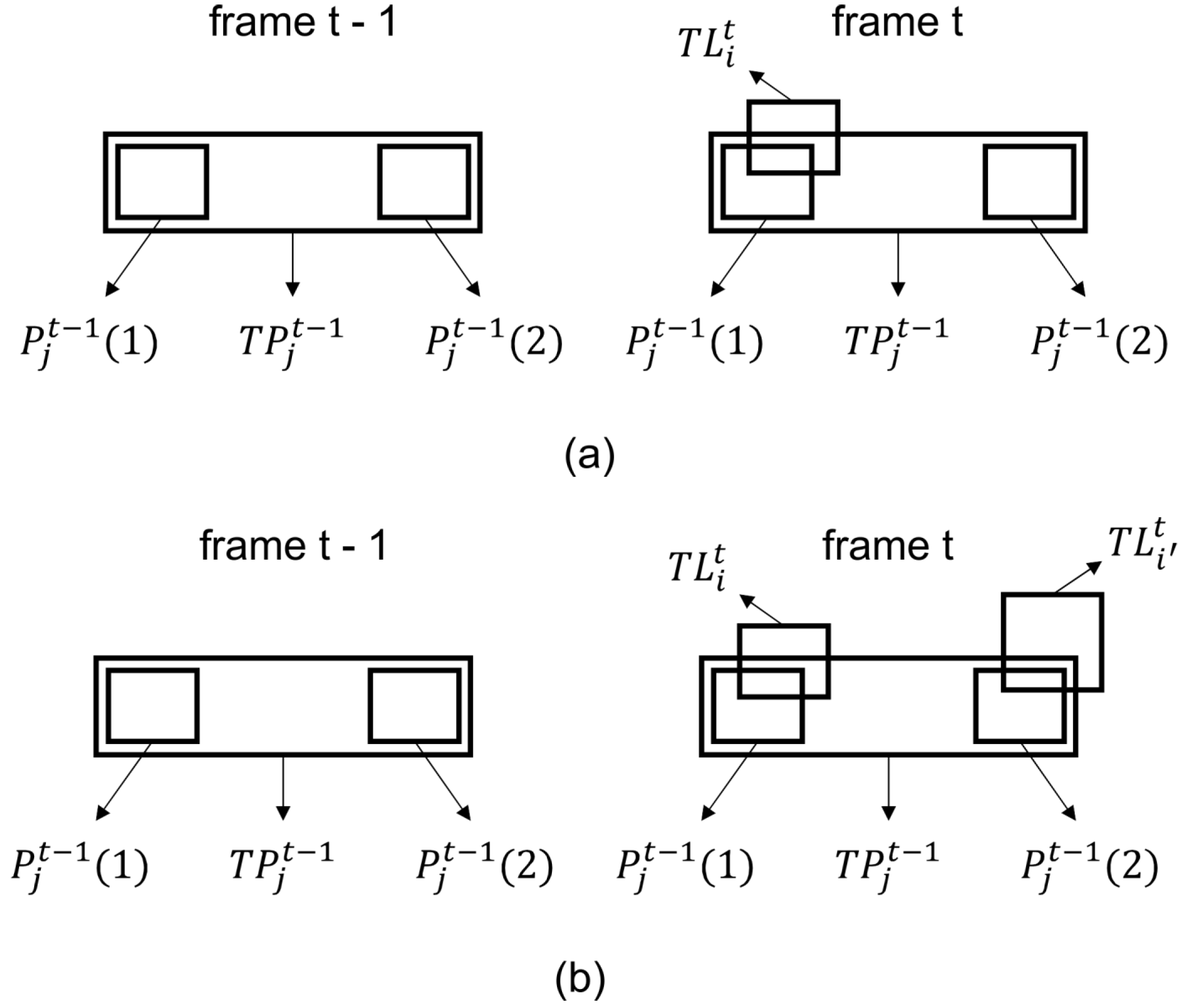
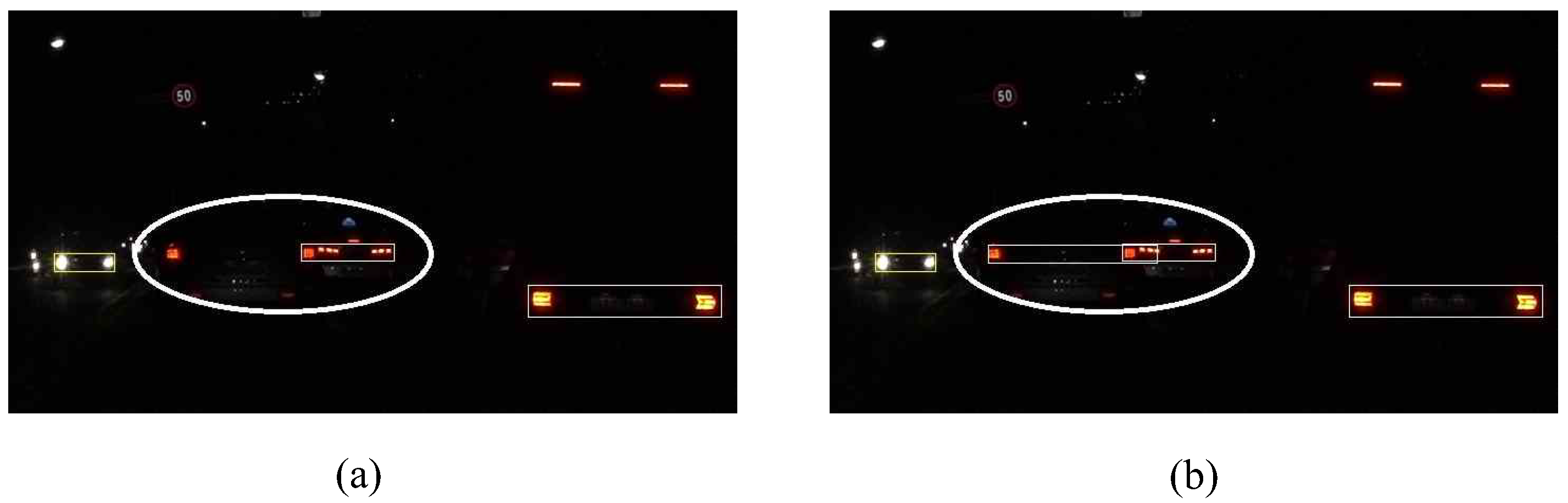
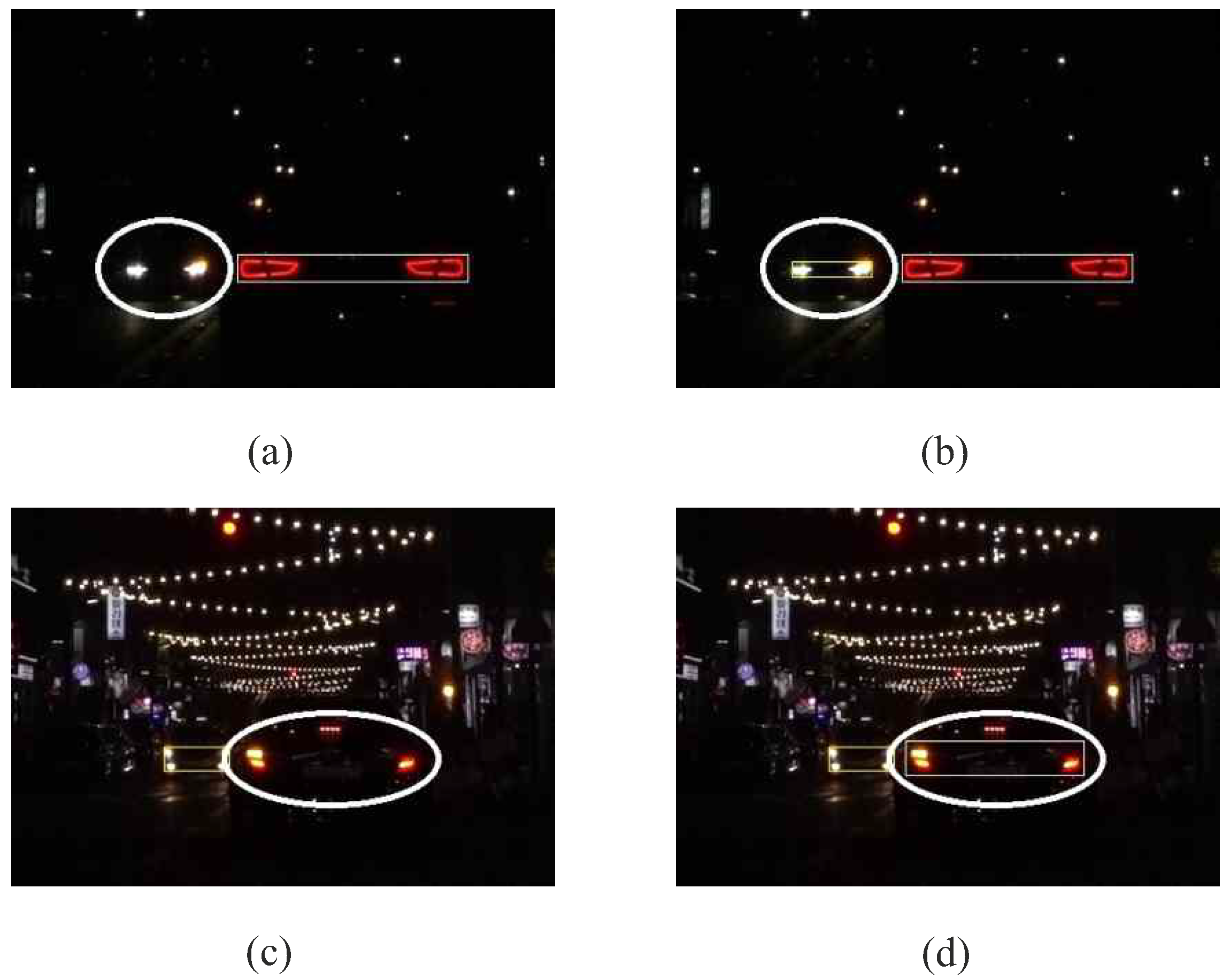
• Occlude: a light pair tracker is determined as occluded if it satisfies the following two conditions. First, an existing light pair tracker $T{P}_j^{t-1}\in {\mathit{TP}}^{\mathit{t}-\mathbf{1}}$ cannot be matched by any light pairs $P_i^t\in {\mathit{P}}^{\mathit{t}}$ in the current frame t. Second, in the case of a pairing failure due to the disappearance of one lamp in a light pair as shown in Figure 11a, the predicted position of the left or right light in $T{P}_j^{t-1}$ matches a light tracker $T{L}_i^t\in {\mathit{RTL}}^{\mathit{t}}$ (see Equation (8)). Otherwise, in the case of the distorted appearance of one lamp in a light pair as shown in Figure 11b, the predicted positions of both the left and right lights in $T{P}_j^{t-1}$ match two light trackers $T{L}_i^t\mathrm{and}T{L}_{i^{\prime }}^t\in {\mathit{RTL}}^{\mathit{t}}$. Then, depending on the whether the first or second case occurs, the light pair tracker $T{P}_j^t$ is updated by associating $T{P}_j^{t-1}$ with one or two light trackers in ${\mathit{RTL}}^{\mathit{t}}$ and it is added to the set of light pair trackers ${\mathit{TP}}^{\mathit{t}}$.

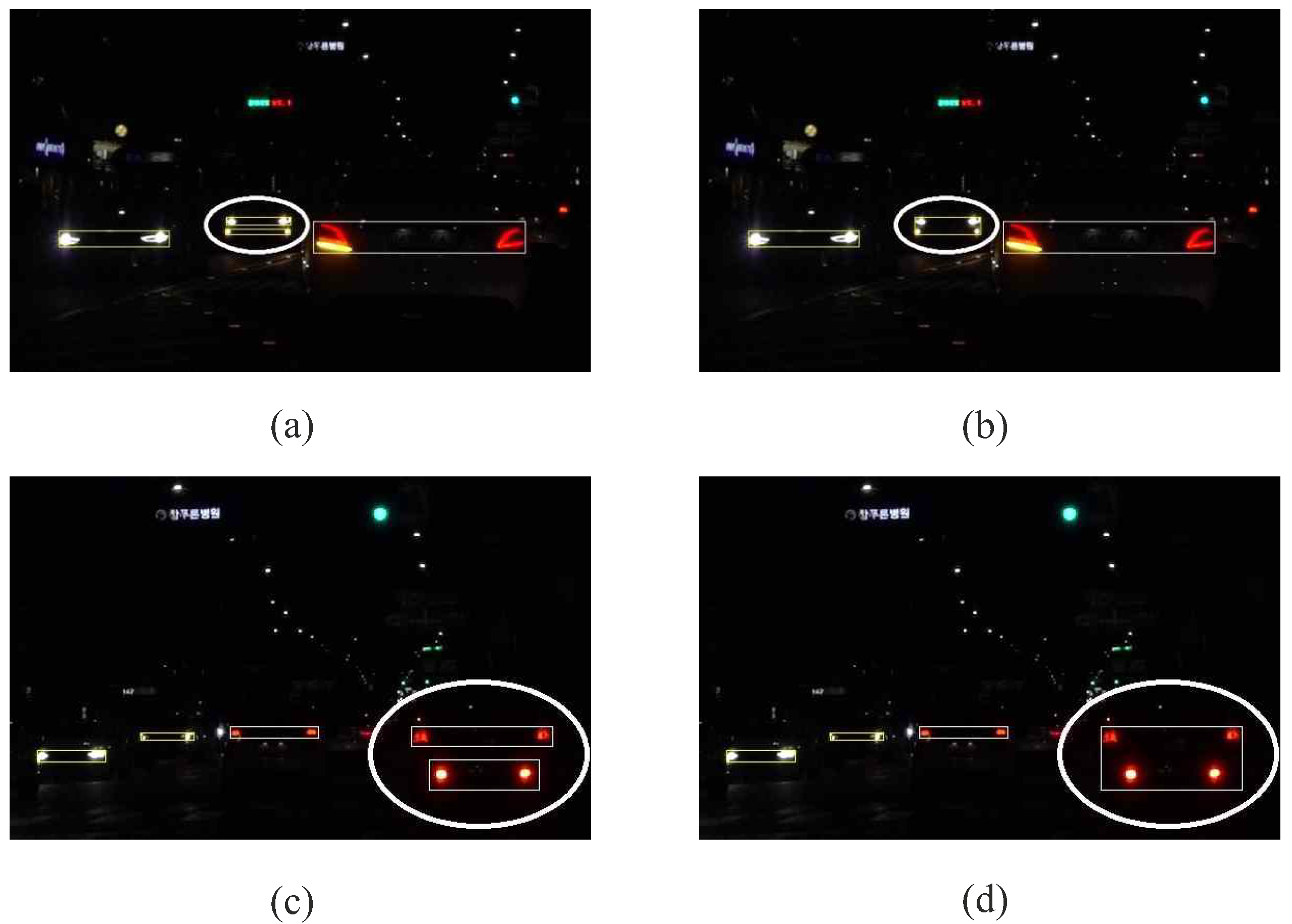
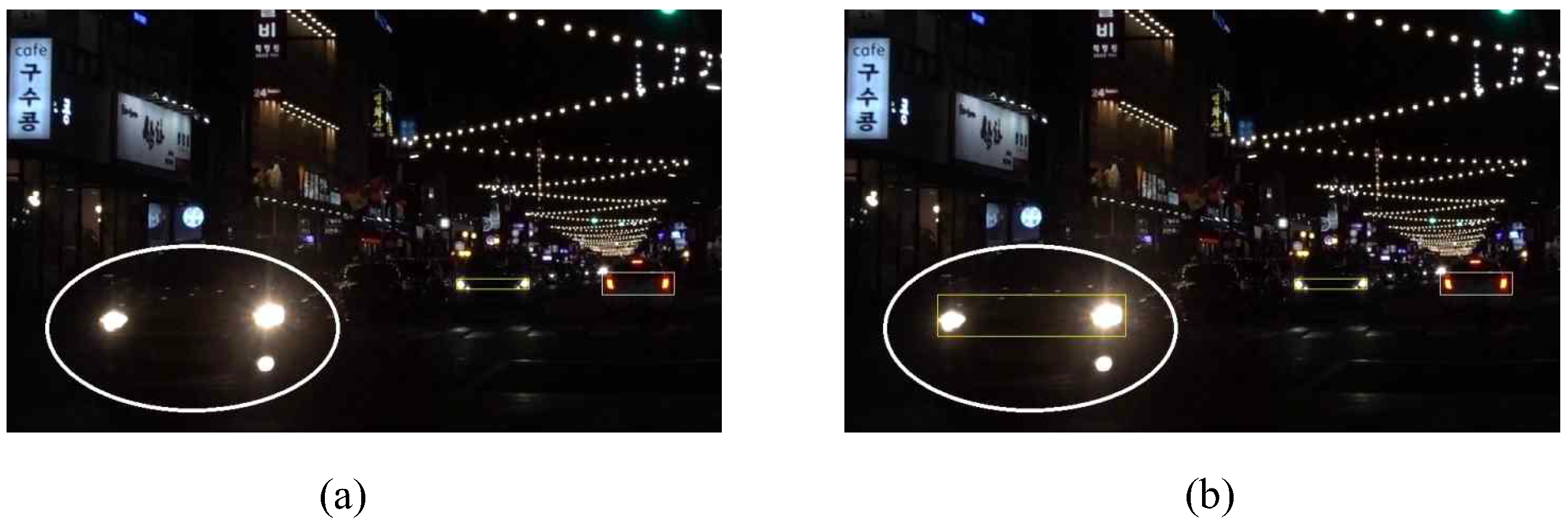
At the end of the vehicle tracking step, the set of light pair trackers ${\mathit{TP}}^{\mathit{t}}$ in the current frame t is retrieved. Next, for any vehicles with two light pairs, we apply the rules for grouping two light pairs into one pair. Two light pairs $T{P}_i^t$ and $T{P}_j^t$ are grouped into one pair if they satisfy the following rules:

• They are vertically close to each other:

  $$0<D_v(T{P}_i^t,T{P}_j^t)<2.0\times min\{H\left(T{P}_i^t\right),H\left(T{P}_j^t\right)\}$$

  (15)
• Two pairs have highly overlapped horizontal projections:

  $$O_h(T{P}_i^t,T{P}_j^t)>{\tau }_{hp}$$

  (16)
• They have similar widths:

  $$\frac{min\{W\left(T{P}_i^t\right),W\left(T{P}_j^t\right)\}}{max\{W\left(T{P}_i^t\right),W\left(T{P}_j^t\right)\}}>{\tau }_w$$

  (17)

In the post-processing step, ${\tau }_{hp}$ and ${\tau }_w$ are the thresholds for grouping multiple pairs that form one vehicle. They are chosen statistically as 0.9 and 0.7, respectively. The results of the post-processing are illustrated in Figure 12.

3. Experiment

3.1. Experimental Setup

To evaluate the proposed algorithm, we record experimental data by using a Sony DSC-RX100 V camera with a CMOS sensor. The forward-facing camera is mounted on the dashboard inside the host vehicle, as shown in Figure 13. According to the analysis of camera exposure in the study [12], the camera settings can affect to detection results of the proposed algorithm. In our experiment, exposure setting is experimentally chosen to reduce a blinking effect and blooming effect so that the captured images still keep sufficient color and shape information. The camera settings are chosen as follows: exposure time 1/100 s, lens aperture f7.1, ISO 640, resolution 1920 × 1080, 30 frames per second, and focal length 35 mm.

Depending on the road width and traffic volume [21], we choose two scenarios, which are two-lane and four-lane urban roads at night for recording traffic videos. The recorded data used in the experiment contain 9200 test images, which are separated into 18 video segments (with an average of 500 frames per video segment). These video segments are collected in various traffic situations, such as partial vehicle occlusion, turning vehicles, driving on curvy roads, and passing maneuvers.

In this study, we adopt the Jaccard coefficient [10,22] for evaluating the performance of the proposed algorithm. The ground-truth of vehicles in the dataset is labeled manually by human observation. The Jaccard coefficient J for one video is defined as:

$$J=\frac{{\sum }_{t=1}^{n}T{P}_t}{{\sum }_{t=1}^n(T{P}_t+F{P}_t+F{N}_t)}$$

(18)

where n is total number of frames in a video segment, and $T{P}_t$ (true positive), $F{P}_t$ (false positive), and $F{N}_t$ (false negative) are the total number of detected vehicles, falsely detected vehicles, and missed vehicles in frame t, respectively.

3.2. Results and Discussion

3.2.1. Headlight and Taillight Detection

As presented in Section 2.1, the proposed classifier is used to classify whether the bright blob is a headlight, taillight, or nuisance light. To train the classifier, we use a dataset containing 300 headlights, 300 taillights, and 300 negative images. All the training images are normalized to a fixed size of 20 × 20 pixels. Then, to evaluate the classification, we split the dataset into 80% for training and 20% for testing. Using the precision (Equation (19)) and recall (Equation (20)) metrics, the performance of the proposed and existing classifiers are listed in

Table 1. Classification results.

Class	Without Color Feature		With Color Feature
	Precision (%)	Recall (%)	Precision (%)	Recall (%)
Headlight	95	95	100	100
Taillight	85	89	95	100
Negative	85	81	100	95

. It can be seen that a classifier is unable to classify both headlights and taillights well if it is only trained with Haar features. The evaluation results are improved significantly by combining two types of features.

$$precision=\frac{truepositive}{truepositive+falsepositive}$$

(19)

$$recall=\frac{truepositive}{truepositive+falsenegative}$$

(20)

3.2.2. Vehicle Detection and Tracking

In this section, we compare the performance of an existing algorithm [7] (without occlusion handling) and the proposed algorithm (with occlusion handling) under two scenarios of two-lane and four-lane urban roads. To describe the detected vehicles in the images, the preceding vehicles are marked as white rectangles and the oncoming vehicles are marked as yellow rectangles.

Table 2. Vehicle detection results for test videos of two-lane urban roads.

Test Videos	Jaccard Coefficient of Oncoming Vehicles (Headlights)		Jaccard Coefficient of Preceding Vehicles (Taillights)
	Without Occlusion Handling (%)	With Occlusion Handling (%)	Without Occlusion Handling (%)	With Occlusion Handling (%)
Video 1	81.56	96.16	94.12	98.6
Video 2	72.69	96	93.59	99.2
Video 3	76.37	94.75	88.43	97.35
Video 4	85.19	95.51	98.76	98.76
Video 5	88.73	94.39	93.67	96.07
Video 6	79.35	96.54	97.19	98
Video 7	86.28	95.94	85.08	98.13
Video 8	73.4	93.33	84.19	98.36
Video 9	73.19	92.19	93.45	99.51
Video 10	85.21	91.63	78.32	97.59
Average result	80.2	94.64	90.68	98.16

shows the quantitative evaluation results for the test videos recorded on two-lane urban roads. It is clear that the system performance is improved significantly in both oncoming and preceding vehicle detection when the occlusion handling mechanism is applied. As presented in the vehicle tracking section, missed detections may occur because of the disappearance or the distorted appearance of one lamp in a light pair. In the two-lane scenario, for both preceding and oncoming vehicles, the typical situation that causes vehicle detection failure involves turning vehicles. When the front vehicle turns left or right, the appearance of a vehicle light is distorted, which breaks the pre-defined conditions for light pairing. Figure 14 illustrates the comparative results with and without occlusion handling in turning situations. Furthermore, for oncoming vehicles, the blooming effect of only one light in a light pair sometimes occurs, which also causes failed detection. Figure 15 shows the successful vehicle detection of the proposed method compared with an existing work when the blooming effect occurs.

Table 3. Vehicle detection results for test videos of four-lane urban roads.

Test Videos	Jaccard Coefficient of Oncoming Vehicles (Headlights)		Jaccard Coefficient of Preceding Vehicles (Taillights)
	Without Occlusion Handling (%)	With Occlusion Handling (%)	Without Occlusion Handling (%)	With Occlusion Handling (%)
Video 1	83.84	91.28	71.33	93.9
Video 2	84.48	92.29	81.18	95.18
Video 3	86.91	89.61	85.45	89.37
Video 4	71.65	91.57	83.21	93.69
Video 5	70.67	85.71	88.92	96.03
Video 6	67.59	94.25	78.72	95.94
Video 7	81.56	82.13	73.87	93.34
Video 8	74.19	91.71	78.06	97.82
Average result	77.61	89.82	80.09	94.41

shows the quantitative evaluation results for the test videos recorded on four-lane urban roads. As with the results in the two-lane scenario, the vehicle detection performance is significantly enhanced when the proposed method is applied for detecting both oncoming and preceding vehicles. Compared to a two-lane road, the width and traffic volume of a four-lane road are both larger and thus there are various situations that may cause incorrect vehicle detection (missed detection or false positive). In addition to the situations mentioned for the two-lane scenario, partial vehicle occlusion occasionally happens owing to the viewpoint of the host vehicle’s camera or the passing maneuver of vehicles in front. Figure 16 shows vehicle detection results for partial vehicle occlusion. As with the occlusion handling mechanism, the proposed method uses the information of the vehicle that has been tracked in the previous frame to update the new vehicle position, even if the light pair process for the occluded vehicle has failed.

Occasionally, when one vehicle is moving very close to another vehicle, one of the two vehicles may be missed in the detection because two adjacent vehicle lights are detected as one vehicle light, as shown in Figure 17a. However, the proposed algorithm is still able to obtain both vehicles, as shown in Figure 17b.

Table 4. Average vehicle detection results of two-lane and four-lane videos.

Scene	Jaccard Coefficient of Oncoming Vehicles (Headlights)		Jaccard Coefficient of Preceding Vehicles (Taillights)
	Without Occlusion Handling (%)	With Occlusion Handling (%)	Without Occlusion Handling (%)	With Occlusion Handling (%)
Two lanes	80.2	94.64	90.68	98.16
Four lanes	77.61	89.82	80.09	94.41
Average result	78.9	92.23	85.39	95.81

shows the average vehicle detection results for both two-lane and four-lane scenarios. With occlusion handling, the proposed method has enhanced the system performance effectively; the average detection result for preceding vehicles is 92.23% and that for oncoming vehicles is 95.81%. The results of vehicle detection based on headlights are lower than those for taillights, as the blooming effect frequently occurs for headlights. Because of that, the size, shape, and illuminance of headlights are unstable in the captured images. As a result, false pairing between adjacent vehicles occurs because a light in a vehicle may be paired with a light in another vehicle, especially in the four-lane scenario. Additionally, the detection results for the two-lane scenario are higher than those in the four-lane scenario, because many situations that can cause incorrect pairing occur in the four-lane scenario.

Although the performance of the proposed method is quite effective, there are still several limitations of our work. (1) Motorcycles are not considered in this study. (2) Our method can perform well with partial vehicle occlusion, but still cannot solve complete vehicle occlusion. (3) False detections occasionally occurs because of false pairing, especially in heavy traffic.

4. Conclusions

In this paper, a nighttime vehicle detection system for detecting both oncoming vehicles and preceding vehicles based on headlights and taillights is proposed. Initially, a bright blob segmentation is performed to extract all the possible regions that may be vehicle lights. Then, a machine-learning-based method is proposed to classify headlights and taillights, and to remove false detections in the captured image. Next, each vehicle light is tracked in subsequent frames by using a light tracking process. As one vehicle is indicated by one or two light pairs, a modified light pairing process using spatiotemporal information is applied to the sets of detected headlights and taillights to determine the positions of the potential vehicles. Finally, the vehicle tracking process is applied to refine the vehicle detection rate under various complex situations on the road. The experimental results demonstrate that the proposed method significantly improves vehicle detection rate by identifying the vehicles in some situations that previous studies cannot solve.

It is interesting to apply the proposed algorithm to the daytime condition in the future. We also investigate various weather scenarios, such as rainy or cloudy conditions. Furthermore, motorcycle detection and tracking will be examined for integration into the current system.