Novel Deep Level Image State Ensemble Enhancement Method for M87 Imaging

Abstract

Standard spatial domain filters fail to adequately denoise and enhance the contrast of an image. These filters have drawbacks like oversmoothing, diminished texture, and lack of generative capabilities. This paper proposes a new method of image reconstruction, Image State Ensemble Enhancement (ISEE), based on our previous work, Image State Ensemble Decomposition (ISED). Deep level ISEE and ISED have been developed to produce a class of filters that can address these issues. Full-reference and no-reference quality metrics are used to assess the image, and the full reference metrics showed a marked improvement, while the no-reference metrics were often better than the test image. The test image was taken from the Spitzer Space Telescope (SST), and ISEE reconstruction yielded improved structural detail over that of ISED and the original test image. Glare and noise were reduced in a narrow bandwidth, which led to the discovery of a vortex-shaped structure and an outburst in M87′s dusty infrared core. The vortex is located over M87′s visible core and black hole. This is verified with an SST and Hubble Space Telescope (HST) overlay, ISEE processed image. A counter-jet channel was also discovered, and it appears to be the path of the unobservable superluminal counter-jet.

1. Introduction

This paper investigates a new method to enhance features and improve color image processing. The Image State Ensemble Enhancement (ISEE) and Image State Ensemble Decomposition (ISED) methods can denoise and enhance contrast. Although the topic we have chosen to analyze is astronomical, these methods can easily be applied to color medical imaging. Denoising and contrast enhancement are commonly applied to medical imaging and have been the subject of intense research [1]. ISED and ISEE reconstructions can denoise, enhance the contrast, and provide feature extraction. ISEE improves the full-reference metrics and narrows the bandwidth of the filter, which allows for the extraction of finer details than ISED. See our unpublished histological image examples of ISED and ISEE reconstructions available online at [2] for more details.

The proposed deep level ISED and ISEE reconstructions differ from traditional types of filters. ISED and ISEE rely on some basic precepts of quantum mechanics to statistically determine and generate filtered color images based on possible image outcomes [3]. ISED and ISEE reconstructions are performed in the spatial domain. Common spatial domain filters often rely on convolution kernels or a window to modify a group of pixels [4]. Mean filtering and median filtering are common methods to smooth the image to reduce types of noise, but at the cost of adding some blurring to the image [5]. ISED and ISEE use a pixel-wise cross-channel relationship that does not suffer from blurring issues. However, the drawback to ISEE and ISED is that you must have at least two different channels to formulate the ψ-ensemble relationship. This method is designed for color images only. Various types of equalizations are also performed commonly on images. Histogram equalization redistributes the intensities of the pixels for close contrast valued images. At times, this can be a godsend, and at other times, you will end up with unrealistic oversaturated images [2]. With ISED or ISEE, oversaturation can never happen. The generated image never exceeds the intensity values of the original image, and the pixels intensities are not redistributed thought the image. ISED and ISEE reconstructions are an entirely new class of digital filters that have the ability to selectively remove small specific regions of information from the image, and the ISEE reconstruction restores part of the filtered information and generates possible narrowband filtered images. ISED and ISEE have similar characteristics to optical filters.

Our previous study used ISED to reduce unwanted effects of glare, noise reduction, and image artifacts [1]. The perceptual quality of the image was improved and made evident by lower Perception-based Image Quality Evaluator (PIQE), Natural Image Quality Evaluator (NIQE), and Blind/Referenceless Image Spatial Quality Evaluator (BRISQUE) for most ISED images. While no-reference quality metrics were improved, the full-reference quality metrics structural similarity (SSIM) index, mean-squared error (MSE), and the peak signal-to-noise ratio (PSNR) decreased—a behavior that was anticipated when performing image decomposition [1].

This paper addresses the issue of decreased performance in SSIM, MSE, and PSNR and introduces ISEE deeper decomposition levels (Ln), while presenting an image reconstruction process algorithm deemed ISEE. In the previous paper “Novel Image State Ensemble Decomposition Method for M87 Imaging”, we were able to generate ISED images that had improved no-reference image quality metrics over those of the original images provided by National Aeronautics and Space Administration (NASA). For certain generated images, there was a reduction in the noise, glare, and the filter that made it possible to observe previously unseen structures [1]. The galactic core had greater detail, and the infrared (IR) outer ring had clearer boundaries [1]. The images produced from that study were the result of a new class digital narrowband filters that can be applied to extract features in color images. In our case, the feature that we want to extract is glare and noise. As it turned out, there was a great deal of blue-biased noise in the original image. The ISED method was successful in reducing this noise, and the quantum-based equations proved to be fully functional and useful. However, this initial method has a cost. The full-reference quality metrics were lowered. The filtered portions of noise, glare, and image artefacts are the desired effect for specific ISED states.

Our new method, ISEE, takes the ISED method much further by providing deeper levels of image decomposition, where the variable n in Ln denotes the number of iterations the test image goes through in the ISED process in relation to deeper Ln. This further decomposes the image; however, more information is contained within the filter as decomposition increases. We will show this is an advantageous byproduct of the ISED process. For this study, the test image goes through six levels of decomposition (L6) and ISEE reconstruction in order to uncover never-before-seen details in the vicinity of an active galactic nuclei (AGN) that is ejected out of Virgo A’s (M87) core. The results of this paper are proof of concept and a practical application of imaging using deep Ln ISED and ISEE reconstruction. All processed test images for the deep Lns and ISEE reconstructions are available online [2].

ISEE images take a specific decomposed ISED image and combine it with the filtered image information. As the levels of decomposition increase, the information in the ISED filter plus image combine to produce a narrower band digital filter. By design, this produces higher SSIM, MSE, and PNSR. We are looking for the “sweet spot” in the image. Our main goal is to determine if we can see where the black hole is hiding and what else is hiding along with it. We are looking for structures in these galactic images that are not apparent in the original postprocessed image, but based on the previous study, we knew there was more information contained within the original image and developed ISEE as a way to extract new features while improving the full-reference quality metrics. This is applicable if the appropriate filter is selected for the ISEE reconstruction; the image evolves to become more like the original test image.

The equivalent state ISED image combined with the equivalent state ISED filter produces the original image. The same is also true for deeper Ln ISED filters and images. However, with deeper Ln ISED, the information in the decomposed image decreases, and the image information contained in the filter increases. Therefore, as a result, deeper Ln for ISED images decreases in SSIM. The ISEE reconstruction takes advantage of this transfer of information to the “filter side” of the image. For ISEE generated images, the SSIM increases in general for every additional Ln. When examining the histograms and the cumulative distribution functions (CDFs) of the ISEE images, one can clearly see that some ISEE images converge to the original image if given enough Ln and other ISEE images remain divergent. Consequently, ISED images from the previous study that had high SSIM produce the divergent case for ISEE images. The divergent case is, in part, caused by the limited amount of image information contained in the ISED filter.

The National Aeronautics and Space Administration’s (NASA’s) infrared Spitzer Space Telescope (SST) has long peered into the black abysses of our universe. SST was launched in 2003 to observe the coldest brown dwarf stars, the furthest red-shift galaxies, and uses its infrared imaging to see through the interstellar dust to discover what is hidden beneath it [6]. SST’s Infrared Array Camera (IRAC) is well suited to find AGNs, ultraluminous galaxies, superplanets, and protoplanetary discs [7]. The ability of infrared light to penetrate dust makes the test image taken from the SST ideal for multiple reasons. First, the quality of the image is high due to NASA employing some of the best scientists and engineers on the planet. Image analysts have worked their scientific wizardry and have taken this selected image to the very limits of the SST’s capability. Second, the infrared (IR) regime of the spectrum has many applications that are of interest to industry and scientific study. IR can be used in fire rescue to see through the thick smoke of a burning building and help save people that are trapped [8], medical applications such as detection of melanomas [9] and breast cancer, remote sensing by [10] satellite for oceanography [11] and meteorology [12], agriculture and food science [13], and autonomous navigation [14], just to name a few. ISED and ISEE need at least two-color bands to be implemented, depending on the sensor scheme or camera involved; however, one could feasibly apply the proposed methods to the aforementioned applications in order to construct a broad range of filters or selective enhancements to optimize the systems.

Due to deep Ln ISED and ISEE’s unique method of image decomposition and enhancement, we discovered, by observation via image processing the test image, that there is evidence for a past explosive outburst that is tangential to HST-1 and it seems to have originated from HST-1 and a structure resembling a vortex located over the vicinity of M87′s black hole and galactic center. HST-1 is a knot structure that was observed to change in luminance in the path of the eastbound superluminal jet [15]. This study also observed that on the west side of the outer dust ring, there is a linear relationship between the vortex and observed channel that is the apparent path of the superluminal counter-jet that forms the C-like shockwave structure to the west of the IR core. This jet is rendered invisible due to its relativistic Doppler shift [16]. The counter-jet channel has a linear relationship to a possible second knot, which I will refer to as HST-2. Furthermore, near the vortex is a blue C-like structure that seems to originate within the vicinity of the vortex structure, and it extends outward to follow the apparent path of the shockwave. The IR outburst is located on the northeastern portion of the IR core, and it seems to be near HST-1. Additionally, with select ISED filters and ISEE reconstruction schemes, we were able to resolve the dusty IR core, outer dust ring, and shockwaves with stunning clarity.

The clarity is due to the enhanced contrast from the combination of ISED and ISEE reconstruction. The filter reduces the blue-biased glare and noise, which enhances the contrast and informative structural details of the IR core, and the outer dust ring becomes more pronounced. The ISEE reconstruction restores a portion of the information to the image. Image quality assessments (IQAs) are shown with the corresponding images in the Results and Discussion section. Moreover, located on the southwestern portion of the dusty outer ring, there is a globular mass that appears to be feeding the black hole or perhaps was formed from another outburst from the black hole. The mass is a clump of matter like that of the globular structure that apparently obscures regions of the eastbound visible spectrum superluminal jet, perhaps a globular cluster because so many are prevalent in M87 [17]. As a final point, within M87′s dusty IR core, there appears to be a direct disturbance caused by the proximity of the supermassive black hole. In order to further analyze the findings, a Sobel filter was applied to a tighter crop of the galactic core image to produce images of the Sobel gradient magnitude, directional gradients, and gradient direction. Furthermore, image differencing with intensity scaling was used to build an additional set of images to compare the ISEE images to the original image [18]. Several overlays were also constructed from the SST ISED test image and a Hubble Space Telescope (HST) image [19]. This was done to compare the structural features of the IR chromatic ordered test image and a visible/IR chromatic ordered HST image. The overlay images are in Appendix A and will be discussed briefly. Of note, the dusty IR core, when compared in the ISEE processed HST in the overlay, shows that the IR core is offcenter and roughly aligns with the western edge of dusty IR core (SST) and the smaller visible core (HST). The IR core is much larger and encompasses HST-1. HST-1 appears to be roughly the center of the radio core and the center of the dust ring. Hence, this paper proposes a novel method of image processing while simultaneously revealing astronomical phenomena via applied deep Ln ISED and ISEE reconstruction.

The paper is organized as follows. Section 2 provides the mathematical framework to construct deep Ln ISED and ISEE images and filters. Section 3 provides an overview of the materials and methods used to generate deep Ln ISED and ISEE images. Section 4 presents the experimental results and discussion. Finally, the conclusion in Section 5 explains the impact of deep Ln ISED, ISEE, and the astronomical findings in this study.

2. Mathematics of Image State Decomposition and Enhancement

In order to produce deep Ln ISEE images, one must first perform deep Ln ISED. The notation of ISED has been modified to create what we term as deep Ln generated images and filters. As Ln increases, the SSIM, PSNR, and IMSE decreases. From our previous study, Theorem 1 is proposed.

Theorem 1.

Φ_m,n≡ The scalar probability of an ensemble of states to either succumb to wave collapse and be measured or not be detected. The regions of the wave collapse are bounded by the probability of [0, 1] [1].

$${\varphi }_{m,n}=\left[0,1\right]$$

(1)

2.1. ψ-Ensemble Matrices, for (RGB)_m,n

The ψ-ensemble matrices in (2), designed for an RGB image where ψ_m,n ≥ 0, are nonnegative ensemble matrices. For the sake of brevity in the notation, the ij index values will be removed from the following formula. The mathematics is applied pixel-wise and across the color channels to build the ψ-ensemble relations; it is of note for the sake of formalism to indicate the index notation. The m index in the following formula is the level of decomposition (Ln), and the integers 1 to 6 represent the first six levels of ISED decomposition demonstrated in this study. For clarity, the notation L6 is the sixth level of decomposition, and L3 would indicate the third level of decomposition. The n index in the following formula refers to the particular ψ-ensemble matrices ψ_m,n (state settings). The matrices in (2) are the possible ensemble relations between three color channels. R, G, and B. There can be between two to n channels for this method, but the ψ-ensemble matrices must be formulated for application-specific purposes [1]. The [0, 1] in our case is a binary decision in our study, 0 = not detected (off) and 1 = detected (on).

$$\begin{array}{l}{\psi }_{m,1,ij}^{}=\left[0,1\right]{(\mathrm{B}}_{m,ij}{-\mathrm{G}}_{m,ij}^{})\\ {\psi }_{m,2,ij}^{}=\left[0,1\right]{(\mathrm{R}}_{{}^{\mathrm{m},\mathrm{ij}}}{-\mathrm{G}}_{{}^{\mathrm{m},\mathrm{ij}}})\\ {\psi }_{m,3,ij}^{}=\left[0,1\right]{(\mathrm{R}}_{{}_{{}^{\mathrm{m},\mathrm{ij}}}}{-\mathrm{B}}_{{}^{\mathrm{m},\mathrm{ij}}})\\ {\psi }_{m,4,ij}^{}=\left[0,1\right]{(\mathrm{G}}_{{}^{\mathrm{m},\mathrm{ij}}}{-\mathrm{B}}_{{}^{\mathrm{m},\mathrm{ij}}})\\ {\psi }_{m,5,ij}^{}=\left[0,1\right]{(\mathrm{G}}_{{}^{\mathrm{m},\mathrm{ij}}}{-\mathrm{R}}_{{}^{\mathrm{m},\mathrm{ij}}})\\ {\psi }_{m,6,ij}^{}=\left[0,1\right]{(\mathrm{B}}_{{}^{\mathrm{m},\mathrm{ij}}}{-\mathrm{R}}_{{}^{\mathrm{m},\mathrm{ij}}})\end{array}$$

(2)

To clarify the notation, the example ψ_3,2j (3) is the third decomposition of the ensemble matrix, recall the pixel-wise ij indices are dropped for brevity.

$${\psi }_{3,2}^{}=\left[0,1\right]{(\mathrm{R}}_{{}^3}{-\mathrm{G}}_{{}^3}).$$

(3)

ψ_3,2 = [0, 1] (R₃-G₃) has different matrix values when compared to other Ln. To further illustrate, for this type of recursion, the L1 matrix notation would be ψ_1,2 = [0, 1] (R₁-G₁). Additionally, lower value Ln ISED images contain more information in the ψ-ensemble matrix.

2.2. Image States Ensemble Decomposition for Deep Levels (Ln)

The following Equation (4) is the basis of formulating deep Ln ISED equations and plays an integral role in the construction of ISEE image generation. This has been modified for deeper Ln and extends the notation from the previous study [3].

$$\begin{array}{l}{R}_{m,n}^{}=R\prime -\frac{1}{\sqrt{2}}({\psi }_{m,1}^{}+{\psi }_{m,2}^{}+{\psi }_{m,3}^{}+{\psi }_{m,4}^{}+{\psi }_{m,5}^{}+{\psi }_{m,6}^{})\\ G_{m,n}^{}=G\prime -\frac{1}{\sqrt{2}}({\psi }_{m,1}^{}+{\psi }_{m,2}^{}+{\psi }_{m,3}^{}+{\psi }_{m,4}^{}+{\psi }_{m,5}^{}+{\psi }_{m,6}^{})\\ B_{m,n}^{}=B\prime -\frac{1}{\sqrt{2}}({\psi }_{m,1}^{}+{\psi }_{m,2}^{}+{\psi }_{m,3}^{}+{\psi }_{m,4}^{}+{\psi }_{m,5}^{}+{\psi }_{m,6}^{})\end{array}$$

(4)

For the example of how the notation in (4) would be written for an L2 ISED image, you would use the above equation to generate the 63 balanced ISED images for the second level of decomposition using Algorithm 1 (L2), where the 63rd state S_2,63 = (RGB)’ is used to generate the image in Figure 1c. I hope to avoid as much ambiguity as possible by providing the example equation in (5). These images are different from the previous study [1]. An L6 ISED decomposition would have 36 ψ-ensemble matrices per generated channel. An L1 ISED would have 6 ψ-ensemble matrices per generated channel. In (5) below is an example of an L2 ISED that has 12 ψ-ensemble matrices per generated channel.

2.3. Example Formula for a Deep L2 ISED

The second level of decomposition (L2), where the 63rd state S_2,63 = (RGB)’. I chose to reiterate the meaning of L2 because I wish to avoid confusing the reader when involving new notation and implementing a novel image processing technique. The formula in (5) would be one possible method used to generate L2 ISED images and filters. It is used in combination with Algorithm 1 because the decomposition builds on the previous results of the lower level decompositions. So, L1 needs to be processed prior to processing L2, and the L1 results are used to build L2. This process can be used up to Ln. This is the expanded form of (4) for an L2 ISED image.

$$\begin{array}{l}{R}_{2,n}^{}=R\prime -\frac{1}{\sqrt{2}}({\psi }_{1,1}^{}+{\psi }_{1,2}^{}+{\psi }_{1,3}^{}+{\psi }_{1,4}^{}+{\psi }_{1,5}^{}+{\psi }_{1,6}^{}+{\psi }_{2,1}^{}+{\psi }_{2,2}^{}+{\psi }_{2,3}^{}+{\psi }_{2,4}^{}+{\psi }_{2,5}^{}+{\psi }_{2,6}^{})\\ G_{2,n}^{}=G\prime -\frac{1}{\sqrt{2}}({\psi }_{1,1}^{}+{\psi }_{1,2}^{}+{\psi }_{1,3}^{}+{\psi }_{1,4}^{}+{\psi }_{1,5}^{}+{\psi }_{1,6}^{}+{\psi }_{2,1}^{}+{\psi }_{2,2}^{}+{\psi }_{2,3}^{}+{\psi }_{2,4}^{}+{\psi }_{2,5}^{}+{\psi }_{2,6}^{})\\ B_{2,n}^{}=B\prime -\frac{1}{\sqrt{2}}({\psi }_{1,1}^{}+{\psi }_{1,2}^{}+{\psi }_{1,3}^{}+{\psi }_{1,4}^{}+{\psi }_{1,5}^{}+{\psi }_{1,6}^{}+{\psi }_{2,1}^{}+{\psi }_{2,2}^{}+{\psi }_{2,3}^{}+{\psi }_{2,4}^{}+{\psi }_{2,5}^{}+{\psi }_{2,6}^{})\end{array}$$

(5)

2.4. Filter Recovery for a Deep L2 ISED

The ISED filter for this example can be recovered for L2 by using the following equation derived from (5) or (8),

$$S_{2,n}^{-}=(RGB)\prime -{(RGB)}_{2,n}$$

(6)

The S⁻ in Equations (6) and (7) is the notation to indicate that it is the Ln ISED filter. So, the deep Ln ISED image is subtracted from the original image for a simple way to determine the filtered information from the image. This is by far the simplest method to recover the image filter information.

2.5. General Equation for Filter Recovery

In general, the ISED filter can be generated by,

$$S_{m,n}^{-}=(RGB)\prime -{(RGB)}_{m,n}$$

(7)

where (RGB)’ is the original image and (RGB)_m,n is the Ln ISED image. S⁻_m,n is the recovered filter in (7), modified from our previous work in [3] and derived from (5) or (8).

2.6. Balanced Image State Ensemble Decomposition for Ln

The following formula in (8) is for balanced state Ln ISED image generation, modified from our previous work in [3].

$${(RGB)}_{m,n}^{}=(RGB)\prime -\frac{1}{\sqrt{2}}{\displaystyle \sum _{n=1}^6\left({\psi }_{1,n}^{}+\dots +{\psi }_{m,n}^{}\right)}$$

(8)

2.7. ISEE Reconstruction Matrices

For levels of decomposition, τ_m,n in (9) represents the Ln ISEE image reconstruction. S_m,63 is used because the 63rd state Ln ISED image has the most information removed when compared to all other ISED images states. If you refer to

Table 1. Balanced state settings for ISED-generated S_m,63 images.

Sm,n	Balanced			ϕm,n
Level Ln		ψ1	ψ2	ψ3	ψ4	ψ5	ψ6
S1,63	(RGB)m,n	1	1	1	1	1	1
S2,63	(RGB)m,n	1	1	1	1	1	1
S3,63	(RGB)m,n	1	1	1	1	1	1
S4,63	(RGB)m,n	1	1	1	1	1	1
S5,63	(RGB)m,n	1	1	1	1	1	1
S6,63	(RGB)m,n	1	1	1	1	1	1

, you can see that all the ψ-ensemble states are activated (on). This indicates that the maximum amount of information is filtered out of the original image, and the resulting ISED image contains the least amount of information when compared to the original image. Incidentally, it would have the poorest full-reference quality metrics as well. The logic behind this is so that there is no overlapping of image data in the reconstruction and oversaturation in the image for a finite range of colors. The restoration will produce an image closer to the original image but with a narrower band of colors removed from the image as opposed to the previous wideband ISED method. This causes the SSIM to increase and improves PSNR and IMMSE.

With an increase in Ln (further levels of decomposition) used in conjunction with the reconstruction for the five selected ISED states (S_m,30, S_m,44, S_m,45, S_m,46, and S_m,47), the image begins to evolve to a convergence condition resulting in closer similarities to the original image. As one increases Ln for ISEE reconstruction, the greater the similarity for the convergent case. Not all ISEE reconstructions converge, some remain divergent or are partly convergent. This is due to either the intrinsic properties of the image and the lack of information contained within the ISED filter.

ISED is not a single filter but a class of filters, each filter with its own unique attribute that selectively removes a finite bandwidth of information from the image. ISED has the characteristics of a wideband filter. However, since we designed the algorithms to generate many possible filter states, it has the advantage of producing the right tool for the right application. When you take the ISED image with the least amount of information (S_m,63) and combine the image with the lower state filter images (S⁻_m,n, where n = 1~62) it will produce a narrow filter that remains a subset of the original image. This improves the full-reference quality metrics. The equation for ISEE in (9) was derived from a deep understanding of how ISED images and filters operate. You could choose other filters of other ISED images other than S_m,63, but this would cause an oversaturation in regions of the image. The generative image would be outside of the domain of the original image. It was not our desire to have this property, although, in some cases, it may enhance features. Additionally, it would produce a generative image further from the ground base truth. In ISED, S_m,63 is like the skeleton of the image, and the combined dissimilar ISED filter restores a great deal of information to produce the ISEE reconstruction.

$${\tau }_{m,n}^{}=S_{m,63}^{}+S_{m,n}^{-}\mathrm{where},\mathrm{n}=1~62\mathrm{and}\mathrm{m}=1~\mathrm{Ln}$$

(9)

For this study, 378 generated Ln ISED images, 378 generated Ln ISED filters, and 372 generated ISEE images were produced from the SST test image.

3. Materials and Methods

For this study, we used Table 1 and (4) to generate the S_m,63 ISED images that are used in part to produce ISEE images from (9).

Table 2. ISED settings for filter generation S⁻_m,n, ISEE construction τ_m,n, and ISED images S_m,n.

Ensemble Filter S−m,n	Balanced			ϕm,n
State		ψ1	ψ2	ψ3	ψ4	ψ5	ψ6
30	(RGB)m,n	0	1	1	1	1	0
44	(RGB)m,n	1	0	1	1	0	0
45	(RGB)m,n	1	0	1	1	0	1
46	(RGB)m,n	1	0	1	1	1	0
47	(RGB)m,n	1	0	1	1	1	1

is the settings for generating the filters S⁻_m,n, which are recovered by processing Equations (4) and then (7). States 30, 44, 45, 46, and 47 were chosen to provide a sample of the image set that was produced. In total, for L1~6, there were 372 ISEE generated images. This sample of ISEE images are evaluated and will be discussed in further detail in the following section. Algorithm 1 shows the process involved in generating ISED images, filters, and ISEE reconstruction.

Table 1 displays the ensemble matrices state settings to generate S_m,63 for ISEE generation. The generated images from Table 1 can be seen in Figure 1b–g. Please recall that in order to produce ISEE reconstructions, you must first perform ISED. The S_m,n first comes from ISED; then, it is applied to Equation (9).

Although all possible balanced Ln ISED images and filters and ISEE images were generated, only select images are shown in detail in this study. The remaining images will be available for perusal online at [2]. Table 2 is ψ-ensemble matrices state settings for filter recovery to generate the ISEE images presented in this paper. So, both Table 1 and Table 2 are used to produce the ISEE images in (9) for this study.

Algorithm 1. Pseudocode for Ln ISED and ISEE reconstruction.

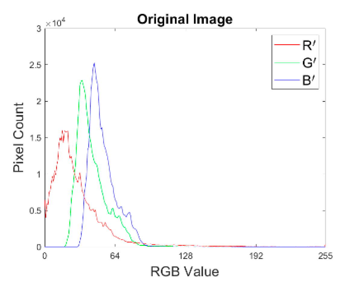
1. Separate image into its color channels R’, G’, and B’.

2. Build the filters for ψ Rm, ψ Gm, and ψ Bm.

$\begin{array}{l}{\psi }_{m,1}^{}=\left[0,1\right]{(\mathrm{B}}_m{-\mathrm{G}}_m^{})\\ {\psi }_{m,2}=\left[0,1\right]{(\mathrm{R}}_m{-\mathrm{G}}_m)\\ {\psi }_{m,3}^{}=\left[0,1\right]{(\mathrm{R}}_m{-\mathrm{B}}_m)\\ {\psi }_{m,4}^{}=\left[0,1\right]{(\mathrm{G}}_m{-\mathrm{B}}_m)\\ {\psi }_{m,5}^{}=\left[0,1\right]{(\mathrm{G}}_m{-\mathrm{R}}_m)\\ {\psi }_{m,6}^{}=\left[0,1\right]{(\mathrm{B}}_m{-\mathrm{R}}_m)\end{array}$

3. Set the [0, 1] state conditions for ψm,1, ψm,2, ψm,3, ψm,4, ψm,5, and ψm,6.

4. Use the ISED equation and set constant n to obtain Ln levels of decomposition, $\begin{array}{l}{R}_{m,n}^{}=R\prime -\frac{1}{\sqrt{2}}({\psi }_{m,1}^{}+{\psi }_{m,2}^{}+{\psi }_{m,3}^{}+{\psi }_{m,4}^{}+{\psi }_{m,5}^{}+{\psi }_{m,6}^{})\\ G_{m,n}^{}=G\prime -\frac{1}{\sqrt{2}}({\psi }_{m,1}^{}+{\psi }_{m,2}^{}+{\psi }_{m,3}^{}+{\psi }_{m,4}^{}+{\psi }_{m,5}^{}+{\psi }_{m,6}^{})\\ B_{m,n}^{}=B\prime -\frac{1}{\sqrt{2}}({\psi }_{m,1}^{}+{\psi }_{m,2}^{}+{\psi }_{m,3}^{}+{\psi }_{m,4}^{}+{\psi }_{m,5}^{}+{\psi }_{m,6}^{})\end{array}$

The equation forms the modified Rm,n, Gm,n, and Bm,n color channels.

5. Recombine the color channels to form a newly generated ISED image, (RGB)m,n.

6. Output the images for each Ln such that

${(RGB)}_{m,n}^{}=(RGB)\prime -\frac{1}{\sqrt{2}}{\displaystyle \sum _{n=1}^6\left({\psi }_{1,n}^{}+\dots +{\psi }_{m,n}^{}\right)}$.

7. Subtract the ISED image from the original image (RGB)’ to obtain the ISED filter image (7) $S_{m,n}^{-}\mathrm{for}\mathrm{n}=1~62\mathrm{and}\mathrm{m}=1~6$ for six levels of decomposition. This will generate 63 filters and the zero-state filter, which is a black image.

8. Reprocess the ISED output images (RGB)m,n following steps 2~8. When the desired decomposition level is achieved, end. Alternatively, one could code the entire formula; however, L6 would require 36 ensemble matrices for every color channel, so you would be processing 108 matrices to form an image.

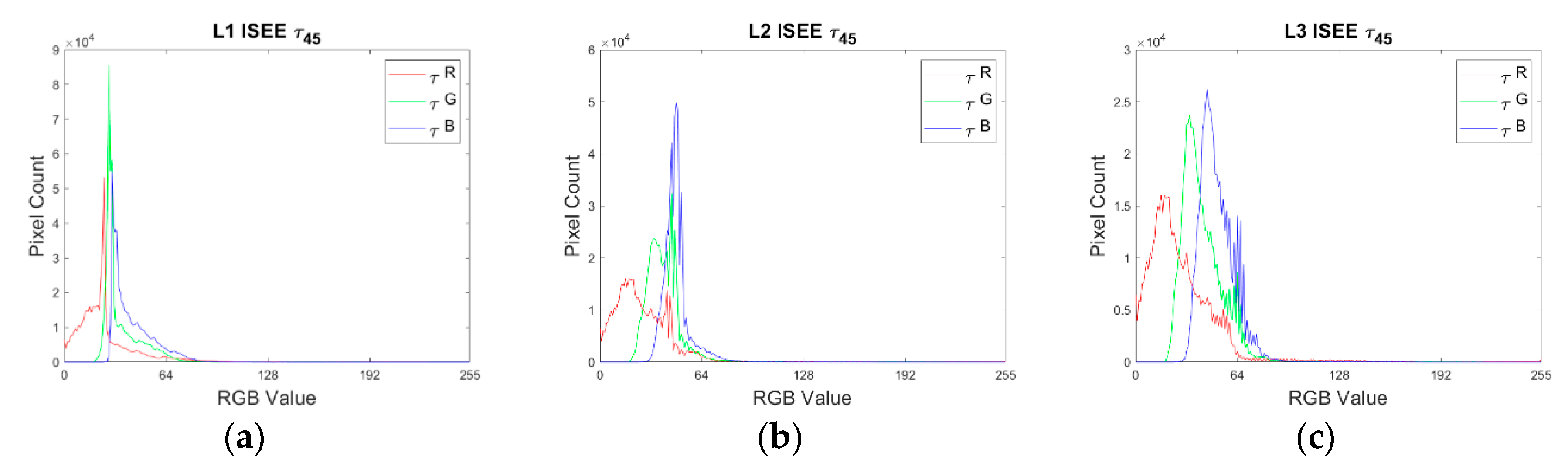
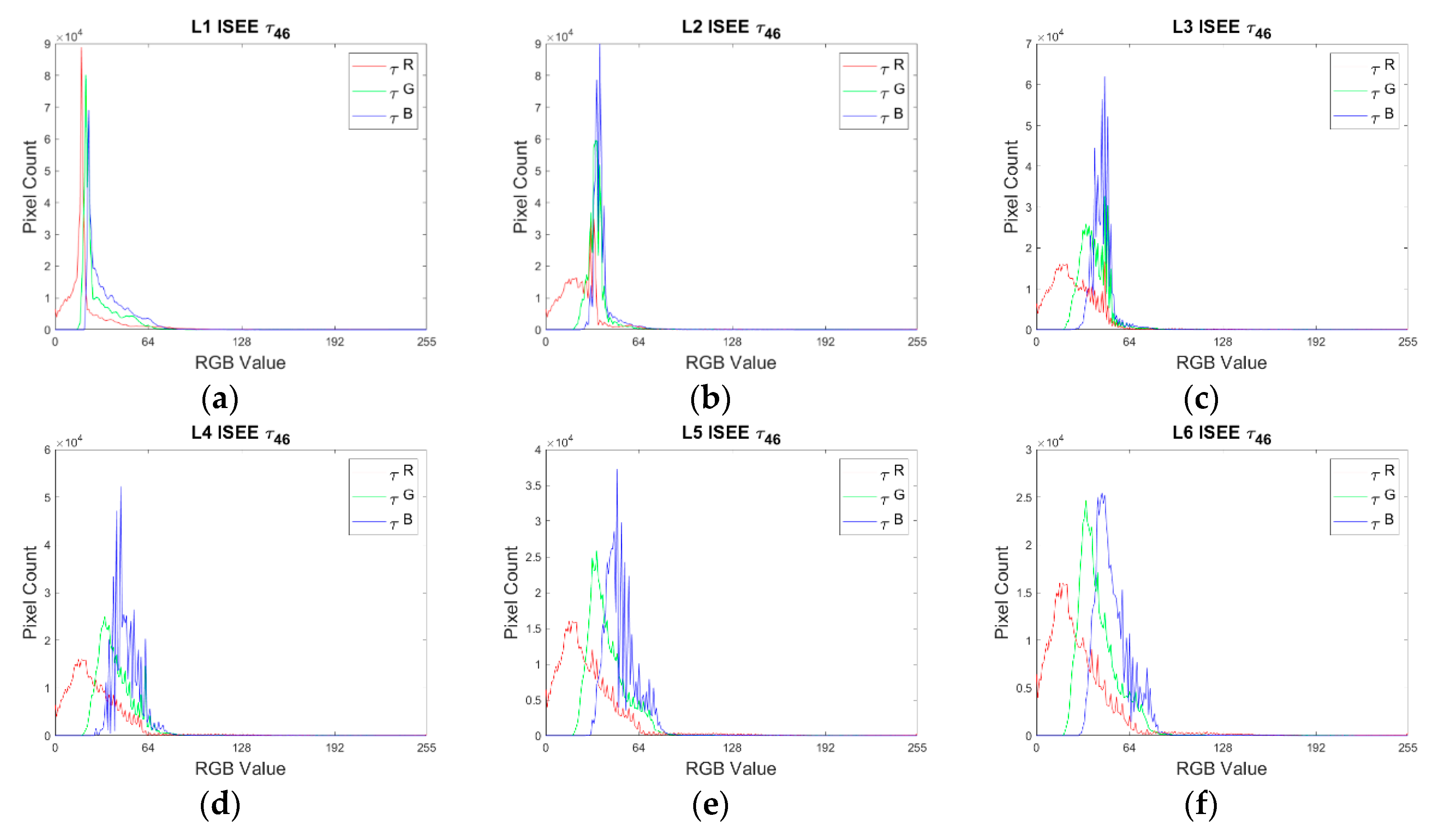
9. Combine the 63rd state ISED image (Sm,63) to each corresponding decomposition level with the Ln equivalent filter S−m,n such that $S_{m,63}^{}+S_{m,n}^{-},\mathrm{where}\mathrm{n}=1~62\mathrm{and}\mathrm{m}=1~6$ to produce the ISEE image τm,n. ${\tau }_{m,n}^{}=S_{m,63}^{}+S_{m,n}^{-}$.

By using Algorithm 1, there were 372 ISEE images that were generated. Full-reference and no-reference quality metrics were assessed to determine the properties of each of the generated deep Ln ISEE images. These images were then compared to past ISED results to determine if there was an overall improvement in the full-reference quality metrics. This will be discussed in detail in the Results and Discussion section.

4. Results and Discussion

The research objectives with deep Ln ISED and ISEE were to develop a new method of image processing that can selectively remove artifacts, types of glare, various distortions of an image, extract features, and simultaneously enhance contrast and features of an image. It was not a simple task; however, after extensively studying the most common image processing techniques, we believed that we could fill the image processing gap of knowledge by providing these useful techniques. Basic quantum mechanics played a key role in formulating Theorem 1 and the resulting ISED and ISEE equations. Deep Ln ISED and ISEE can filter out some of the unwanted effects and, as a byproduct, enhance others. In this section, we shall demonstrate the results of this study.

In the proposed ISEE research, Algorithm 1 was performed on a postprocessed SST image inset. The chromatically ordered image was obtained from NASA/JPL-Caltech/IPAC [18], and a crop of the M87 image was taken from an 11.1MB Tagged Image Format (TIF) file, “ssc2019-05b.tif”, available online at [19]. The image file had a resolution of 3580 × 3580 pixels prior to being cropped. The cropped test image was 322KB in size and had a resolution of 730 × 733 pixels. GIMP 2.10.14 was used to crop the image and it was saved as a lossless Portable Network Graphics file (PNG). Another tighter crop was taken to more clearly see the structures in the vicinity of M87′s IR core. The second crop had a resolution of 104 × 104 pixels, and the file size was 7.33 KB. The nominal values of the red, green, and blue channels were mapped from the infrared radiation wavelengths of 8.0, 4.5, and 3.5 μm, respectively [18]. The overlay images in Appendix A were constructed from combinations of different L6 ISEE images from the larger crop and a second L6 ISEE-generated image taken from the HST. The original HST TIFF file, “heic0815f.tif”, had a resolution 3854 × 3815, was 20.8 MB, and can be found online at [19]. The nominal values of the red, green, and blue channels were mapped from visible and infrared radiation wavelengths of 475, 606, and 814 nm, respectively [19]. The hardware configuration consisted of a standard gaming laptop with an Intel i7-8750H processor, 32 GB of RAM, and an NVidia GeForce GTX 1060 graphics processing unit. Matlab 2019a and Matlab 2020a were used to implement the algorithms.

In general, the information contained in the ISED image is shifted to the ISED filter as the levels of decomposition increase. Figure 1a is the original cropped image of the postprocessed insert taken from the SST [18]. Figure 1b is the first level of decomposition S_1,63, created in the previous study of ISED decomposition [1]. Figure 1c is the L2 ISED image of S_2,63. Figure 1d is the L3 ISED image of S_3,63 and Figure 1e–g are the deep L4, L5, and L6 ISED images S_4,63, S_5,63, and S_6,63, respectively. The images in Figure 1b–g are used in the creation of the proposed ISEE image reconstruction (S_m,63 images for Ln). I will reiterate that this ensemble state configuration was chosen for reconstruction; the reason is that the 63rd state ISED filter for all Ln has the maximum information removed from the image than all other states to avoid overlapping image data. This happens to be fortuitous because as Ln increases, the ISED filter (S⁻_m,n) information increases proportionally. One must first process deep Ln ISED images and filters in order to obtain ISEE images.

The cropped overlay image, Figure 2 plays a key role in the physical analysis for select deep Ln ISED and ISEE reconstrctions. This analysis will be covered in greater detail in the Conclusion. For the images in Figure 3a–l, you have both Ln ISED and ISEE reconstructions. The Ln ISED images are on the left side, and the corresponding Ln ISEE reconstructions are on the right. Some interesting features stand out in this set of images. First, the Ln ISED images for S_m,30 m = 1~6 remove the blues and the reds as the Ln increases. S_6,30 retains the edges of the outer IR dust ring, the IR core, and the IR shockwave structures that are produced by the superluminal jets. The counter-jet channel to the west of the IR core becomes visible. The vortex and the outburst can also be seen in the dusty core in S_6,30. Additionally, the counter-jet channel seems to be bent approximately 5° with respect to the left shockwave. This was verified with the HST/SST image overlay in Figure 2, where the SST ISEE generated image τ_6,30 and the HST generated ISEE image τ_6,19 in Figure A1b. The overlay was built in Gimp, and the top layer is the SST image with an 80% opacity. It was also rotated and cropped and saved in the PNG file format. The overlay selection of SST image τ_6,30 and HST image τ_6,19 was chosen because the SST image has the highest SSIM for τ_m,30 and the HST image isolated previously unseen wispy features surrounding the core. This was useful in aligning the image and revealing hidden features in the SST image.

The IQA metrics displayed in

Table 3. Average values for image quality assessments (IQAs) for τ_m,30 and S_m,30.

τm,n Sm,n	Image Quality Assessment Metrics ISEE
	SSIM	PSNR	MSE	NIQE	BRISQUE	PIQE
Original Image	1.00	NA	NA	8.22	43.38	100
τ1,30	0.63	22.04	406.91	6.84	41.58	44.43
τ2,30	0.57	21.27	485.76	7.16	42.82	63.76
τ3,30	0.68	22.85	337.25	6.97	45.08	63.73
τ4,30	0.76	24.44	233.89	7.15	41.61	59.49
τ5,30	0.81	25.71	233.89	6.89	52.78	58.98
τ6,30	0.84	26.68	139.81	6.96	61.80	54.90
S1,30	0.87	22.54	362.31	6.31	46.41	48.14
S2,30	0.62	19.02	814.23	6.92	36.99	48.51
S3,30	0.43	17.54	1146.2	7.25	45.11	43.21
S4,30	0.31	16.71	1388.4	7.32	46.14	44.13
S5,30	0.24	16.20	1558.3	7.81	46.45	47.82
S6,30	0.20	15.89	1674.4	8.05	46.56	48.46

for SSIM, PSNR, and MSE, (Defined in

Table 4. Image quality assessment techniques [20,21].

Quality Assessment	Definition
Structural Similarity Index (SSIM)	$SSIM(x,y)=\frac{(2{\mu }_x{\mu }_y+C_1)(2{\sigma }_{xy}+C_2)}{({\mu }_x^2+{\mu }_y^2+C_1)({\sigma }_x^2+{\sigma }_y^2+C_2)}$ for the images x,y: μx, μy, σx,σy, and σxy are the local means, standard deviations, and cross-covariance. C1 = (K1L)2, where k‹‹1 is a small constant and L is the dynamic range for the pixel values. Likewise, C2 = (K2L)2, where k‹‹1 is a small constant and L is the dynamic range for the pixel values, when α = β = γ = 1.
Peak Signal to Noise Ratio (PSNR)	$\begin{array}{l}PSNR=10lo{g}_{10}\hfill \end{array}\left(\frac{Ma{x}_f^2}{MSE}\right)$ where $Ma{x}_f^2$ is the maximum frequency squared
Mean Squared Error (MSE)	$MSE=\frac{1}{MN}{\displaystyle \sum _{X=0}^{M-1}{\displaystyle \sum _{y=0}^{N-1}{[I_1(i,j)-I_2(i,j)]}^2}}$

) NIQE, BRISQUE, and PIQE are well understood and are often employed as a standard in image analysis.

The SSIM produces a maximum score of one based on the images’ comparative contrast, local structure, and luminescence [20]. The PSNR indicates the peak error of the image and is used to determine compression loss in images and video [22]. Higher PSNR scores are better when compared to images that have gone through a similar process. Therefore, a rough comparison can be drawn between the same state images for varied Ln. Likewise, the MSE is also a good indicator to see the behavior of ISEE for deeper Ln as a comparative trend as a predictor for Ln > 6. Lower MSE scores are better. The NIQE is trained from a database of pristine images and various images with Gaussian distortions, so it can measure arbitrary distortions in the test images; lower scores are better [23]. Additionally, BRISQUE is trained from a database of known image distortions [24,25], while PIQE evaluates the local variance to detect block-wise distortion in order to calculate the quality of an image, where lower scores are better [26,27].

Table 5. Perception-based Image Quality Evaluator (PIQE) assessment range [27].

Quality Scale	Excellent	Good	Fair	Poor	Bad
Score range	[0, 20]	[21, 35]	[36, 50]	[51, 80]	[81, 100]

is for the assessment of PIQE scores, as recommended by [27]. From Table 5, it is clear as a trend, the SSIM increases apart from the L2 image. From our previous study, the ISED image seen in Figure 3a had an SSIM of 0.87. This is close to the value of the ISEE L6 image τ_6,30 SSIM of 0.84. The PNSR and MSE have both improved, so it is a probable indicator that the ISEE image has less noise. The NIQE is quite close, with S_1,30 equal to 6.31 and τ_6,30 equal to 6.96. The L6 BRISQUE score for the ISEE reconstruction has not improved over that of the ISED image S_1,30. The PIQE L6 is fairly close, but for the assessment range, S_1,30 falls into the fair category with a score of 48.14, while τ_6,30 is 54.9 in the poor category. The original photo PIQE was 100 and is in the bad category for the PIQE assessment range. For the higher SSIM ISED images, the ISEE images of L1 have better scores for the no-reference quality metrics and lower scores for the full-reference quality metrics. For deep Ln for ISED images S_m,30, there is a decrease in SSIM, PSNR, and MSE.

The L1 ISEE image τ_1,44 in Figure 4b has a well-defined outer IR dust ring, and the IR core is pronounced. The shockwaves and surrounding dust structures have good contrast against the black backdrop, where most of the blue channel information has been eliminated except the blue-biased glare portion of the image. Therefore, the image looks a bit blurred. As Ln increases, this blurring effect is reduced as the S⁻_m,44 information shifts. From the ISED image in Figure 4k, one can discern that there are two prominent features in the IR core of the S_6,44 image. The northwest image is the outburst that originates from the environs of the black hole in M87 and HST-1. The other feature relates to the vortex structure that coincides with the location of the black hole. In Figure 4l, L6 ISEE image τ_6,44, there is an interesting horizontal band structure that is perpendicular to the C-like shockwave on the western side of the image. This is either an artifact of the image or some mechanism that causes the appearance of planer shockwaves. This C-like structure is produced by a superluminal counter-jet that is traveling toward us and is not directly observable due to relativistic beaming [28].

The ISEE images in Figure 4 are constructed from an ISED filter (S⁻_m,44) with sparse information in L1. Then, as the decomposition progresses for deeper Ln, the information in the filter increases. Conversely, there is a lowering in SSIM for the ISED filter. This attributes to the trend of higher SSIM and PSNR for the ISEE reconstructions for τ_m,44, displayed in

Table 6. Average values for IQAs for τ_m,44 and S_m,44.

τm,n Sm,n	Image Quality Assessment Metrics ISEE
	SSIM	PSNR	MSE	NIQE	BRISQUE	PIQE
Original	1.00	NA	NA	8.22	43.38	100
τ1,44	0.51	20.33	603.14	5.91	37.37	43.54
τ2,44	0.38	19.34	757.28	5.97	42.52	68.82
τ3,44	0.49	20.61	564.73	6.08	42.16	72.28
τ4,44	0.64	22.46	369.28	6.50	42.10	68.71
τ5,44	0.76	24.50	369.28	6.73	41.59	63.23
τ6,44	0.84	26.58	143.08	6.86	35.31	61.16
S1,44	0.96	26.09	160.06	8.83	40.25	48.20
S2,44	0.83	21.22	491.38	7.71	37.49	47.52
S3,44	0.65	19.26	771.13	7.52	41.50	52.59
S4,44	0.45	17.80	1079.7	7.08	42.20	51.09
S5,44	0.29	16.74	1376.2	7.42	35.33	50.17
S6,44	0.18	16.04	1619.4	8.08	43.67	48.36

. Likewise, the MSE decreases for the most part, where L2 values for this filter seems to oscillate towards convergence to the test images as Ln increases.

By this point, it becomes apparent that the ISEE images vary in detail for Ln and there is an evolution of features one can gather from each generated image as reconstruction deepens. The images begin to converge to the original image while highlighting structures and changing as the process continues. When comparing the Ln ISEE and the ISEE images to the original image, a new world of information emerges from a single image. The implications of these processes for all branches of science that deal with image processing and feature extraction are broad. In Figure 5l, the vortex structure and the outburst structure are apparent in the IR dusty core.

From

Table 7. Average values for IQAs for τ_m,45 and S_m,45.

τm,n Sm,n	Image Quality Assessment Metrics ISEE
	SSIM	PSNR	MSE	NIQE	BRISQUE	PIQE
Original	1.00	NA	NA	8.22	43.38	100
τ1,45	0.92	28.26	97.11	6.71	46.13	50.33
τ2,45	0.93	30.15	62.84	6.43	54.96	57.25
τ3,45	0.97	34.06	25.54	7.01	62.45	40.25
τ4,45	0.98	36.46	14.70	7.60	59.25	52.23
τ5,45	0.99	38.05	14.70	8.07	55.69	50.64
τ6,45	0.99	39.50	7.30	7.94	54.92	50.47
S1,45	0.56	19.96	656.14	7.33	40.06	45.55
S2,45	0.15	16.08	1603.2	7.31	47.64	36.16
S3,45	0.05	15.16	1982.0	8.54	44.98	34.63
S4,45	0.02	14.90	2104.5	10.43	44.51	45.39
S5,45	0.01	14.80	2154.5	10.90	44.53	56.62
S6,45	0.01	14.74	2181.9	11.33	44.57	71.89

, it is apparent that the Ln ISED images quickly lose SSIM in this set of test images. The PNSR is low, and the MSE is high. The no-reference quality metrics also degrade. For the ISEE reconstruction, however, the SSIM is quite high and approaching that of the original image, and the PSNR and MSE improve as Ln increases. ISED and ISEE images are shown below Figure 6.

In the structure in Figure 7l on the dusty outer ring, there appears to be a globular mass that is in part feeding the black hole, but as it turns out when examining the overlay of the SST/HST image in Figure 2, there are dusty wisp-like structures, probably from a past ejection from the black hole, that appear to be pushing this matter outward like a bulldozer pushes dirt. So, as it is not feeding on the globular mass, it is most likely ejecting matter and energy particles.

According to

Table 8. Average values for IQAs for τ_m,46 and S_m,46.

τm,n Sm,n	Image Quality Assessment Metrics ISEE
	SSIM	PSNR	MSE	NIQE	BRISQUE	PIQE
Original	1.00	NA	NA	8.22	43.38	100
τ1,46	0.79	24.61	224.98	6.52	40.80	55.89
τ2,46	0.80	25.36	189.31	6.12	50.05	64.15
τ3,46	0.90	28.72	87.28	6.10	58.08	59.18
τ4,46	0.95	31.75	43.42	6.62	60.72	57.87
τ5,46	0.98	33.80	43.42	7.44	57.31	54.14
τ6,46	0.98	35.42	18.67	7.79	56.83	51.95
S1,46	0.74	21.93	417.37	7.36	45.55	44.38
S2,46	0.33	17.39	1185.7	6.55	45.62	44.64
S3,46	0.14	15.89	1675.0	7.23	47.30	38.58
S4,46	0.06	15.26	1938.5	8.41	45.25	38.62
S5,46	0.03	14.98	2060.8	10.59	44.64	39.95
S6,46	0.02	14.85	2129.0	11.34	44.54	52.44

, the SSIM and PNSR increase for ISEE τ_m,46 as Ln increases. The MSE decreases and NIQE shows improved quality over that of the original image and the ISED images S_m,46. The PIQE scores are, for the most part, better than the ISEE reconstruction because of the decomposition’s removal of the blue-biased glare. The glare is reintroduced in the reconstruction; however, the PIQE for the Ln ISEE images still displays improvement over that of the original image.

The ISEE images for τ_m,47 have the highest SSIM and PSNR out of all the presented images. Figure 7l has the closest SSIM to that of the original image. The color range that it isolates has the properties to isolate the vortex, outburst, globular structures, and boundary regions for the shockwaves. τ_6,47 is applied to the overlay of the HST image in Figure A1a–c.

The decompositional images of S_m,47 displayed in

Table 9. Average values for IQAs for τ_m,47 and S_m,47.

τm,n Sm,n	Image Quality Assessment Metrics ISEE
	SSIM	PSNR	MSE	NIQE	BRISQUE	PIQE
Original	1.00	NA	NA	8.22	43.38	100
τ1,47	0.99	32.95	32.98	7.70	43.39	23.34
τ2,47	0.98	33.60	189.31	7.93	44.33	29.95
τ3,47	0.99	35.43	18.63	7.79	46.20	43.30
τ4,47	0.99	36.97	13.07	7.94	49.00	50.40
τ5,47	0.99	38.32	13.07	8.01	51.38	53.60
τ6,47	0.99	39.73	6.91	8.06	51.87	51.48
S1,47	0.32	17.95	1041.30	6.75	45.44	44.96
S2,47	0.07	15.45	1855.0	7.77	45.32	34.54
S3,47	0.03	15.01	2049.4	9.69	44.51	44.10
S4,47	0.02	14.87	2120.9	10.41	44.49	47.82
S5,47	0.01	14.79	2160.3	10.89	44.53	61.77
S6,47	0.01	14.74	2185.0	11.32	44.57	71.62

also show a steep drop off in SSIM and PSNR as Ln increases and a rapid rise in MSE. The NIQE and PIQE increase, while the BRISQUE exhibits little variation. On the other hand, the Ln ISEE reconstructions have high SSIM, improved PNSR, and low IMSE. τ_6,47 has an MSE of 6.91 with an SSIM approaching 1. The NIQE and PIQE are also improved over that of the original image.

Sobel operator uses two 3 × 3 kernels that are convolved with the image (A). They are given by the following equations [3].

$$G_x=\left[\begin{array}{ccc}1& 0& -1\\ 2& 0& -2\\ 1& 0& -1\end{array}\right]\ast A{\mathrm{and}\mathrm{G}}_y=\left[\begin{array}{ccc}1& 2& 1\\ 0& 0& 0\\ -1& -2& -1\end{array}\right]\ast A$$

(10)

The gradient magnitude is defined to be

$$G=\sqrt{G_x^2+G_y^2}$$

(11)

for edge detection. This additional analysis was performed to attempt to determine more details on the physical structure near the dusty IR core and the IR ring.

Figure 8a displays a tighter crop of the original inset image in order to more clearly see the region of interest. Figure 8b is the gradient magnitude of the image that presents the edge features of the image. In the center of the image, the dark ring is where HST-1 is located. The actual galactic center and black hole lie on the inner ring to the west of the dark center. It is not apparent in this image, but it can be clearly seen in the overlay image in Appendix A, Figure A2a–c. Figure 8c is the x-gradient image and Figure 8d is the y-gradient image.

The image in Figure 9a is the tighter crop of the image seen in Figure 3l. τ_6,30 has the feature of the western counter-jet channel that is related to the C-like shockwave structure, which is produced by slowing heated dust from the superluminal jet. The image in Figure 3l is combined with the HST image in Figure A1b to produce the overlays presented in Figure A3a,b. The gradient magnitude image in Figure 9b displays a decent outline of the outer IR dust ring and the IR core. Figure 9c,d are τ_6,30′s x and y-gradient images.

The L6 ISEE image in Figure 10a has a higher SSIM than the other displayed images. This image is the tighter crop of Figure 7l. Figure 7l and Figure A1b are combined to produce the overlays in Figure A2a–c. The vortex, outburst, and globular features are apparent from the images in Figure 10a–d.

Figure 11 is the tricolor histogram of the original inset test image so that you can see the response for each channel. For all of the following histogram cases, the order is from L1 to L6 ISEE images and shows that for each deeper Ln for the cases of τ_n,30, τ_n,44, τ_n,45, τ_n,46, and τ_n,30, the histograms begin to converge to that of the original image. As stated earlier, some images eventually converge, and some remain divergent. To see full convergence for some cases, you would have to go much deeper than an L6 ISEE image.

The histograms for L1~L6 ISEE images τ_n,30 begin to converge when looking at the trend of the histograms in Figure 12a–f. It is observed that the spiked color channels begin to redistribute, and the pixel count scale becomes closer to the same order of the original image. If this state is computed for deeper levels than L6, this image most likely will converge, with less jaggedness in the histogram as Ln increases. The idea of a fully convergent image means that if Ln is sufficiently large, the algorithm will eventually generate the original image. I suppose this process would be analogous to using Fourier analysis to produce a square wave with amplitude 1 from an infinite sum of sinusoidal waves. Divergent cases do not generate the original image for any Ln.

The τ_n,44 images in Figure 13a–f possibly may not converge. The shifting of the peaks indicates that it may be converging to the original image, but this ensemble condition is not conclusive from the above histograms.

For the τ_n,45 cases, the histograms in Figure 14a–f indicate that the image is evolving into what we call a convergent case. This is logical due to the increased SSIM, PSNR, and improved MSE scoring as Ln increases. The ISED deep Ln image has a rapid decomposition; this causes more information to be contained in filter S⁻_m,n.

The ISEE reconstruction τ _n,46 is a movement towards convergence. If τ_n,46 is given enough Ln to evolve, it will replicate the original image. In Figure 15a–f, note the rapid evolution in the histograms that begin to evolve to the shape of the original test image’s histogram. This is an interesting feature of select deep Ln ensemble states for ISEE reconstructions.

The ISEE images produced from τ _n,47 are also convergent for deep Ln. The histogram in Figure 15f is associated with ISEE image τ_6,47. This image has the highest SSIM (.99), greatest PSNR (39.73), and the lowest MSE (6.91). The reconstruction has a narrow band of pixels that highlight the vortex, outburst, globular structures, and emphasizes regions in M87′s shock waves.The Histograms are shown below in Figure 16.

The CDF is presented in Figure 17a–f. The test images were separated into red, blue, and green color channels. Then the test images were compared for Ln 1~6 where R’, G’ and B’ is the CDF for the original image. CDF is shown to validate how ISEE evolves for Ln and to test for convergence. τ_m,30, τ_m,44, τ_m,45, τ_m,46, and τ_m,47 are represented by their corresponding lines in the legend. Figure 17f shows that τ_m,45, τ_m,46, and τ_m,47 are convergent for L6 and that it appears from the trends in Figure 17a–f that τ_m,30 will converge. It is also possible that τ_m,44 will converge as well, but at a deeper level than L6.

Table 10. Average values for IQAs.

States	Image Quality Assessment Metrics ISED
	SSIM	PSNR	MSE	NIQE	BRISQUE	PIQE
Original	1.00	NA	NA	8.22	43.38	100
Average ISED L1	0.70	22.8	473.1	7.22	42.90	46.23

is the average values for the image quality analysis conducted for 63 ISED-generated images from the previous study on the same M87 test image [1].

There were 62 ISEE images generated per Ln. Then, the averages were taken from the full-reference quality metrics and the no-reference quality metrics for each Ln. The results are above in

Table 11. Average values for IQAs for τ_m,n.

Average τm,n	Image Quality Assessment Metrics ISEE
	SSIM	PSNR	MSE	NIQE	BRISQUE	PIQE
ISEE L1	0.74	24.30	373.09	6.85	42.44	47.38
ISEE L2	0.69	24.35	492.33	6.78	47.25	55.25
ISEE L3	0.74	26.51	422.32	7.23	50.58	54.29
ISEE L4	0.79	28.31	370.96	7.66	50.86	54.21
ISEE L5	0.82	29.73	370.95	7.98	51.25	52.57
ISEE L6	0.83	30.87	319.63	8.06	51.41	53.29

. It is apparent that overall, the proposed method of deep Ln ISEE is an improvement for the full-reference quality metrics SSIM, PSNR, and MSE. The average NIQE is better than the average ISED L1 values for L1 and L2 ISEE reconstructions. L3 ISEE is on par with L1 ISED reconstructions. L4, L5, and L6 ISED NIQE are close to the average L1 ISED filters (the highest quality metrics of Ln overall). All average ISEE are better than that of the original M87 test image. The BRISQUE scores seem to be best for L1 ISEE, and from L2~L6, it appears to plateau around 51. The first level reconstruction on average scores is better than the original image. The PIQE scores are all better than the original image score of 100, which indicates poor quality. It stands to reason that the PIQE scores would be higher on average than the ISED filters due to the reconstruction process in ISEE.

5. Conclusions

Deep Ln ISEE is a promising tool for image processing. It can selectively filter via deep Ln ISED and generate many possible filters that can uncover features in a postprocessed image that was previously obscured due to biased glare, oversaturation, and color saturation. Then, with Ln ISEE, you can reconstruct and generate additional images that enhance image features of the generated images and improve full-reference quality metrics without substantial degradation of no-reference quality metrics. In many cases, the no-reference quality metrics were better than that of the original image for deep Ln ISEE images. The ISEE method opens many possibilities for future applications in image processing across the spectrum of scientific imaging. The ISEE reconstructed image is a type of narrowband filter, and the information is contained within the domain of the original image. ISEE filters, if given enough time to evolve to a very deep Ln, can result in the original image (converge) or diverge. ISED and ISEE both perform well, and for certain applications, ISED would be more suited then ISEE for contrast enhancement. In other instances, ISEE may be more desirable to extract finer detailed structures. It depends on the image you are trying to denoise or enhance and the types of features that you are trying to extract.

The specific application to observational astronomical imaging has revealed some profound insights by applying the novel ISEE method. Hidden within the postprocessed images from the HST and SST, we discovered an outburst that was located within the dusty IR core of M87 displayed in the overlay of Figure 2, which shows it directly relates to a dusty wisp-like structure (“purple right”) that seems to be emanating from HST-1. Hence, it is a localized distortion, most likely caused by the wisps. This structure appears to be slingshot around HST-1 and probably originates from the jet traveling through this structure. It stands to reason that the mass of HST-1 is strong enough to produce this slingshot effect by beam-splitting some of the superluminal jet particles to cause it to change its trajectory. Perhaps this and the jets’ interaction with matter in this region in part explains the outburst observed in HST-1. A second wisp-like structure (“purple left”) appears to follow a parallel path to that of HST-1. I suppose if HST-1 is massive enough, it would act like a beam collimator for the jets. This structure seems to emanate from the galactic core center of mass, which is offset from the black hole [29]. The path of the right jet is “right yellow”. The “orange circle” is the globular structure that is interacting with the jet. The “green U” is another structure that is being ejected from the galactic core from some type of explosive outburst. It appears to be pushing and heating the dust that forms the second globular structure, the “orange oval”. The channel for the counter-jet is displayed with the “left yellow line”. The suspected HST-2 is shown by the blue circle. HST-2 appears linear to the right counter-jet channel. The fact that the two jets are not aligned may be due to the angle in which this image is viewed. The counter-jet is firing in our direction, and the other jet is shooting away. This bending effect seems akin to a straw in a drinking glass half-filled with water. If you look at the glass, the straw appears bent. The viewing angle of the jets and the local effects of gravity in galaxy M87 may be warping space-time just enough to cause such an effect, or the gravitational effects of HST-2 are changing the angle of the counter-jet’s apparent trajectory by culminating the jet. The “blue lines” appear to be planar waves that seem to be parallel to the C-like shockwaves and perpendicular to the counter-jet channel. However, this effect could be a sampling error in the image. From the image, the apparent rotation of the black hole and the galaxies core is counterclockwise with respect to our viewing angle. Around the local vicinity core in Figure A3b, you can observe the detail of a swirling whirlpool structure, most likely caused by the rotation of the matter around the galactic core.

References

1. Tsai, D.Y.; Matsuyama, E.; Chen, H.M. Improving image quality in medical images using a combined method of undecimated wavelet transform and wavelet coefficient mapping. Int. J. Biomed. Imaging 2013. [Google Scholar] [CrossRef] [PubMed] [Green Version]
2. Taylor, T.R. Image State Ensemble Enhancement (ISEE). Available online: https://www.iseeimage.com (accessed on 4 June 2020).
3. Taylor, T.R.; Chao, C.-T.; Chiou, J.-S. Novel Image State Ensemble Decomposition Method for M87 Imaging. Appl. Sci. 2020, 10, 1535. [Google Scholar] [CrossRef] [Green Version]
4. Pratt, W.K. Digital Image Processing: PIKS Scientific Inside; John Wiley & Sons: Hoboken, NJ, USA, 2007. [Google Scholar]
5. Gonzalez, R.; Woods, R. Digital Image Processing, 2nd ed.; Prentice Hall: Upper Saddle River, NJ, USA, 2002; p. 793. [Google Scholar]
6. Gehrz, R.D.; Roellig, T.L.; Werner, M.W.; Fazio, G.G.; Houck, J.R.; Low, F.J.; Rieke, G.H.; Soifer, B.T.; Levine, D.A.; Romana, E.A. The NASA Spitzer Space Telescope. Rev. Sci. Instrum. 2007, 78, 011302. [Google Scholar] [CrossRef] [PubMed] [Green Version]
7. IRAC—Infrared Array Camera on the Spitzer Space Telescope. Available online: https://www.cfa.harvard.edu/irac/ (accessed on 4 June 2020).
8. Szajewska, A. Development of the Thermal Imaging Camera (TIC) Technology. Procedia Eng. 2017, 172, 1067–1072. [Google Scholar] [CrossRef]
9. Herman, C. The role of dynamic infrared imaging in melanoma diagnosis. Expert Rev. Dermatol. 2013, 8, 177–184. [Google Scholar] [CrossRef] [PubMed]
10. Kandlikar, S.G.; Perez-Raya, I.; Raghupathi, P.A.; Gonzalez-Hernandez, J.-L.; Dabydeen, D.; Medeiros, L.; Phatak, P. Infrared imaging technology for breast cancer detection—Current status, protocols and new directions. Int. J. Heat Mass Transf. 2017, 108, 2303–2320. [Google Scholar] [CrossRef]
11. Rajeesh, R.; Dwarakish, G. Satellite Oceanography—A review. Aquat. Procedia 2015, 4, 165–172. [Google Scholar] [CrossRef]
12. Thies, B.; Bendix, J. Satellite based remote sensing of weather and climate: Recent achievements and future perspectives. Meteorol. Appl. 2011, 18, 262–295. [Google Scholar] [CrossRef]
13. Vadivambal, R.; Jayas, D.S. Applications of Thermal Imaging in Agriculture and Food Industry—A Review. Food Bioprocess Technol. 2010, 4, 186–199. [Google Scholar] [CrossRef]
14. Rosique, F.; Navarro, P.J.; Fernández, C.; Padilla, A. A Systematic Review of Perception System and Simulators for Autonomous Vehicles Research. Sensors 2019, 19, 648. [Google Scholar] [CrossRef] [Green Version]
15. Harris, D.E.; Cheung, C.C.; Biretta, J.A.; Sparks, W.B.; Junor, W.; Perlman, E.S.; Wilson, A.S. The Outburst of HST-1 in the M87 Jet. Astrophys. J. 2006, 640, 211–218. [Google Scholar] [CrossRef]
16. Spitzer Captures Messier 87. Available online: https://www.jpl.nasa.gov/spaceimages/details.php?id=PIA23122 (accessed on 27 February 2020).
17. Peng, E.W.; Jordán, A.; Côté, P.; Takamiya, M.; West, M.J.; Blakeslee, J.P.; Chen, C.W.; Ferrarese, L.; Mei, S.; Tonry, J.L.; et al. The ACS Virgo Cluster Survey. XV. The Formation Efficiencies of Globular Clusters in Early-Type Galaxies: The Effects of Mass and Environment. Astrophys. J. 2008, 681, 197–224. [Google Scholar] [CrossRef] [Green Version]
18. Jet Propulsion Laboratory California Institute of Technology Spitzer Space Telescope. Available online: http://www.spitzer.caltech.edu/images/6592-ssc2019-05b-Spitzer-Captures-Messier-87-Jets- (accessed on 27 February 2020).
19. Lord of the Stars. Available online: https://www.spacetelescope.org/images/heic0815f/ (accessed on 4 June 2020).
20. Wang, Z.; Bovik, A.; Sheikh, H.; Simoncelli, E. Image Quality Assessment: From Error Visibility to Structural Similarity. IEEE Trans. Image Process. 2004, 13, 600–612. [Google Scholar] [CrossRef] [PubMed] [Green Version]
21. National Instruments Peak Signal-to-Noise Ratio as an Image Quality Metric. Available online: https://www.ni.com/en-us/innovations/white-papers/11/peak-signal-to-noise-ratio-as-an-image-quality-metric.html (accessed on 22 May 2020).
22. Huynh-Thu, Q.; Ghanbari, M. Scope of validity of PSNR in image/video quality assessment. Electron. Lett. 2008, 44, 800. [Google Scholar] [CrossRef]
23. Mittal, A.; Soundararajan, R.; Bovik, A. Making a Completely Blind Image Quality Analyzer. IEEE Signal Process. Lett. 2013, 22, 209–212. [Google Scholar] [CrossRef]
24. Mittal, A.; Moorthy, A.K.; Bovik, A.C. No-Reference Image Quality Assessment in the Spatial Domain. IEEE Trans. Image Process. 2012, 21, 4695–4708. [Google Scholar] [CrossRef]
25. Mittal, A.; Moorthy, A.K.; Bovik, A.C. Blind/Referenceless Image Spatial Quality Evaluator. In Proceedings of the 2011 Conference Record of the Forty Fifth Asilomar Conference on Signals, Systems and Computers (ASILOMAR), Pacific Grove, CA, USA, 6–9 November 2011. [Google Scholar] [CrossRef] [Green Version]
26. Venkatanath, N.; Praneeth, D.; Maruthi Chandrasekhar, B.; Sumohana, S.C.; Swarup, S.M. Blind image quality evaluation using perception based features. In Proceedings of the 2015 Twenty First National Conference on Communications (NCC), Bombay, India, 27 February–1 March 2015. [Google Scholar] [CrossRef] [Green Version]
27. Sheikh, H.; Wang, Z.; Cormack, L.; Bovik, A. LIVE Image Quality Assessment Database Release 2. Available online: https://live.ece.utexas.edu/research/quality (accessed on 28 November 2019).
28. Sparks, W.B.; Fraix-Burnet, D.; Macchetto, F.; Owen, F.N. A counterjet in the elliptical galaxy M87. Nature 1992, 355, 804–806. [Google Scholar] [CrossRef]
29. Batcheldor, D.; Robinson, A.; Axon, D.J.; Perlman, E.S.; Merritt, D. A Displaced Supermassive Black Hole in M87. Astrophys. J. 2010, 717. [Google Scholar] [CrossRef]
Figure 1. The original cropped inset image (a) and images of the Image State Ensemble Decomposition (ISED) decomposition levels (Lns) 1~6 Sm,63, where m = 1–6. ISED state 63 first level decomposition S1,63 (b). ISED images S2,63 (c), S3,63 (d), S4,63 (e), S5,63 (f), and S6,63 (g).
Applsci 10 03952 g001aApplsci 10 03952 g001b
Figure 2. Tight crop of Hubble Space Telescope (HST) τ6,19 and Spitzer Space Telescope (SST) τ6,44 overlay, 80% opacity with drawings.
Applsci 10 03952 g002
Figure 3. ISED and Image State Ensemble Enhancement (ISEE) Ln, n = 1~6 state 30 images. ISED image S1,30 (a), ISEE image τ1,30 (b), ISED image S1,30 (c), ISEE image τ2,30 (d), ISED image S3,30 (e), ISEE image τ3,30 (f), ISED image S4,30 (g), ISEE image τ4,30 (h), ISED image S5,30 (i), ISEE image τ5,30 (j), ISED image S6,30 (k), and ISEE image τ6,30 (l).
Applsci 10 03952 g003
Figure 4. ISED and ISEE Ln, n = 1~6 state 44 images. ISED image S1,44 (a), ISEE image τ1,44 (b), ISED image S1,44 (c), ISEE image τ2,44 (d), ISED image S3,44 (e), ISEE image τ3,44 (f), ISED image S4,44 (g), ISEE image τ4,44 (h), ISED image S5,44 (i), ISEE image τ5,44 (j), ISED image S6,44 (k), and ISEE image τ6,44 (l).
Applsci 10 03952 g004
Figure 5. ISED and ISEE Ln, n = 1~6 state 45 images. ISED image S1,45 (a), ISEE image τ1,45 (b), ISED image S2,45 (c), ISEE image τ2,45 (d), ISED image S3,45 (e), ISEE image τ3,45 (f), ISED image S4,45 (g), ISEE image τ4,45 (h), ISED image S5,45 (i), ISEE image τ5,45 (j), ISED image S6,45 (k), and ISEE image τ6,45 (l).
Applsci 10 03952 g005aApplsci 10 03952 g005b
Figure 6. ISED and ISEE Ln, n = 1~6 state 46 images. ISED image S1,46 (a), ISEE image τ1,46 (b), ISED image S2,46 (c), ISEE image τ2,46 (d), ISED image S3,46 (e), ISEE image τ3,46 (f), ISED image S4,46 (g), ISEE image τ4,46 (h), ISED image S5,46 (i), ISEE image τ5,46 (j), ISED image S6,46 (k), and ISEE image τ6,46 (l).
Applsci 10 03952 g006
Figure 7. ISED and ISEE Ln, n = 1~6 state 47 images. ISED image S1,47 (a), ISEE image τ1,47 (b), ISED image S2,47 (c), ISEE image τ2,47 (d), ISED image S3,47 (e), ISEE image τ3,47 (f), ISED image S4,47 (g), ISEE image τ4,47 (h), ISED image S5,47 (i), ISEE image τ5,47 (j), ISED image S6,47 (k), and ISEE image τ6,47 (l).
Applsci 10 03952 g007
Figure 8. Tight crop of m87 original image (a), gradient magnitude (b), directional gradient Gx Sobel (c), and the directional gradient Gy Sobel (d).
Applsci 10 03952 g008
Figure 9. Tight crop of m87 ISEE image τ6,30 (a), gradient magnitude (b), directional gradient Gx Sobel (c), and the directional gradient Gy Sobel (d).
Applsci 10 03952 g009
Figure 10. Tight crop of m87 ISEE image τ6,47 (a), gradient magnitude I*2 (b), directional gradient Gx Sobel (c), and the directional gradient Gy Sobel (d).
Applsci 10 03952 g010
Figure 11. Histogram of the M87 inset image.
Applsci 10 03952 g011
Figure 12. Histograms of ISEE images τ1,30 (a), τ2,30 (b) τ3,30 (c), τ4,30 (d), τ5,30 (e), and τ6,30 (f).
Applsci 10 03952 g012aApplsci 10 03952 g012b
Figure 13. Histograms of ISEE images τ1,44 (a), τ2,44 (b), τ3,44 (c), τ4,44 (d), τ5,44 (e), and τ6,44 (f).
Applsci 10 03952 g013
Figure 14. Histograms of ISEE images τ1,45 (a), τ2,45 (b), τ3,45 (c), τ4,45 (d), τ5,45 (e), and τ6,45 (f).
Applsci 10 03952 g014aApplsci 10 03952 g014b
Figure 15. Histograms of ISEE images τ1,46 (a), τ2,46 (b), τ3,46 (c), τ4,46 (d), τ5,46 (e), and τ6,46 (f).
Applsci 10 03952 g015
Figure 16. Histograms of ISEE images τ1,47 (a), τ2,47 (b), τ3,47 (c), τ4,47 (d), τ5,47 (e), and τ6,47 (f).
Applsci 10 03952 g016aApplsci 10 03952 g016b
Figure 17. Cumulative distribution function (CDF) of the original image and τm,n for each color channel. CDF of L1 (a), L2 (b), L3 (c), L4 (d), L5 (e), and L6 (f).
Applsci 10 03952 g017aApplsci 10 03952 g017b