High-Efficiency Simulation Framework to Analyze the Impact of Exhaust Air from COVID-19 Temporary Hospitals and its Typical Applications

Abstract

The outbreak of COVID-19 resulted in severe pressure on the existing medical infrastructure in China. Several Chinese cities began to construct temporary hospitals for the centralized treatment of COVID-19 patients. The harmful exhaust air from the outlets of these hospitals may have a significant adverse impact on the fresh-air intakes and surrounding environment. Owing to the need to rapidly construct these hospitals within 6–10 days, just a few hours are allowed for the analysis of the impact of this exhaust air on the environment. To overcome this difficulty, a high-efficiency simulation framework is proposed in this study. Based on the open-source computational fluid dynamics software, FDS, the proposed framework is adaptive and incorporates building information with different levels of detail during various design phases of the hospital, and has been applied in the design of the Wuhan Huoshenshan Hospital, the first typical COVID-19 temporary hospital in China. According to the simulation results, neither the fresh-air intakes nor the surrounding buildings would be polluted by the harmful air discharged from the air outlets of the Huoshenshan hospital. The proposed simulation framework can provide a reference for the design and overall planning of similar hospitals in China and other affected countries.

1. Introduction

The outbreak and spread of COVID-19 had affected many countries around the world by mid-March 2020. The cumulative confirmed cases across the world have exceeded 400,000, and this large number of patients has resulted in significant pressure on the existing medical infrastructure in several countries.

In response to the shortage of medical resources, some Chinese cities began to build temporary hospitals for the centralized treatment of patients suffering from pneumonia. For example, Wuhan constructed two new COVID-19 temporary hospitals, namely the Huoshenshan Hospital and Leishenshan Hospital; Beijing reconstructed the Xiaotangshan Hospital, which was used for the treatment of patients suffering from severe acute respiratory syndrome (SARS) in 2003. For the design of the heating, ventilation, and air conditioning (HVAC) system in these hospitals, negative air pressure and a special exhaust system must be utilized to discharge the harmful air emitted by patients. The harmful air needs to be exhausted at a higher altitude to prevent the virus from spreading to the unaffected areas of the hospital. Although the exhaust system is generally equipped with filtration devices, there is still a certain degree of risk associated with infections after the harmful air is discharged through the air outlets. According to the research on the infectivity of SARS, if the air exhaled by a SARS patient is not diluted to less than 10,000 times using clean air, it could result in a risk of infection [1]. Considering the limited knowledge on COVID-19 at present, if the ground reality of these hospitals can be considered in the simulation of the dispersion process of the exhaust air in an outdoor environment, the infection risk caused by the harmful air can thus be quantitatively evaluated, which will provide designers with a more specific reference during the design of such hospitals. Because the design and construction of the temporary hospital must be completed within 6–10 days, limited time is allocated for the simulation and analysis of the impact of exhaust air on the environment. Moreover, considering the extremely high infectivity of SARS-CoV-2, the design scheme of the air outlet and fresh-air intake for the temporary hospital needs to undergo multiple rounds of iteration and verification in a short time. Hence, the corresponding simulation method must meet the requirements of both high accuracy and efficiency.

Generally, four common methods can be used to study pollutant dispersion around buildings, including (1) field measurement, (2) physical modeling, (3) semi-empirical methods, and (4) numerical modeling [2]. The field measurement method can only be used to record the concentration of pollutants in the built-up area, which cannot provide a reference for the design of a temporary hospital. Physical modeling methods require fabricated scaled models of buildings and wind tunnel tests, which must meet the similarity criteria and are generally time-consuming and labor-intensive [3]. Thus, it is difficult for engineers to realize a rapid evaluation of the impact of exhaust air in the condition of an emergency response through the physical modeling method.

The commonly used semi-empirical methods include the Gaussian models and the American Society of Heating, Refrigerating and Air-Conditioning Engineers (ASHRAE) models, which are based on a Gaussian distribution of the plume in the vertical and horizontal directions under steady conditions [4,5]. These models usually require certain empirical or semi-empirical parameters from observations and make crude simplifications [6]. While these models are successfully employed for simplified flow configurations and meet the demands of high-efficiency simulations, they are only useful for landscapes that are approximately flat and unobstructed. Further studies are required if these models are to be used in cities and other built-up areas with complex surfaces [2].

In recent years, computational fluid dynamics (CFD) technology has been gradually applied to the study of pollutant dispersion around buildings. In terms of the scale of the analysis object, the configurations used in previous studies can be categorized into three typical cases: an isolated building, a single street canyon, and building complexes. Owing to the fact that the simulation of pollutant dispersion around building complexes generally calls for a higher number of computing resources, most of the related studies adopted the Reynolds-averaged Navier–Stokes equations (RANS) method [7,8,9,10,11,12], while the large eddy simulation (LES) method [13] was used in limited cases. By contrast, at the level of a single street canyon, both RANS [14,15,16] and the LES method [17,18,19] were widely used. Moreover, with respect to the level of an isolated building, except for the RANS [20,21,22,23] and LES method [24,25], the direct numerical simulation method was also adopted in published research [26].

Although there are many sophisticated methods to simulate pollutant dispersion around buildings, two challenges must be addressed when applying the abovementioned semi-empirical methods or numerical modeling methods to this study. (1) The temporary hospital generally consists of building complexes with several types of configurations, around which the pollutant dispersion cannot be simply simulated using semi-empirical methods. (2) On the one hand, considering the urgent construction needs of temporary hospitals, faced by many cities around the world, the purchase of commercial CFD software cannot meet the needs of an emergency response either in time or cost. On the other hand, certain common commercial CFD software, such as Fluent, consumes a significant number of computing resources and takes an extended time to complete the CFD computations [27]. Therefore, to help engineers complete the design of the temporary hospital quickly, open-source CFD software with high computing efficiency and easy operation is the need of the hour.

FDS (Fire Dynamic Simulator) is an open-source CFD software developed by the National Institute of Standards and Technology [28]. The software was initially developed for fire simulations. With the gradual enrichment of its functions, it has also been applied to pollutant dispersion simulations [29,30]. The advantages of the FDS software can be enumerated as follows: (1) the open-source feature of FDS dramatically simplifies the acquisition and installation process and facilitates the promotion of the software; (2) the LES method is inherently adopted by the FDS so that the transient characteristics of the flow field and pollutants can be captured; and (3) compared with commercial CFD software, it is convenient and straightforward for engineers to complete the mesh generation of the computational domain in the FDS so that the design scheme of the temporary hospital can be quickly evaluated. A trial application of the FDS for the pollutant dispersion simulations has been successfully performed by Gu et al. [31,32]. Owing to the above advantages, FDS is adopted for this study.

Aiming to help engineers swiftly finish the design of temporary hospitals, a high-efficiency simulation framework, based on FDS, to analyze the impact of harmful exhaust air is proposed in this study. It should be noted that during the design cycle of the temporary hospital, engineers may be faced with different analysis objects during different design phases. Specifically, in the initial design phase, the feasibility of the conceptual design scheme needs to be quickly evaluated through numerical simulations; in the transition phase, the design scheme of the air outlet and fresh-air intake needs to be simulated and evaluated to ensure that the harmful air, discharged from air outlets, does not pose a secondary infection risk to the fresh-air intakes; in the final phase, it is necessary to quantitatively assess the impact of the harmful exhaust air on the surrounding environment of the temporary hospital.

In the following sections, the proposed high-efficiency simulation framework is first introduced in detail. Subsequently, the accuracy and efficiency of the proposed simulation method are verified through a comparison with the results of both wind tunnel tests and simulations using Fluent. Finally, the case study of the Wuhan Huoshenshan Hospital is used to demonstrate that the proposed simulation framework is a practical method to assist designers in completing the HVAC design of temporary hospitals in a short time.

2. Proposed Simulation Framework

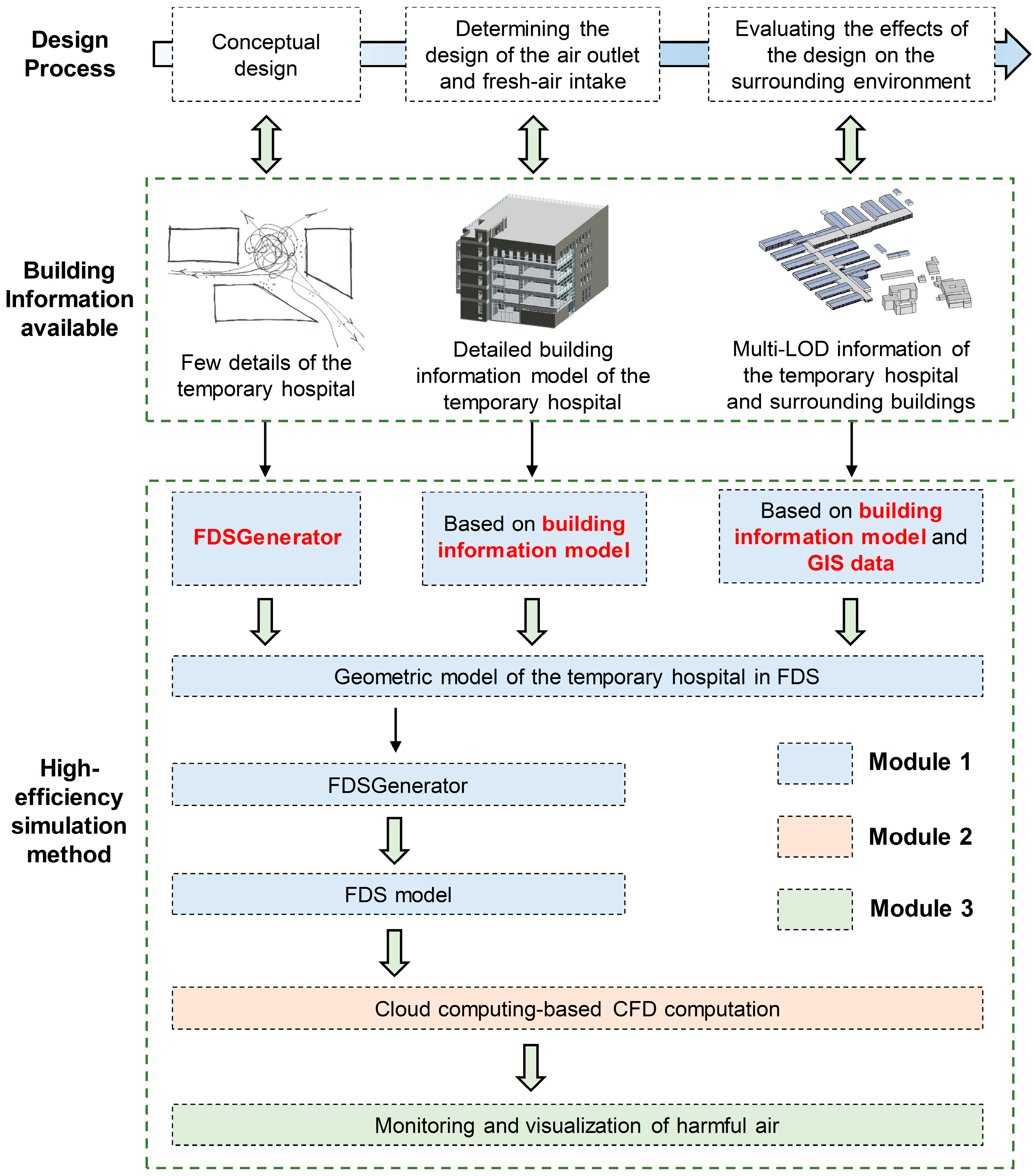
During the design cycle of COVID-19 temporary hospitals, the analysis objects in different design phases may present building information with different levels of detail (LODs). Specifically, in the initial phase, the analysis object is the conceptual design, which only contains low-LOD information relating to building configurations and sizes; in the transition phase, the analysis object is the temporary hospital with detailed design drawings or a building information model (BIM); and in the final phase, the analysis object is the overall built environment including the temporary hospital and surrounding buildings. It is worth noting that while detailed design drawings of the temporary hospital are available in the later design phase, it is challenging for engineers to collect the detailed drawings or BIMs of all surrounding buildings in a limited period given that the surrounding buildings may be constructed by different companies and may also include old buildings that may lack the requisite detailed drawings. The proposed high-efficiency simulation framework (see Figure 1) adapts to the building information with different LODs during various design phases of the temporary hospital.

The simulation framework is composed of three modules: (1) high-efficiency modeling of the temporary hospital, (2) cloud computing-based CFD computation, and (3) monitoring and visualization of the harmful air. In Module 1, the geometric model of the temporary hospital building is firstly constructed, after which detailed information of other objects (i.e., computational domain, air outlets, wind profile in the urban boundary layer (UBL), monitoring points and slices for recording the concentration of harmful air) that are required for the CFD simulation, is supplemented to build a complete FDS model. To handle building information with various LODs during the three design phases mentioned above, three high-efficiency modeling methods are proposed correspondingly and have been integrated into the specially-developed FDSGenerator program. In Module 2, the simulations and analyses of cases with various wind profiles and design schemes are completed based on cloud computing technology. In Module 3, the simulation results are visualized to help engineers evaluate design schemes in an improved manner.

2.1. Module 1: High-Efficiency Modeling of Temporary Hospitals

2.1.1. FDSGenerator Program

The FDS model can be constructed by means of command lines [33]. The commands commonly used in FDS, for the simulation of pollutant dispersion, are shown in

Table A1. Commands commonly used in FDS for the simulation of pollutant dispersion.

FDS Command	Function
&HEAD	To represent the beginning of the FDS file.
&TIME	To set the simulation time.
&WIND	To define the wind profile.
&VENT	To create a vent for the air outlet or define the boundary condition.
&MESH	For mesh generation.
&SPEC	To create a particle for representing the pollutant.
&DEVC	To create a monitoring point.
&PART	To classify objects in the model.
&SURF	To create a surface for the air outlet.
&OBST	To create a solid object.
&SLCF	To create a monitoring slice.
&TAIL	To represent the end of the FDS file.

in Appendix A. Owing to the fact that the quantitative assessment of the impact of harmful exhaust air on the environment generally has to be completed within a limited time, it is challenging for designers to master the modeling function of FDS in a short time. Therefore, based on Python and PyQt5 [34], an easy-to-use program named FDSGenerator was developed in this study to facilitate designers and enable them to quickly build FDS models. The graphical user interface (GUI) for this program is shown in Figure 2, and the main functions of the program can be categorized into three types: (1) input of model information; (2) mesh generation; and (3) reading, writing, and visualization.

(1)

Input of model information

This function allows users to input model information such as the parameters of the mean wind speed profile in the UBL, the vertex coordinates of the geometric model, the coordinate and ventilation volume of each air outlet, the concentration of harmful air in the exhaust air from each air outlet, and the locations of monitoring points and slices.

The ventilation volume, V_R, of each air outlet can be easily calculated based on the design drawings, and the concentration of harmful air in the exhaust air from each air outlet can be obtained through the following method. Generally, two patients share a ward in a COVID-19 temporary hospital. The average rate of breathing air from a seated person is reported to be between 0.27 and 0.33 m³/h, with significant variation due to physiological activity conditions [1]. In this study, the reference breathing rate, V_P, of a COVID-19 patient is assumed to be 0.30 m³/h. This value was also adopted by Jiang et al. [1] for the simulation of indoor SARS transmission. Thus, the total amount of harmful air exhausted by patients in N wards sharing one air outlet is 2V_P∙N. Considering the positive effect of the filtration devices installed at the air outlets, the mass ratio of harmful air in the exhaust air from one air outlet can be calculated through Equation (1):

$$R=2\beta N{V}_p/V_R,$$

(1)

where β is a coefficient reflecting the filtering capacity of the filtration device for harmful air.

(2)

Mesh generation

This feature allows users to design specific grid schemes, including a single-resolution grid and a multi-resolution grid.

(3)

Reading, writing, and visualization

The “reading” function enables users to read the pre-constructed building geometry model or the completed FDS model in the program, as well as other information required for the CFD simulation (i.e., coordinates and ventilation volumes of air outlets, and locations of monitoring points and slices) in pre-defined formats. The “writing” function allows users to generate the FDS model file based on the information entered, and output simulation results at monitoring points. The “visualization” feature enables users to observe the constructed objects (i.e., building shapes, as well as locations of air outlets and monitoring points) in a specific window on the right side of the GUI. Additionally, users can freely delete incorrect objects through this function.

Based on the FDSGenerator program, the corresponding high-efficiency modeling methods for different design phases are proposed and will be introduced in detail in the following sections.

2.1.2. Conceptual Design

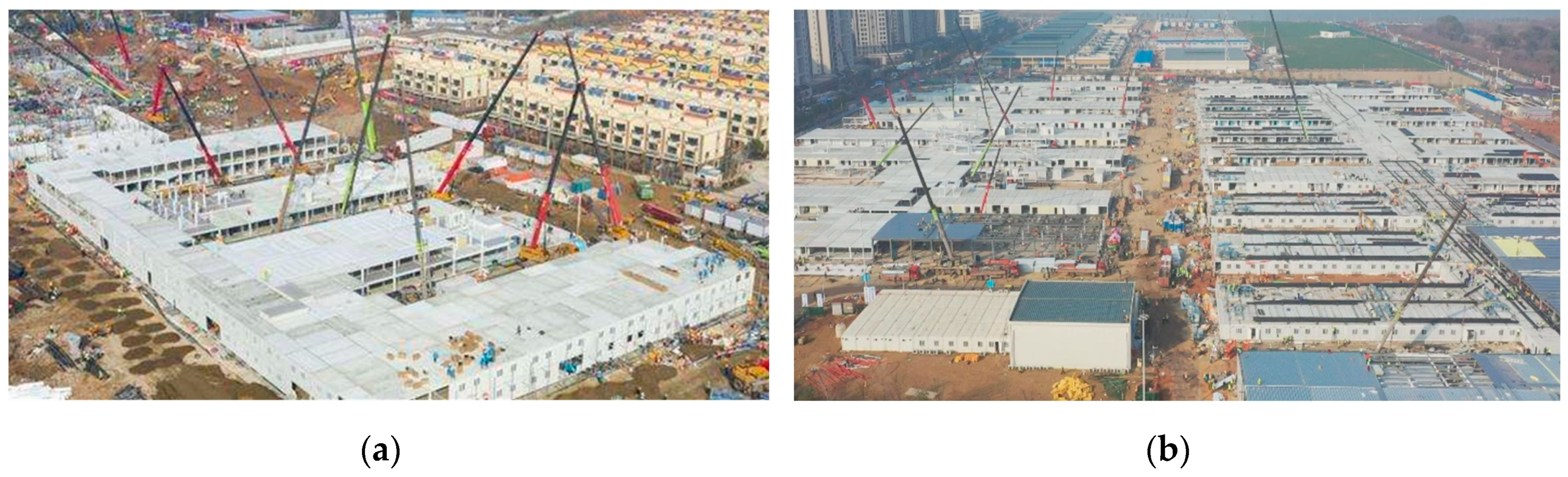
In the conceptual design phase, several features of the temporary hospital, such as the heights of air outlets and fresh-air intakes, need to be assessed and optimized. At this juncture of the design phase, given that the building shape is yet to be determined, it is feasible to use a simplified building geometry to help engineers better evaluate the pros and cons of different conceptual design schemes. It should be noted that FDS can only support a structured grid with a cuboid shape. Hence, the building model in FDS must be represented by cuboids. Furthermore, for buildings with complicated shapes, the building must be approximated by a large number of cuboids. Fortunately, since the COVID-19 temporary hospitals are mostly composed of box-type buildings with standard modules, their shapes are generally cuboid (see Figure 3). Therefore, the user can easily divide the geometric model of the conceptual design into multiple cuboids, after which the geometric model can rapidly be built, based on the vertex coordinates of these cuboids and the FDSGenerator program. Finally, the information relating to other objects required can easily be supplemented through the FDSGenerator to generate a complete FDS file required for the CFD computation.

2.1.3. Evaluating the Design Schemes of the Air Outlets and Fresh-Air Intakes

In this design phase, the detailed drawings and BIMs (e.g., SketchUp model, Revit model, or AutoCAD model) of the temporary hospital can generally be obtained from the corresponding design agency. Hence, the data transformation from the information model to an FDS model can be easily realized through Pyrosim [35] and the FDSGenerator program. Pyrosim is a popular pre-processing program for FDS. Figure 4 shows the detailed workflow of the data transformation. The information model developed in widely used 3D modeling computer programs (i.e., AutoCAD, SketchUp, and Revit) are first exported to an intermediate file (i.e., DWG, FBX, and DXF file correspondingly), which is then imported into Pyrosim to generate the FDS model that only retains the geometries of the building components. Subsequently, the FDS model generated by Pyrosim is imported into the FDSGenerator through the “reading” function mentioned above, and the other information required by the CFD simulation can easily be supplemented in the FDSGenerator. By employing Pyrosim and the developed FDSGenerator program, a complete model conversion, capable of containing all the geometrical and other relevant data, is achieved to transform the information model to an FDS model.

2.1.4. Evaluating the Impact of Exhausted Harmful Air from a Temporary Hospital on the Surrounding Environment

The impact of exhausted harmful air on the surrounding environment needs to be evaluated quantitatively before the design of the temporary hospital is completed. In this design phase, two challenges must be addressed if there exists a large number of old buildings in the target area. (1) Since the target area may have buildings designed by different companies and constructed over different years, it is challenging for engineers to collect detailed drawings or BIMs of all the surrounding buildings in a short time. In addition, it is highly possible that a few old buildings around the proposed temporary hospital lack detailed drawings, which introduces more challenges relating to the collection of building information. Thus, the modeling method introduced in Section 2.1.3 cannot be used directly to build the FDS model for the target area. (2) The surrounding buildings may have various complicated shapes, which cannot be easily modeled through the FDSGenerator program.

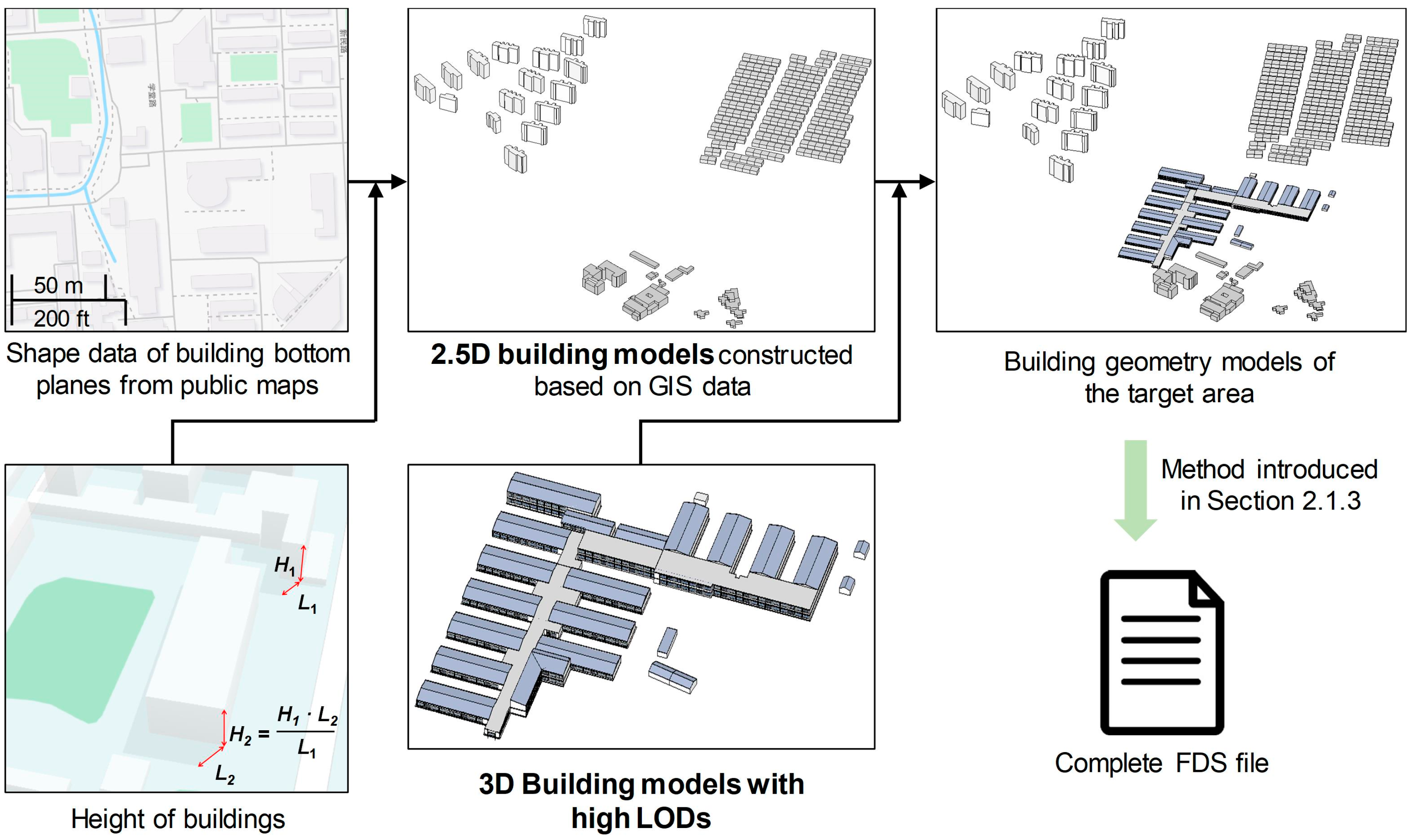
To overcome the abovementioned difficulties, a high-efficiency modeling method based on BIM and geographic information system (GIS) data for the FDS model of the target area is proposed. The workflow of this method is shown in Figure 5. Firstly, the shape file and corresponding plot scale of the buildings lacking drawings and BIMs can be easily obtained from public map sources (e.g., OpenStreetMap (https://www.openstreetmap.org), Google Maps (https://www.google.com/maps), and Baidu Maps (https://map.baidu.com)). Simultaneously, if we know the height, H₁, of a specific building near or in the target area, we can measure the shadow length, L₁, of this specific building and the shadow length, L_i, of any building in the target area using online maps such as Google Maps and Baidu Maps. Then the height of each building in the target area can be calculated through the following equation based on the similar triangle theory:

$$H_i=\frac{H_1\cdot L_i}{L_1},$$

(2)

It should be noted that two requirements should be met before calculating building height through the above method. The first one is that at least one vertical edge of the target building can be clearly seen for the observer on online maps. The other one is that building shadow should also be as clear and unambiguous as possible, so that the observer can accurately measure it with the length-acquisition tool on online maps. These two requirements can be easily met when modelling the COVID-19 temporary hospital and its surrounding buildings, given that the temporary hospital is usually built in an open area, not in the city center. Given the shape data of building bottom planes and the height data of each building in the target area, the 2.5D geometry models of the buildings lacking drawings and BIMs can be built quickly using 3D modeling software like SketchUp. Subsequently, the geometry model of the target area can be constructed by merging the 3D model of the temporary hospital and the 2.5D building models constructed using GIS data. Finally, the complete FDS file of the target area can be generated through the method introduced in Section 2.1.3.

2.2. Module 2: Cloud Computing-Based CFD Computation

The governing equations of the mathematical modelling of FDS solver can be found in McGrattan et al. [33]. It is worth noting that various parameters (e.g., wind direction, wind speed, building configuration, and heights of air outlets and fresh-air intakes, among others) need to be considered when performing CFD simulations. Although FDS is considered as software with high computation efficiency, a large number of simulation cases resulting from these various parameters will bring about enormous pressure on computing resources. Here, cloud computing resources can be utilized to address this challenge, given that the FDS is open-source software and can be installed on any number of computers. FDS supports parallel computing technologies for the Message Passing Interface (MPI) and Open Multi-processing (OpenMP), and can be run on both Windows and Linux operating systems. Hence, engineers can purchase multi-core computing units on cloud computing platforms (the cost is approximately 0.03–0.06 dollar per core hour in China) and freely adjust the number of purchased units according to the number of simulation cases to meet the needs of enormous computing resources that rise significantly in a short time.

2.3. Module 3: Monitoring and Visualization of Harmful Air

After the CFD computation based on cloud computing technology is completed, there are two ways in FDS to investigate the distribution and concentration of exhausted harmful air.

(1)

Through the recorded results at monitoring points

Provided that the FDS model is built through the proposed high-efficiency modeling method, several data files recording the simulation results at various monitoring points will be generated automatically after the CFD computation is successfully completed. These files provide engineers with time–history data relating to the concentration of exhausted harmful air at each pre-defined monitoring point, which can be further used for the analysis and evaluation of the design scheme.

(2)

Through the animation of tracer particles and isosurfaces

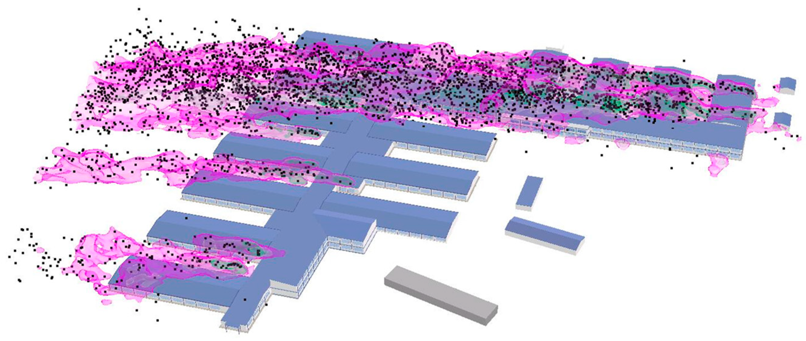
In FDS, the “tracer” function can be used to monitor the trajectories of particles that represent the harmful dispersive air, and the “&ISOF” command can be used to generate several isosurfaces with different concentration values. Once the CFD computation is successfully completed, engineers can investigate the animations of the pre-defined tracer particles and isosurfaces in SmokeView [28], an open-source post-processing program for FDS. One typical frame of a representative animation is shown in Figure 6, where the black particles represent the exhausted harmful air dispersing in the air while the pink curved surfaces represent the isosurfaces with a particular concentration value.

3. Efficiency and Accuracy of the Proposed Simulation Method

In this study, both the proposed FDS-based simulation method and the widely used commercial CFD software, Fluent, were adopted to simulate the dispersion of pollutants as performed by Li and Meroney [36]. A comparison of the modeling and computational efficiency of the two software indicates that the proposed simulation method is sufficiently efficient to satisfy the needs of the rapid design of the COVID-19 temporary hospitals. Moreover, the accuracy of the proposed method in the pollutant dispersion simulation for an individual building was verified through a comparison between the experimental results presented by Li and Meroney [36] and the simulation results.

Furthermore, to verify the accuracy of the proposed method in the pollutant dispersion simulation for a street canyon, the proposed FDS-based simulation method was adopted to simulate the dispersion of pollutants as performed by Tominaga and Stathopoulos [37].

3.1. Wind Tunnel Test Performed by Li and Meroney

Figure 7 shows the wind tunnel test performed by Li and Meroney [36]. The wind tunnel facility used in the experiment was a thermally stratified wind tunnel located at the Fluid Dynamics and Diffusion Laboratory at Colorado State University. In the wind tunnel, of the size of 1.0 m × 0.5 m × 0.5 m, a cube with a side length of 0.05 m was used to represent a separate building. A circular vent with a pollutant release rate of 12.5 cm³/s was set at the center of the rooftop. To record the concentration of the pollutant on the building surface, several monitoring points were set on the centerline of the top surface along the downwind direction and the centerline of the leeward surface along the vertical direction, which are shown as the red dashed lines in Figure 7.

3.1.1. FDS Model to Simulate the Experiment

The FDS model used to simulate the experiment can be easily constructed through the method introduced in Section 2.1.1 based on the FDSGenerator. The wind speed profile of the FDS model is made consistent with that used in the wind tunnel test (see Figure 8). The size of the computational domain in the FDS model was the same as that of the wind tunnel. A multi-grid technique, which refined the computational domain under the height of 0.1 m, was employed in the FDS model to improve the simulation’s accuracy. Specifically, the grid size of the domain under the height of 0.1 m was set to 0.0025 m × 0.0025 m × 0.0025 m. The grid size of the domain between the heights of 0.1 m and 0.3 m was set to 0.005 m, whereas that of the remaining domain was set to 0.02 m. The total number of cells was 3.255 × 10⁶. The constant pollutant release rate of the vent at the center of the cube rooftop was set to 1.25 × 10⁻⁵ m³/s according to the experiment setup, and the mass fraction of pollutant on the vent surface was taken as 100%. According to the FDS user guide [33], the “PERIODIC” boundary condition was adopted for the inlet, outlet, and lateral boundaries, while the “GROUND” and “OPEN” boundary conditions were used for the ground and top boundary, respectively. The total simulation time was set to 30 s, of which the first half was used to achieve a stable flow field while the remaining half was used to record the pollutant concentration data at various monitoring points. The time step size during the simulation would be adjusted automatically by the FDS based on the model attributes.

3.1.2. Fluent Model to Simulate the Experiment

The wind speed and turbulence intensity profile of the inlet of the computational domain in the Fluent model were the same as those used in the wind tunnel test. The lateral and top boundary conditions were defined as frictionless walls following the Architectural Institute of Japan (AIJ) best practice guideline [38] and the outlet boundary condition was defined as free outflow. The standard wall law was adopted for the ground and building walls. In addition, the grid scheme of the Fluent model was entirely consistent with that of the FDS model, to ensure the comparability between the simulation results of different models. Furthermore, the “Interface” boundary condition was used on the interface between the adjacent grids with different resolutions to realize the connectivity of subdomains. The “Mass-flow inlet” boundary condition was used for the vent. And a mass flow rate of 1.56 × 10⁻⁵ kg/s was specified on the vent. The total simulation time and time step size of the LES in the Fluent model were 30 s and 0.05 s, respectively.

3.1.3. Comparison of Efficiency

(1)

Modeling efficiency

Powered by the FDSGenerator and the easy-to-use feature for mesh generation in the FDS, the authors constructed the above FDS model in half an hour through the proposed modeling method. It is worth noting that the proposed modeling method does not require engineers to be proficient in the FDS. Thus, for people who are not familiar with the FDS, the proposed modeling method enables such individuals to build the FDS model in a short time. By contrast, it took approximately 2 h for the authors to build the corresponding Fluent model, given that the mesh generation and parameter setting in the Fluent were more complicated. For engineers who are not familiar with Fluent, it is highly possible that they would have to spend more time on the modeling phase.

(2)

Computation efficiency

In this study, 32- and 64-core cloud computing units were purchased and utilized, respectively, for the CFD computation of these two models. The processor employed was an AMD EPYC 7452 CPU with a clock rate of 2.35 GHz, loaded with the Linux operating system. The differences between the computation efficiencies of these two models are shown in Figure 9. With 32 cores, the FDS model required 1.2 h for the computation work, while 3.9 h were needed by the Fluent model. With 64 cores, the computation time of the FDS model decreased to 0.9 h, while that of the Fluent model was 2.8 h. It can be seen that the computation time of the Fluent model is more than three times that of the FDS model, regardless of whether 32 or 64 cores are used. Provided that the price of the cloud computing platform is 0.05 dollar per core hour, the Fluent model requires an additional 4.32 (32 cores) and 6.08 (64 cores) dollars in cloud computing resources compared to the FDS model.

It should be noted that the cost of the license for the Fluent is generally high, and various cases are required to be simulated in an actual project. As a result, the Fluent-based simulation is not an efficient and low-cost solution to the problem being dealt with in this study. By comparison, the proposed high-efficiency simulation method is capable of saving a considerable amount of time and money.

3.1.4. Comparison of Accuracy

This experiment was also simulated by Blocken et al. [20] using Fluent and the realizable k-ε turbulence model. The experimental and numerical results were presented by a dimensionless concentration coefficient, K:

$$K=C{U}_{\mathrm{ref}}{H}_b{}^2/Q,$$

(3)

where C is the mean mass fraction of the pollutant, U_ref is the downwind speed at the height of the building (m/s), H_b is the size of the cube (m), and Q is the emission rate of the pollutant (m³/s). The comparisons between the experimental and simulation results on the rooftop and leeward surface are shown in Figure 10. It can be seen that the pollutant concentrations on the rooftop and leeward surface simulated by the proposed method are in good agreement with the experimental results. Furthermore, on the leeward surface, compared with the accuracy of the results simulated by Fluent based on the LES or the realizable k-ε turbulence model, the accuracy of the proposed simulation method has been significantly improved.

3.2. Wind Tunnel Test Performed by Tominaga and Stathopoulos

Figure 11 shows the wind tunnel test performed by Tominaga and Stathopoulos [37]. The experiments were carried out in the wind tunnel at Niigata Institute of Technology. In the wind tunnel, of the size of 13.0 m × 1.8 m × 1.8 m, two cuboids with the size of 2 H × H × H were used to represent a street canyon. A circular vent with a pollutant release velocity of 0.456 m/s was set at the center of the street bottom.

3.2.1. FDS Model to Simulate the Experiment

The FDS model used to simulate the experiment can be easily constructed through the method introduced in Section 2.1.1 based on the FDSGenerator. The wind speed profile of the FDS model was made consistent with that used in the wind tunnel test (see Figure 12). The computational domain covered a volume of 18 H × 12 H × 6 H. The grid size of the domain under the height of 2 H m was set to 0.025 H × 0.0025 H × 0.0025 H. The grid size of the domain between the heights of 2 H and 4 H was set to 0.05 H, whereas that of the remaining domain was set to 0.2 H. The total number of cells was 2.771 × 10⁶. According to the experiment setup, the mass fraction of the tracer gas on the pollutant source at the center of the street bottom surface was taken as 100 × 10⁻⁶. The constant pollutant release rate of the pollutant source was set to 1.14 × 10⁻⁵ m³/s, given that the area of the vent was set to 2.50 × 10⁻⁵ m² and the pollutant release velocity was 0.456 m/s. According to the FDS user guide [33], the “PERIODIC” boundary condition was adopted for the inlet, outlet, and lateral boundaries, while the “GROUND” and “OPEN” boundary conditions were used for the ground and top boundary, respectively. The total simulation time was set to 30 s, of which the first half was used to achieve a stable flow field while the remaining half was used to record the pollutant concentration data around the buildings.

3.2.2. Comparison between the Simulated and Experimental Results

The comparisons between the distributions of mean concentration along the streamline direction passing through the source in the street canyon is shown in Figure 13. It can be seen that the pollutant concentrations at three different heights simulated by the proposed method are in good agreement with the experimental results. Furthermore, the simulated concentration distributions at three different heights demonstrate a phenomenon that a high concentration region spread to the leeward side of the upwind building owing to the recirculation eddies inside the street canyon, which was also observed by Tominaga and Stathopoulos in the wind tunnel test.

4. A Typical Application: Wuhan Huoshenshan Hospital

With the support of CITIC General Institute of Architectural Design and Research Co., Ltd., Central-South Architectural Design Institute Co. Ltd., Beijing Construction Engineering Group, Beijing Institute of Architectural Design, and China Construction Science and Industry Co. Ltd., the proposed simulation method in this study was applied to the construction of the Wuhan Huoshenshan Hospital (new construction), Wuhan Leishenshan Hospital (new construction), Beijing Xiaotangshan Hospital (reconstruction), Beijing Ditan Hospital (retrofitting), and The Third People’s Hospital of Shenzhen (new construction), respectively, during the period from 23 January 2020, to 16 February 2020. The Wuhan Huoshenshan Hospital is selected to demonstrate the workflow and advantages of the proposed simulation method.

The proposed high-efficiency simulation framework was applied over multiple design phases of the Wuhan Huoshenshan Hospital, which is the first temporary hospital built in China for the centralized treatment of COVID-19 patients. This hospital, located in the Caidian District of Wuhan City, has a construction area of approximately 33,900 m² and can accommodate 1000 patients. In terms of the HVAC design of the hospital, the ventilation system for each ward functions 12 times per hour. And the designed volume of the air outlet and fresh-air intake is 600–750 m³/h and 500–550 m³/h, respectively.

The design of the hospital commenced on 23 January 2020. The design scheme of the hospital was completed on 24 January, and the construction was finished on 2 February. It took only 10 days from the commencement of the design to the completion of the construction. During the design and construction period of the hospital, approximately 100 FDS simulation cases were performed by the authors. To make the paper clear enough, 54 FDS simulation cases (20 cases in Section 4.2, 14 cases in Section 4.3, and 20 cases in Section 4.4) are introduced in detail here to demonstrate the application of the proposed method in the design of the Huoshenshan Hospital.

4.1. Historical Wind Data for Wuhan City

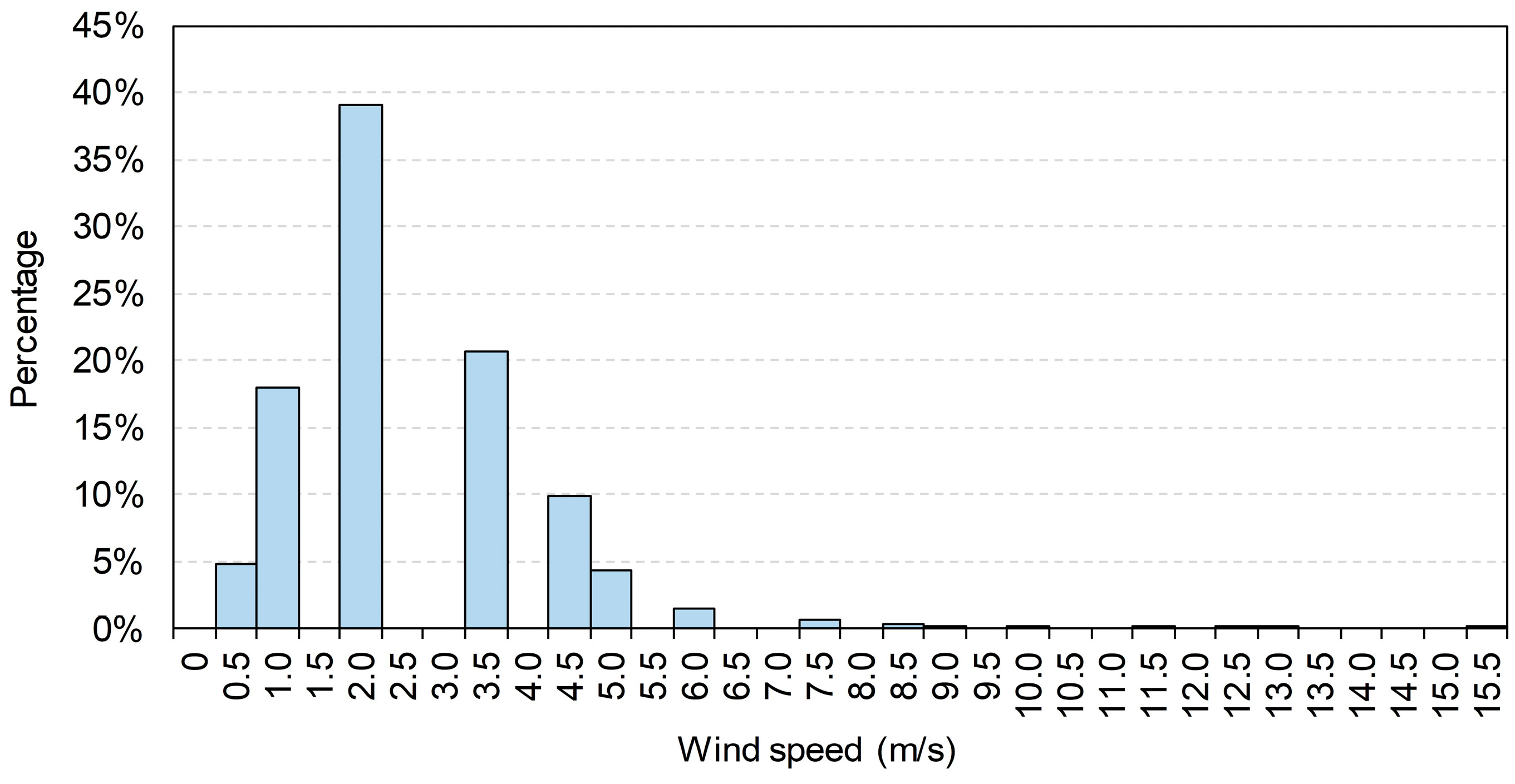
The weather data website (https://gis.ncdc.noaa.gov/maps/ncei/cdo/hourly) administrated by the National Oceanic and Atmospheric Administration (NOAA) provides users with free global wind data recorded at hourly intervals. In this study, the hourly wind speed data for Wuhan from 1 January 2019, to 31 March 2019, was used as the representative wind condition for Wuhan during the service period of the Huoshenshan Hospital. The distribution of wind speed data is shown in Figure 14. The median value is 1.90 m/s, and the proportion of wind speed not exceeding 5 m/s reaches 97%. Therefore, in the subsequent analysis of cases with different wind speeds, the wind speed at the height of 10 m was taken as 0.5, 1.9, 3.5, and 5.0 m/s, respectively, to cover the wind speed range to the maximum extent. For ease of expression, the cases with different wind speeds and directions are correspondingly named as Case-S-D hereinafter, where S represents the wind speed (i.e., 0.5, 1.9, 3.5, and 5.0 m/s) while D represents the wind direction (i.e., N, NE, E, SE, S, SW, W, and NW). According to

Table A2. Classification of the aerodynamic roughness length, z₀ [33].

z0 (m)	Classification	Landscape
0.0002	sea	sea, paved areas, snow-covered flat plain, tidal flats, smooth desert
0.005	smooth	beaches, pack ice, snow-covered fields
0.03	open	grass prairie, farm fields, tundra, airports, heather
0.1	roughly open	low crops and occasional obstacles (single bushes)
0.25	rough	high crops, scattered obstacles such as trees or hedgerows, vineyards
0.5	very rough	mixed farm fields and forest clumps, orchards, scattered buildings
1.0	closed	suburbs, villages, forests
>2	chaotic	large towns and cities, irregular forests

and

Table A3. Suggested values of the Obukhov length, L [33].

Thermal Stability of the Atmosphere	Value Range (m)	Suggested Value (m)
very unstable	−200 ≤ L < 0	−100
unstable	−500 ≤ L < −200	−350
neutral	|L| > 500	1,000,000
stable	200 < L ≤ 500	350
very stable	0 < L ≤ 200	100

in Appendix B, the aerodynamic roughness length, z₀, and the Obukhov length, L, were taken as 0.1 m and 350 m, respectively, to define the mean wind speed profile in the FDS.

4.2. Conceptual Design

In the conceptual design phase, designers of the Huoshenshan Hospital were to adopt a building configuration similar to that of Beijing Xiaotangshan temporary hospital (located in Changping District, Beijing), which has been proven effective during the SARS outbreak in 2003. The FDS model (see Figure 15) of the conceptual design was rapidly constructed by utilizing the FDSGenerator program.

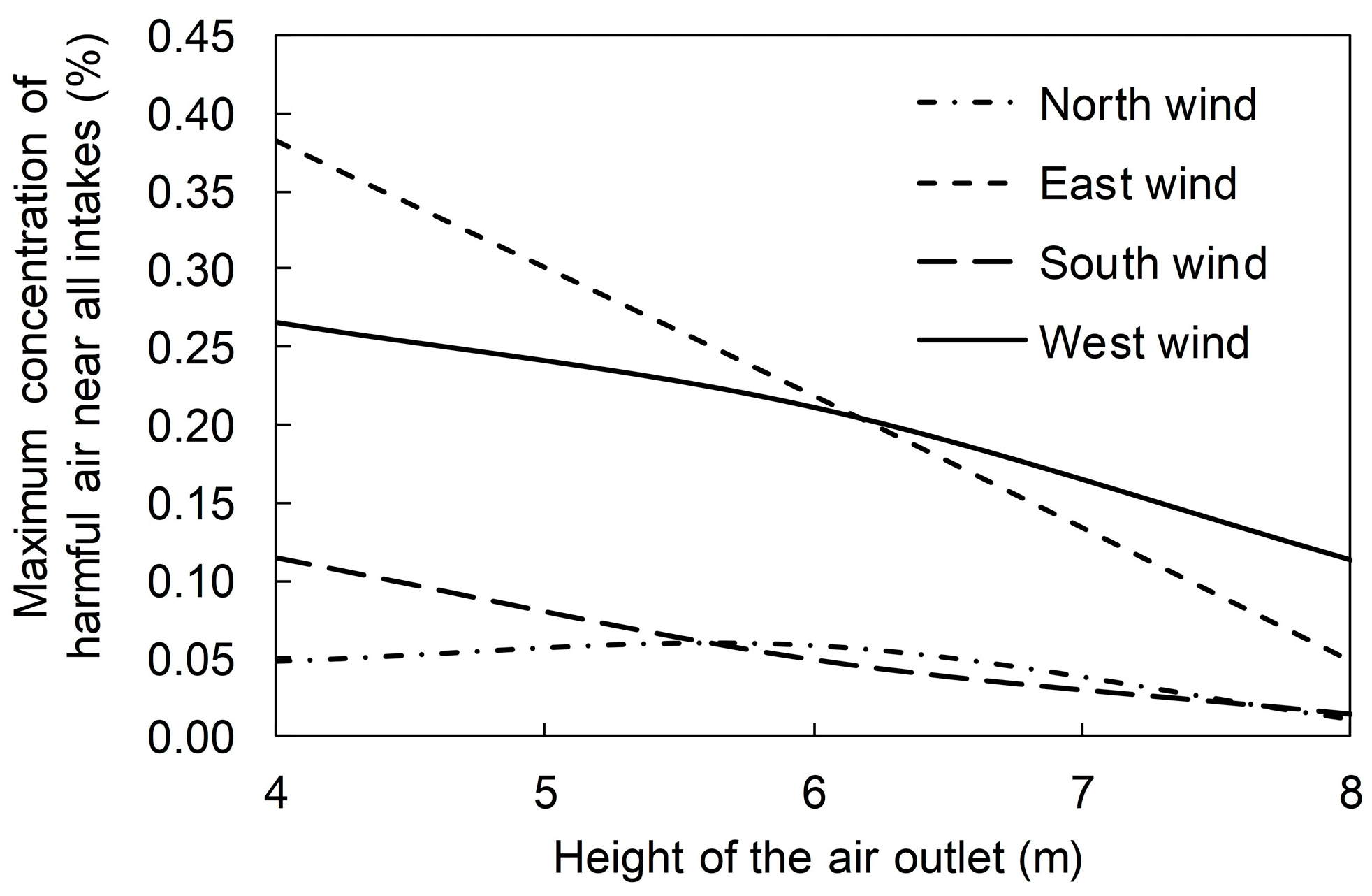
Considering that the height of the air outlet may have significant effects on other aspects of the final design scheme, the proposed simulation method was adopted to determine a suitable height range for the air outlet. Figure 15 shows the locations of air outlets and fresh-air intakes in the conceptual design. The height of the fresh-air intake was taken as 2 m, while several air outlet heights ranging from 4 m to 8 m were considered. To reduce analysis time, only cases with wind speeds of 1.9 m/s (i.e., Case-1.9-N, Case-1.9-E, Case-1.9-S, and Case-1.9-W) were modeled and simulated in this design phase. The volume of each air outlet was taken as 0.5 m³/s.

The computational domain covered a volume of 300 m × 300 m × 30 m, which is in agreement with the AIJ [38] best practice guideline. In terms of the grid scheme, the grid size of the domain under the height of 12 m was set to 0.5 m × 0.5 m × 0.5 m, whereas that of the remaining domain was set to 1.0 m × 1.0 m × 1.0 m. The total number of cells was 1.026 × 10⁷. According to the FDS user guide [33], the “PERIODIC” boundary condition was adopted for the inlet, outlet, and lateral boundaries, while the “GROUND” and “OPEN” boundary conditions were used for the ground and top boundary, respectively. The total simulation time was set as 400 s, of which the first half was used to achieve a stable flow field while the remaining half was used to record the concentration data of the exhausted harmful air at the monitoring points near fresh-air intakes.

Given that the knowledge of the transmission mechanism of SARS-CoV-2 was quite limited during the design of the Huoshenshan Hospital, it was challenging for engineers to quantify the effect of filtration devices on pollutant concentration. As a result, the function of filtration devices was ignored in all simulations introduced in Section 4, which would facilitate a safer design of the hospital. Provided that the harmful air concentration at the air outlet was defined as 100%, the relationship between the maximum value of the time-averaged concentrations near all fresh-air intakes and the air outlet height can be illustrated by Figure 16. It can be seen that the maximum harmful air concentration near all the fresh-air intakes decreases with the increase in the height of the air outlet. When the air outlet height reaches 8 m, the maximum harmful air concentration near all intakes can be reduced to approximately 0.1% of that at the air outlets.

4.3. Evaluating the Design Scheme of the Air Outlets and Fresh-Air Intakes

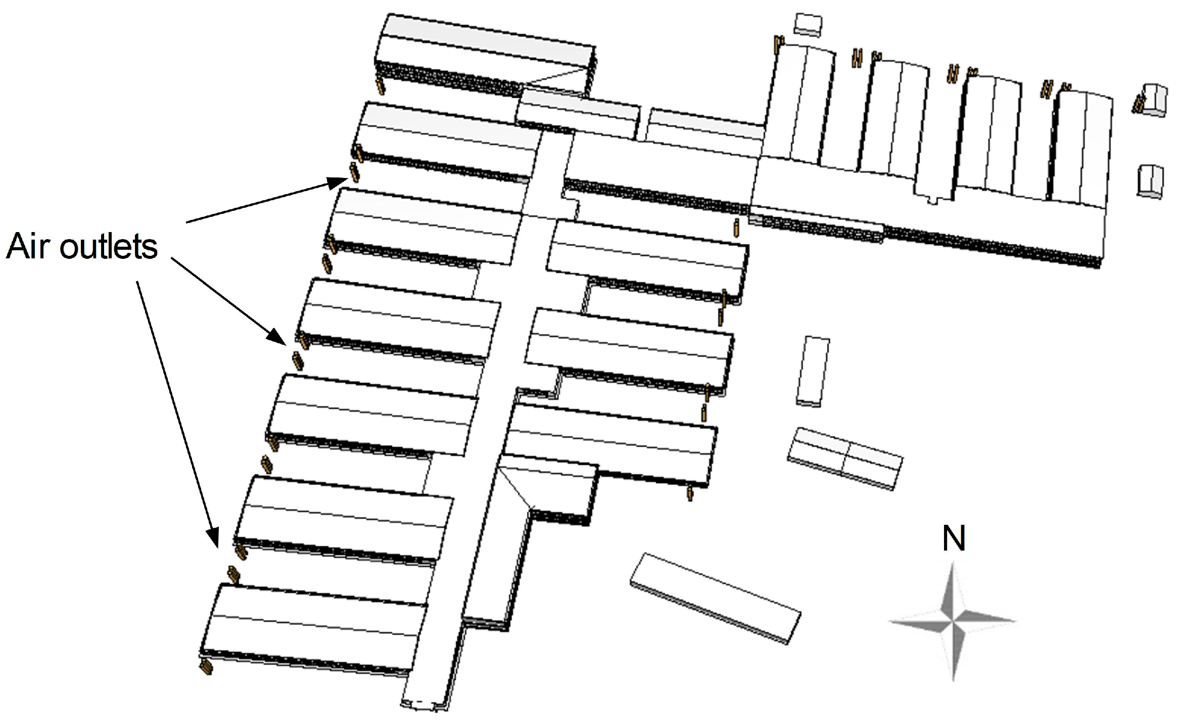
According to the simulation results of the conceptual designs, the air outlet heights for the hospital were designed as 8 m and 10 m. The fresh-air intakes were mainly distributed at the height of 2 m, while a few of the intakes were arranged at the heights of 3.9 m and 7.0 m due to construction constraints. The air outlets were located at the end of the ward building, while the fresh-air intakes were mainly distributed in the middle of the ward building. Based on the SketchUp model constructed by the design agency, the FDS model shown in Figure 17 was constructed through the modeling method introduced in Section 2.1.3. The numbers of air outlets and monitoring points near fresh-air intakes were 52 and 141, respectively. In the FDS model, the pollutant release rate for each air outlet was determined based on the HVAC design results of the Wuhan Huoshenshan Hospital, and then the mass fraction of harmful air for each air outlet was calculated through Equation (1).

As the hospital is approximately 360 m × 320 m in size with a height of 12 m for the tallest building, a computational domain of 680 m × 640 m × 80 m was constructed, which is in agreement with the AIJ [38] best practice guideline. In terms of the grid scheme, the grid size of the domain under the height of 25 m was set to 0.5 m × 0.5 m × 0.5 m. The grid size of the domain between the heights of 25 m and 50 m was set to 1.0 m × 1.0 m × 1.0 m, while that of the remaining domain was set to 2.0 m × 2.0 m × 2.0 m. The total number of cells is 9.955 × 10⁷. According to the FDS user guide [33], the “PERIODIC” boundary condition was adopted for the inlet, outlet, and lateral boundaries, while the “GROUND” and “OPEN” boundary conditions were used for the ground and top boundary, respectively.

4.3.1. Cases with Different Wind Directions

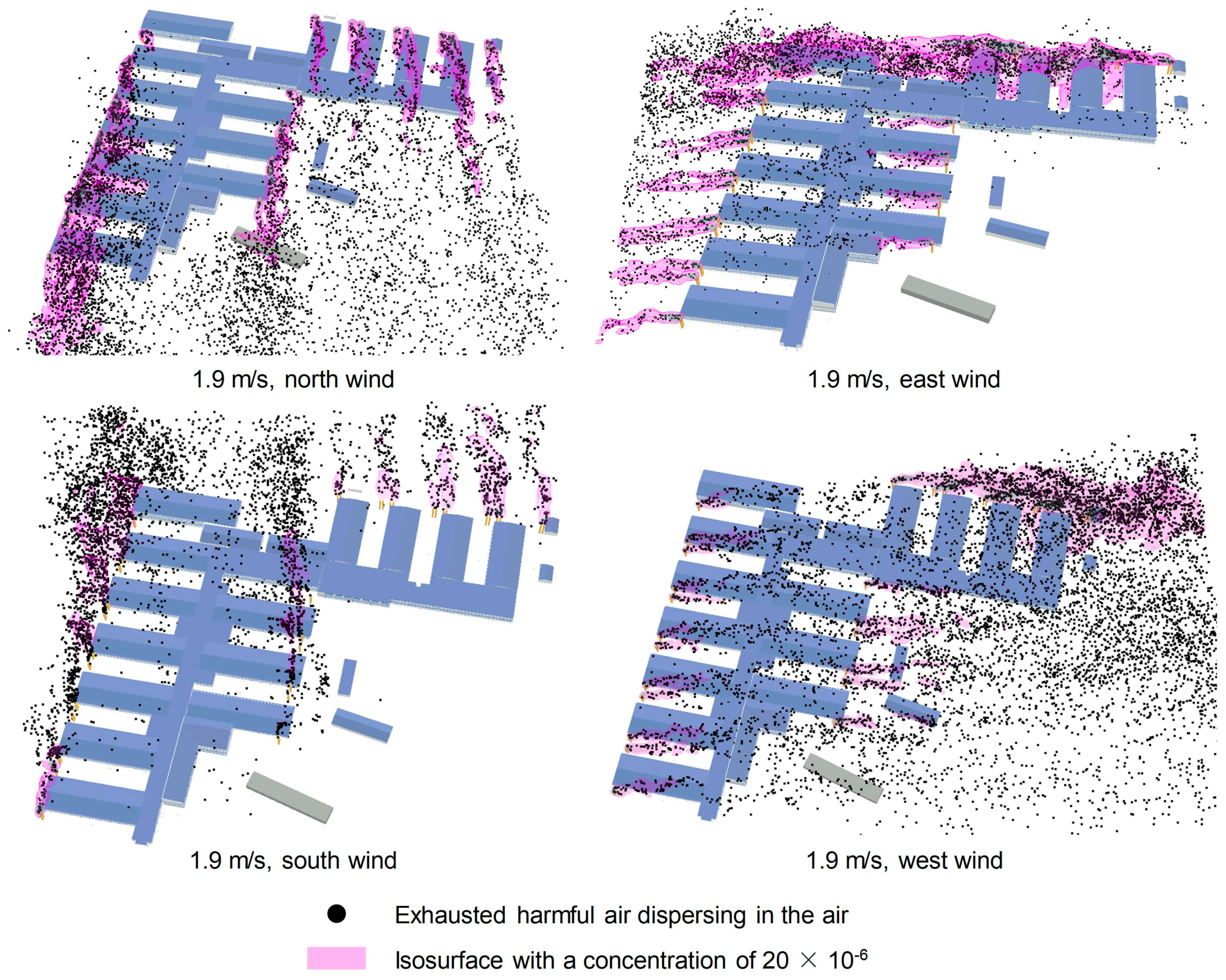
Provided that the wind speed at the height of 10 m was 1.9 m/s, cases with eight wind directions (i.e., Case-1.9-N, Case-1.9-NE, Case-1.9-E, Case-1.9-SE, Case-1.9-S, Case-1.9-SW, Case-1.9-W, and Case-1.9-NW) were simulated to investigate the most unfavorable wind direction. Figure 18 shows the typical visualizations of the harmful air dispersion under four wind directions, where the black particles represent the exhausted harmful air dispersing in the air, and the pink curved surfaces represent the isosurfaces with a concentration of 20 × 10⁻⁶. This type of high-fidelity visualization can assist designers to more intuitively investigate the distribution characteristics of harmful air around the temporary hospital, thereby helping designers to compare and optimize design schemes in an improved manner.

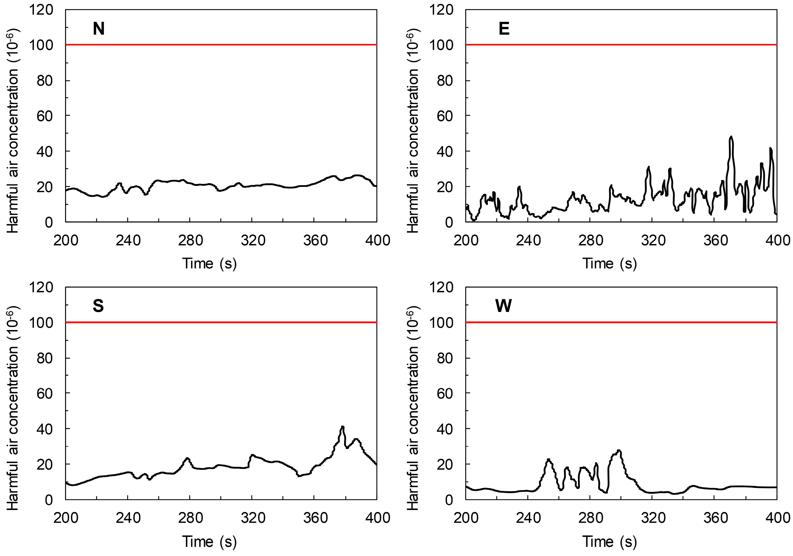
In this study, the infectivity data relating to SARS was adopted as a reference for the infectivity of SARS-COV-2, given that scientists over the world did not have a unified understanding of the infectivity of the virus during the design period of the hospital. According to Jiang et al. [1], if the air emitted from a SARS patient is diluted to more than 10,000 times using clean air, it would result in a low risk of infection. Hence, in this study, it was assumed that if the concentration of the exhausted harmful air is less than 100 × 10⁻⁶, the harmful air would be accompanied by a low risk of infection. Figure 19 shows the typical time–history data of the harmful air concentration near the specific fresh-air intake with the highest instantaneous concentration under four wind directions. In the conditions with wind speeds of 1.9 m/s, the maximum concentrations of harmful air near fresh-air intakes under eight wind directions are all lower than 100 × 10⁻⁶, indicating that the exhausted harmful air from air outlets results in a low risk of infection to the fresh-air intakes.

4.3.2. Cases with Different Wind Speeds

According to the simulation results of cases with different wind directions, east and northwest wind directions were considered as the most unfavorable wind directions. Therefore, under the conditions of these two wind directions, the simulation of cases with different wind speeds (i.e., Case-0.5-E, Case-3.5-E, Case-5.0-E, Case-0.5-NW, Case-3.5-NW, and Case-5.0-NW) were performed to investigate the effect of the wind speed on the harmful air concentrations near the fresh-air intakes.

The maximum instantaneous concentrations of harmful air near fresh-air intakes under different wind speeds are all lower than 70 × 10⁻⁶ (see

Table 1. Maximum instantaneous concentrations of harmful air near fresh-air intakes under different wind speeds.

Wind Speed		0.5 m/s	1.9 m/s	3.5 m/s	5.0 m/s
Maximum Instantaneous Concentration	East wind	47.004 × 10−6	48.289 × 10−6	55.754 × 10−6	42.501 × 10−6
	Northwest wind	33.096 × 10−6	62.311 × 10−6	40.017 × 10−6	30.084 × 10−6

). According to the simulation results of all cases, the maximum instantaneous concentration of 62.311 × 10⁻⁶ occurs in Case-1.9-NW. It should be noted that the function of filtration devices was neglected in these simulations. As a result, the actual concentrations of harmful air near the fresh-air intakes should be lower than the simulation results. In conclusion, the design scheme of the Wuhan Huoshenshan Hospital can ensure that the exhausted harmful air from air outlets does not have an adverse impact on the fresh air at intakes.

4.4. Evaluating the Impact of Exhausted Harmful Air from the Temporary Hospital on the Surrounding Environment

The Wuhan Huoshenshan Hospital is located in an area where there are also several residential buildings. Hence, except for ensuring that the exhausted harmful air from air outlets does not cause an adverse impact on the fresh-air intakes, it is also necessary to quantify the impact of the harmful air on the surrounding environment. As shown in Figure 20, there is a cluster of villas and several high-rise residential buildings to the north and northwest of the hospital, respectively. Additionally, there are some hotels located in the southern section of the target area. Since hotels were closed for the sake of safety when the hospital was in operation, this study focused on the impacts of the exhausted harmful air, from the hospital, on the surrounding high-rise building and villas.

The FDS model of the target area was constructed through the high-efficiency modeling method introduced in Section 2.1.4. In the complete FDS model, the hospital was modeled based on the pre-constructed SketchUp model, while the surrounding buildings were modeled using the GIS data captured from public mapping sources. In the FDS model, the pollutant release rate for each air outlet was determined based on the HVAC design results of the Wuhan Huoshenshan Hospital. Then the mass fraction of harmful air for each air outlet was calculated through Equation (1). The plane positions of the monitoring points for the purpose of recording the harmful air concentration data near the high-rise buildings and villas are shown in Figure 20. Given that the average height of the villas and high-rise buildings is approximately 7 m and 30 m, respectively, the monitoring points around the villas are located at heights of 1.5 m and 5 m while those around the high-rise buildings are located at several heights ranging from 1.5 m to 26.0 m (i.e., 1.5, 5.0, 8.5, 12.0, 15.5, 19.0, 22.5, and 26.0 m). Totally 432 monitoring points were identified for this model.

As the target area is approximately 730 m × 740 m in size with a height of 36 m for the tallest building, a computational domain of 1680 m × 1680 m × 235 m was constructed, which is in agreement with the AIJ [38] best practice guideline. The whole computational domain was divided into five parts: (1) the subdomain under the height of 55 m, (2) the subdomain between the heights of 55 m and 75 m, (3) the subdomain between the heights of 75 m and 115 m, (4) the subdomain between the heights of 115 m and 155 m, and (5) the subdomain above the height of 155 m. The grid size of the five subdomains is 1 m × 1m × 1 m, 2 m × 2 m × 2 m, 4 m × 4 m × 4 m, 8 m × 8 m × 8 m, and 16 m × 16 m × 16 m, respectively. The total number of cells was 1.643 × 10⁸. According to the FDS user guide [33], the “PERIODIC” boundary condition was adopted for the inlet, outlet, and lateral boundaries, while the “GROUND” and “OPEN” boundary conditions were used for the ground and top boundary, respectively.

4.4.1. Cases with Different Wind Directions

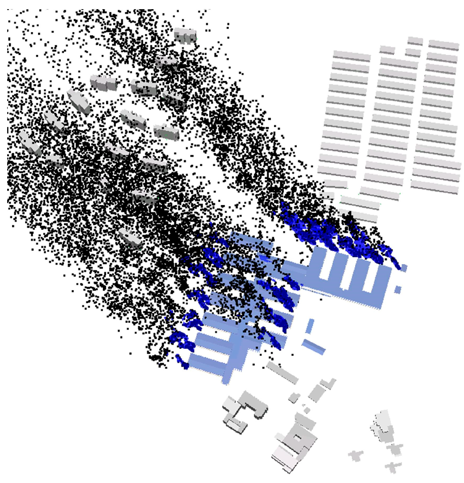
Provided that the wind speed at the height of 10 m was 1.9 m/s, cases with eight wind directions (i.e., Case-1.9-N, Case-1.9-NE, Case-1.9-E, Case-1.9-SE, Case-1.9-S, Case-1.9-SW, Case-1.9-W, and Case-1.9-NW) were simulated. The simulation results indicated that under four wind directions (i.e., east wind, southeast wind, south wind, and southwest wind), the surrounding high-rise buildings and villas would be affected by the exhausted harmful air from the hospital. Figure 21 shows the typical visualization of the harmful air dispersion under the southeast wind, where the black particles represent the exhausted harmful air dispersing in the air, and the purple curved surfaces represent the isosurfaces with a concentration of 20 × 10⁻⁶. In the cases with wind speeds of 1.9 m/s, the maximum concentration of harmful air near surrounding buildings under different wind directions are all lower than 40 × 10⁻⁶, provided that the function of filtration devices is neglected.

4.4.2. Cases with Different Wind Speeds

Under the abovementioned four wind directions, the cases with different wind speeds (i.e., Case-0.5-D, Case-3.5-D, and Case-5.0-D, where D represents E, SE, S, and SW, respectively) were further modeled and simulated. As shown in

Table 2. Maximum instantaneous concentrations of harmful air around surrounding buildings under different wind speeds.

Wind Speed		0.5 m/s	1.9 m/s	3.5 m/s	5.0 m/s
Maximum instantaneous concentration	East wind	10.699 × 10−6	20.560 × 10−6	11.879 × 10−6	9.019 × 10−6
	Southeast wind	16.576 × 10−6	14.819 × 10−6	7.187 × 10−6	7.811 × 10−6
	South wind	32.637 × 10−6	37.370 × 10−6	29.561 × 10−6	22.874 × 10−6
	Southwest wind	20.604 × 10−6	21.025 × 10−6	18.531 × 10−6	10.586 × 10−6

, the maximum instantaneous concentration of harmful air near surrounding buildings under different wind speeds are all much lower than 100 × 10⁻⁶. In all cases, the maximum instantaneous concentration of 37.370 × 10⁻⁶ occurs in Case-1.9-S. It should be noted that the function of filtration devices was neglected in these simulations. Therefore, the actual concentrations of harmful air near surrounding buildings should be lower than the simulation results. In conclusion, the design scheme of the Wuhan Huoshenshan Hospital can ensure that the exhausted harmful air does not have an adverse impact on the surrounding environment.

4.5. Differences between the Simulation Results in the Transition and Final Design Phases

It should be noted that the surrounding buildings considered in the final design phase may have an impact on the simulation results of the maximum instantaneous concentrations near the fresh-air intakes. Hence, the simulation cases with wind speeds of 1.9 m/s in the transition and final design phases, which have been introduced in Section 4.3.1 and Section 4.4.1, are used here to compare the maximum instantaneous concentrations of exhausted harmful air near the fresh-air intakes between the final design phase (surrounding buildings are considered) versus the transition design phase (the neighborhood is not included).

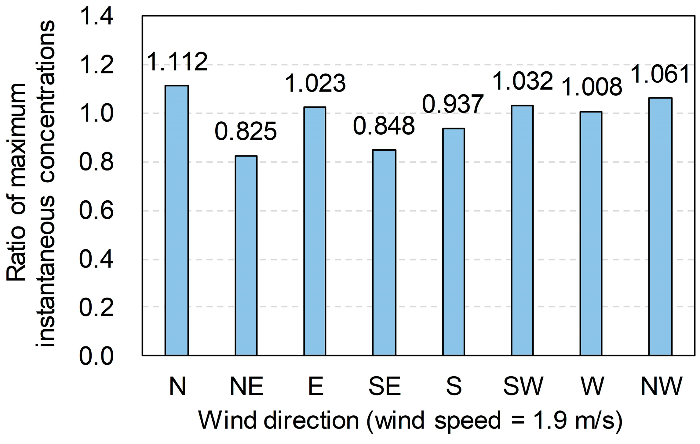
Figure 22 shows the differences between the simulation results of the two design phases. In the figure, the height of the column indicates the ratio of the simulated maximum instantaneous concentration near the fresh-air intakes in the final design phase to that in the transition design phase. It can be seen that for the east, southwest, and west wind directions, the relative changes of the simulated maximum instantaneous concentrations are within 5%. Hence, it is considered that for these three wind directions, the surrounding buildings considered in the final design phase do not have an obvious impact on the simulation results of the maximum instantaneous concentrations near the fresh-air intakes, given the random nature of the calculation in CFD. The relative changes of the simulated maximum instantaneous concentrations for the south and northwest wind directions are in the range of 5% to 10%, while those for the north, northeast, and southeast wind directions are in the range of 10% to 20%. It means that for these five wind directions, the impact of the surrounding buildings on the simulation results should not be neglected during the transition design phase. For all wind directions, the maximum relative change of the simulated maximum instantaneous concentration is 17.5%. And in the final design phase, the maximum instantaneous concentration of 66.112 × 10⁻⁶ occurs in Case-1.9-NW, which is consistent with the conclusion drawn from the simulations in the transition design phase. Furthermore, it needs to be noted that although the simulations in the transition design phase did not consider the influence of surrounding buildings, it is still very necessary to perform such simulations to help engineers look into the pros and cons of different design schemes as quickly as possible.

5. Conclusions

The spread of COVID-19 has caused severe impacts in China and many other countries around the world. Different design schemes of the COVID-19 temporary hospitals need to be quantitatively evaluated and optimized in a short time span, which calls for a high-efficiency and low-cost methods to simulate the dispersion of the exhausted harmful air from temporary hospitals. To address this problem, a high-efficiency simulation framework based on the FDS was proposed in this study. The proposed simulation framework adapts to building information with different LODs in various design phases of the temporary hospital and has been applied in the design of the Wuhan Huoshenshan Hospital, the first temporary hospital built in China for centralized treatment of the COVID-19 patients. The main conclusions of this study are as follows:

(1)

Powered by the FDSGenerator program, the open-source feature of FDS, and the cloud computing technology, the proposed simulation method can assist engineers in quickly investigating the spatial distribution of the exhausted harmful air from temporary hospitals, thereby enabling designers to complete the HVAC design in a short time. The high-efficiency simulation framework and the corresponding case study of the Wuhan Huoshenshan Hospital can provide a reference for the HVAC design and overall planning of similar hospitals in China and other affected countries.

(2)

In terms of the numerical simulation of pollutant dispersion around buildings, compared with the commercial CFD software Fluent, FDS can significantly improve the modeling and CFD computation efficiency while ensuring accuracy.

(3)

According to the simulation results of the Wuhan Huoshenshan Hospital, neither the fresh-air intakes nor the surrounding buildings would be polluted by the harmful air discharged from the air outlets of the hospital.

At present, COVID-19 is still rapidly spreading in many countries around the world. The proposed high-efficiency simulation framework and the corresponding case study of the Wuhan Huoshenshan Hospital can provide a reference for the design and overall planning of similar hospitals in some affected countries. Furthermore, even not in the COVID-19 era, the proposed simulation method can also be a useful design tool for some infectious disease hospitals.