Abstract
Instance selection and construction methods were originally designed to improve the performance of the k-nearest neighbors classifier by increasing its speed and improving the classification accuracy. These goals were achieved by eliminating redundant and noisy samples, thus reducing the size of the training set. In this paper, the performance of instance selection methods is investigated in terms of classification accuracy and reduction of training set size. The classification accuracy of the following classifiers is evaluated: decision trees, random forest, Naive Bayes, linear model, support vector machine and k-nearest neighbors. The obtained results indicate that for the most of the classifiers compressing the training set affects prediction performance and only a small group of instance selection methods can be recommended as a general purpose preprocessing step. These are learning vector quantization based algorithms, along with the Drop2 and Drop3. Other methods are less efficient or provide low compression ratio.
1. Introduction
Classification is one of the basic machine learning problems, with many practical applications in industry and other fields. The typical process of constructing a classifier consists of data collection, data preprocessing, training and optimizing the prediction models and finally applying the best of the evaluated models. The described scheme is obvious, however we face two types of problems. The first one is that recently we more often start to construct classifiers with limited resources and the second one is that we want to interpret and understand the data and the constructed model easily.
The first group of restrictions are mostly related to time and memory constraints, where machine learning algorithms are often trained on mobile devices or micro computers like Rasberry Pi and other similar devices. There are basically three approaches to overcome these restrictions:
- using specially tailored algorithms which are designed to face those challenge
- limiting the size of the training data
- exporting the training process from the device to the cloud or other high performance environment
In the paper we focus on the second approach where instead of redesigning the classification algorithm or sending the data to the cloud we analyze how the data filters or in other words how the training set reduction methods influence classification performance with the data processing pipeline depicted in Figure 1.
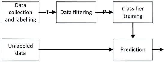
Figure 1.
The pipeline of prediction model construction with data filtering.
The data filter has two goals: first it can improve the classifier performance by eliminating noisy samples from the training data thus allowing to achieve higher classification accuracy, and the second goal is training set compression. Training set size reduction allows to speed up classifier construction process but also it speeds up decision making when the classifier is already trained [1]. The speed up in classifier training is rather obvious when the size of the input data is smaller but the speed up in the prediction phase results from smaller number of support vectors of the support vector machine, shallow trees (earlier stopping of tree construction) and lower number of reference vectors in kNN. Moreover, it speeds up model selection and optimization. Here, the gain should be multiplied by the number of evaluated classifiers and their hyper-parameters, because the filtering stage is applied once and then the classifier selection and optimization is carried out.
Training set compression can be also used for solving model interpretability where the so called prototype-based rules [2,3] can be applied. These rules are also based on limiting the size of the data. And in this case, even if the original dataset is small, further limiting dataset size is still beneficial.
The main purpose of the paper and the research objective is the analysis of both aspects of data filtering that is the influence on prediction accuracy of various classifiers and the influence on training set size reduction.
In the study we evaluate a set of 20 most popular instance selection and construction methods used as data filters and 7 popular classifiers on 40 datasets in terms of classification performance and training set compression. The evaluated data filters are: condensed nearest neighbor (CNN), edited nearest neighbor (ENN), repeated-edited nearest neighbor (RENN), All-kNN, instance based learning version 2 (IB2), relative neighbor graph editing (RNGE), Drop family, iterative case filtering (ICF), modified selective subset selection (MSS), hit-miss network editing (HMN-E), hit-miss network interactive editing (HMN-EI), class conditional instance selection (CCIS) as well as learning vector quantization version 1,2.1 (respectively LVQ1, LVQ2.1), generalized learning vector quantization (GLVQ), k-Means. These data filters are selected for the evaluation, because they are the most frequently used instance selection methods. The datasets after filtering are used to train classifiers such as k-nearest neighbor (kNN), support vector machine (SVM), decision tree based methods, linear model and simple Naive Bayes. The hyperparameters of each of these classifiers are optimized with the grid search approach in order to achieve the highest possible prediction accuracy on the compressed data. Moreover, the obtained results are compared to the results obtained with simple stratified random sampling, which defines an acceptance threshold below which particular methods are not beneficial for given classifiers.
The article is structured as follow: in the next section an overview of instance selection methods is provided, with a literature overview, and also the research gap is presented, then in Section 3 we describe the experimental setup, and in Section 4 the results are presented. Finally, Section 5 summarizes the paper with general conclusions.
2. Research Background
2.1. Problem Statement
From the statistical point of view, reduction of the training set size will not affect prediction accuracy of the final classifier when the conditional probability of predicting class c for given vector remains unchanged when estimated from the original training set and from the set of prototypes obtained from the data filtering process.
In the literature one of popular multidimensional probability estimation methods is based on the nearest neighbor approach [4]. Similarly, for kNN many data filtering methods were developed in order to select a suitable subset of the training set. These methods are called instance selection methods and instance construction or prototype generation methods, and mostly they were designed to overcome weaknesses of the kNN classifier. In instance selection, usually the performance of kNN or even 1-NN classifier is used to identify those training samples which are important for the classification. These are mostly border samples close to the decision boundary. Instances which represent larger groups of instances from the same class and noise samples are usually filtered out because they reduce the performance of kNN. On the other hand, instance construction methods tend to find optimal position of the stored samples by 1-NN, so they do not need to represent samples from the original training set, these are usually new samples. An example effect of applying instance selection methods to the training set is presented on Figure 2.
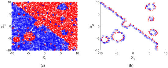
Figure 2.
Example effect of artificial 2D training set compression using Drop3 instance selection methods. (a) Original training set with additional noise (b) Training set after compression.
The idea of applying instance selection and prototype generation methods as data filters is not new and it is often considered a standard preprocessing step. In particular in Reference [5] some of the instance selection methods evaluated in our study were considered as the most effective preprocessing methods.
For example we have applied instance selection in the optimization of metallurgical processes for data size limitation and rule extraction [6,7], but instance selection methods were also applied in haptic modeling [8] as well as for automatic machine learning [9]. However, we cannot find in the literature any comprehensive study analyzing the influence of the instance selection methods on various classifiers. Most of the authors when presenting new algorithms indicate only the performance of 1-NN, kNN with fixed k parameter, and sometimes other classifiers but usually also with fixed hyperparameters. Such a comparison can be considered unfair, because the training set is being changed during the data filtering so different parameters are required by the classifiers. Unfortunately, such a comparison requires much larger computational time especially when using grid search with internal cross-validation procedure, so the process is usually simplified and only classifiers with fixed parameters are used. Only in References [10,11] some broader comparison is available but the experiments were conducted on only few (6 and 8) datasets. To fill that gap we provide a detailed analysis of the influence of the data based on instance selection and construction methods applied to 40 datasets.
2.2. Instance Selection and Construction Methods Overview
One of the most important properties of data filtering methods is the relation between instances in the original training set and the in the selected prototype set . If then the methods are called instance selection algorithms, because the prototypes are selected directly from the training set . This property does not hold for prototype construction also called prototype generation methods. In this case the elements of are new vectors which can constitute completely new instances, which have never appeared in .
This property is important considering the comprehensibility of the selected samples. In the case of instance selection methods the instances can be mapped into real objects, while in the case of instance construction methods the direct mapping is not possible. This is especially important when working with prototype-based rules [2,12], or other interpretable models.
In the literature perhaps the best overview of instance selection methods can be found in Reference [13] where the authors provide a taxonomy of over 70 instance selection methods, and empirically compare half of them in terms of compression and prediction performance of 1-NN classifier. The same group of authors of Reference [14] perform a similar analysis for prototype generation methods where 32 methods are discussed and 18 of them are empirically compared in application only for 1-NN classifier.
The taxonomy of data filtering methods can be presented in the following aspects:
- search direction
- −
- incremental, when given method starts from an empty set and iteratively adds new samples, such as in CNN [15] or IB2 [16]
- −
- decremental, when a given method starts from and then samples from are iteratively removed such as in HMN-E and HMN-EI [17], MSS [18], Drop1, Drop2, Drop3 and Drop5 [19], RENN [20].
- −
- batch, when the instances are removed at once after analysis of the input training set. An examples of such methods are ENN [21], All-kNN [20] RNGE [22], ICF [23], CCIS [24].
- −
- fixed, when a fixed number of prototypes is given as the hyperprarametr of the method. This group includes LVQ (LVQ1, LVQ2.1, GLVQ) family [25,26], k-Means and random sampling.
- type of selection
- −
- condensation, when the algorithm tries to remove samples, which are located far from the decision boundary, as in the case of IB2, CNN, Drop1 and Drop2, MSS.
- −
- edition, when the algorithm is designed for noise removal, such as ENN, RENN, All-kNN, HMN-E.
- −
- hybrid, when the algorithm performs both steps—condensation and edition. Usually these methods starts from noise removal, and then perform condensation. This group includes: Drop3, Drop5, ICF, HMN-EI.
- the evaluation method
- −
- filters, where the method uses internal heuristic independent to the final classifier.
- −
- wrappers, when external dedicated classifier is used to identify important samples.
The decision of assigning an algorithm to the right evaluation method depends on the final prediction model applied after data filtering. If the instance selection or construction method is followed by 1-NN or kNN classifier they can be considered as wrappers, because internally all of them use a kind of nearest neighbor based approach to decide whether an instance should be selected or rejected. On the other hand they can be also considered as filters, when the data filter takes as input entire training set and returns selected subset which is then used to train any classifier, not only the kNN. There are implementations which works as wrappers, so they allow to use all kind of classifiers such as in Reference [27], where instead of kNN any other classifier can be used, in particular the MLP neural network was used. The drawback of the wrappers is the increase of computational complexity. Here in this article we only consider the standard instance selection methods without any generalization.
3. Experimental Design
There are several factors which determine the applicability of given algorithms as a general purpose training set filter. Among the most important are compression level and prediction accuracy of the final classifier. The compression is defined as:
so that higher value of compression indicates that more samples were rejected and the resultant set is smaller and lower values (close to 0) indicates that the output training set is larger. The second property is the prediction accuracy of the classifier trained on . This value is subjective to the applied classifier, so that for one classifier given set may result in high accuracy, while for the other the accuracy can be worse. Here a simple accuracy measure was evaluated:
In order to determine the applicability of instance selection and construction methods as universal training set filters we designed experiments which mimic typical use cases of training set filtering. The scheme of the data processing pipeline is presented in Figure 3
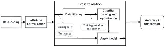
Figure 3.
The pipeline of data processing used in the experiments.
It starts with data loading and attribute normalization, then the 10 fold cross-validation procedure is executed which wraps the data filtering stage (our instance selection or construction method) followed by classifier training and hyperparameter optimization procedure. Finally, the trained classifier is applied to the test set. During the process execution prediction accuracy and compression were recorded.
In the experiments the most commonly used classifiers were evaluated. These are: the basic classifiers for which the evaluated data filters were designed such as 1-NN and kNN; simple classifiers like Naive Bayes or linear model (GLM); followed by kernel methods such as SVM with Gaussian kernel and finally the decision tree based methods including C4.5 and Random Forest. Many of these methods require careful parameter selection such as the value of k in kNN or C and in SVM or the number of trees in Random Forest. All of the evaluated parameters are presented in Table 1. It is important to note that each of the applied data filters was independently evaluated for each classifier, because a particular filter may be beneficial for one classifier and unfavorable for another.

Table 1.
Parameter settings of the evaluated classifiers.
The entire group of instance selection and construction methods is very broad. As indicated in Section 2.2 some authors distinguish over 70 instance selection methods and over 32 prototype construction methods [13,14]. From these groups we selected the most popular ones which can be found in many research papers as the reference methods [10,11,28,29,30]. These are CNN, ENN, RENN, All-kNN, IB2, RNGE, Drop1, Drop2, Drop3, Drop5, ICF, MSS, HMN-E, HMN-EI, CCIS, from the group of instance selection methods, and from the group of prototype generation methods we selected 3 algorithm from the family of LVQ algorithms, these are LVQ1, LVQ2.1, as well as the GLVQ algorithm. In the experiments we also evaluated k-Means clustering algorithm which is most often used to reduce the size of the training set [31]. The k-Means algorithm was independently applied to each class label, and then the obtained cluster centers were used as prototypes with appropriate class labels [32]. All of the prototype generation methods belong to the group of fixed methods, so they require to determine the compression manually. For that purpose the experiments were carried out for two different initial sets of prototypes: randomly selected of the training samples used for initialization which corresponds to compression and also of the training samples which corresponds to compression. The compression is the lower bound of the compression obtained by most of instance selection methods.
All evaluated methods were also compared with the random stratified sampling (Rnd), which is the simplest solution that can be used as a data filter. Similarly as with prototype construction methods, the experiments with Rnd were conducted for compression and that corresponds to Rnd(0.3) and Rnd(0.1) (the numbers represent percentage of the samples that remain). The accuracy obtained for Rnd constitute the lower bound which allows to distinguish beneficial data filters from the weak ones that are worse than simple random sampling.
The experiments were carried out on 40 datasets obtained from the Keel repository [33]. A list of the datasets is presented in Table 2. All the calculations were conducted using RapidMiner software with Information Selection extension developed by the authors [34]. The extension is available at the RapidMiner Marketplace and the most recent version is also available at GitHub (https://github.com/mblachnik/infoSel). Some of the evaluated algorithms like HMN-EI and CCIS were taken from the Keel framework [35] and integrated with the Information Selection extension.
Table 2.
Datasets used in the experiments. The s/a/c denotes the number of samples, attributes and classes.
4. Results and Analysis
Since simple averaging has limited interpretability, we used both average performance and average rank to asses the quality of the evaluated methods. In order to make ranking for each dataset and each classifier the results obtained for particular data filters were ranked from the best to the worst in terms of classification accuracy and compression. The highest rank (equal to 26, which is the number of evaluated algorithms) was given to the best filter method for particular dataset and the lowest rank (1) was assigned to the worst method (rank with ties). Then the ranks over datasets were averaged to indicate the final performance. Such a comparison does not reflect how much one method differs from the other in terms of given quality measure, but ranking unlike averaging performances is insensitive to the data distribution where measures like accuracy can range from 40% on one dataset up to 99% on another. On the other hand ranking do not provide information on how much the methods differ so these both quality measures complement each other and should be considered together, where the ranking gives an answer which method was more often better, and then, the mean performance indicates how much given method was better from the competitor. Moreover, the threshold obtained by the random sampling should be applied simultaneously to both values and when any of them is below the threshold given method should be rejected as useless.
The obtained results including both average ranks as well as average performances are presented in Table 3. Moreover, the Wilcoxon signed-rank statistical test [36] was used to check whether the results obtained by the classifier without any data filter significantly differ from the results obtained when given data filter was used to cleanup the dataset. The calculations were conducted with significance level . The data filters which did not lead to a significantly decrease of the prediction accuracy were marked with =. In few cases the data filter allowed to increase the accuracy of a classifier, and if the increase was statistically significant we marked the results with + sign. In this case the significance was measured using Wilcoxon tailed sign-rank test.
Table 3.
Average rank of accuracy and compression obtained for data filtering methods for given classifiers. The symbols +,= indicate the results of Wilcoxon sign-rank test. = represents not significant difference in comparison to No filter, + represents significant positive difference in comparison to No filter.
To increase readability, the results which represent ranks are also presented graphically independently for each classifier. In the figures the doted lines represent the performances obtained by random sampling, so that if any filter method appears within the space defined by the doted lines it is dominated by simple random sampling (Rnd).
Below in the following subsection the term “reference method” is used to describe the algorithm without data filter, this is the classifier which was directly applied to the training data.
4.1. 1-NN
The results obtained for 1-NN are visualized in Figure 4. They indicate that the GLVQ and LVQ2.1 significantly outperform other methods and especially the reference solution without any data filter. From the group of instance selection methods the best ones are noise filters ENN, HMN-E and from the group of condensation methods—Drop2 and Drop3 are dominating. It is also noticeable that all of the data filters appear above the base rates defined by the random sampling.
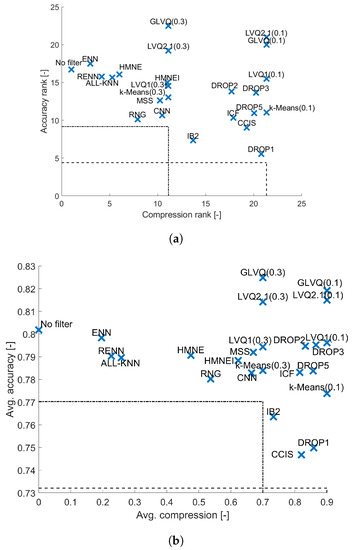
Figure 4.
Results obtained for 1-NN classifier. (a) Average performance ranks. (b) Average performance.
4.2. kNN
In the case of kNN similarly the best results are obtained for GLVQ and LVQ2.1 (see Figure 5), but they do not differ significantly from the results obtained by kNN with optimally tuned k parameter. All other filters appears to decrease classification accuracy. Also noticeable is the fact that now IB2 appears to be dominated by the random sampling, as well as All-kNN and Drop1 in terms of average accuracy.
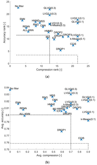
Figure 5.
Results obtained for kNN classifier. (a) Average performance ranks (b) Average performance.
4.3. Naive Bayes
The results obtained for Naive Bayes are shown in Figure 6. There is no significant difference between the accuracy obtained for the two random sampling methods (one with compression and the second with compression ). The difference between these two in terms of ranks is less than 1. For Naive Bayes the highest accuracy is obtained by the ENN and RENN, for which the comparison to the reference method is statistically significantly different. Also All-kNN is very high, but the Wilcoxon test does not indicate significant statistical difference. That is reasonable because noise filters remove the noise samples which affects the probability distributions estimated by the Naive Bayes classifier. Here the LVQ family, especially the GLVQ(0.3) algorithm, displays similar performance to noise filters, but with the compression reaching , unfortunately the difference to the reference method is not significant. Also other prototype construction methods like other LVQ algorithms as well as k-Means clustering method do not show significant differences. From the group of evaluated methods almost all instance selection algorithms are dominated by the random sampling so all these methods can be considered as unhelpful.
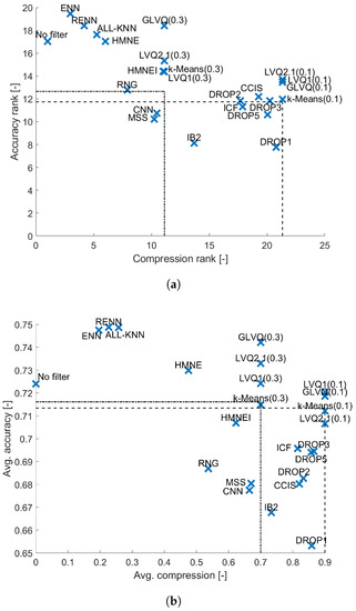
Figure 6.
Results obtained for Naive Bayes classifier. (a) Average performance ranks. (b) Average performance.
4.4. GLM
The linear model without instance selection provided the highest accuracy, as shown in Figure 7 and by applying any data filter we may expect a drop in accuracy. The highest accuracy using filters is obtained for ENN and HMN-E and for larger compression methods with LVQ1, GLVQ and Drop3, but all these results are statistically significantly different. It is important to mention that the linear model can be efficiently implemented, so the data filters are not necessarily required, because they extend the computation time. For GLM nine models are dominated by random sampling, these are Drop1, Drop2, Drop5, ICF, CCIS, CNN, MSS, HMN-EI and All-kNN and many are close to the border like GLVQ, LVQ2.1 or k-Means, so in general it is not recommended to perform any data filtering for the GLM model.
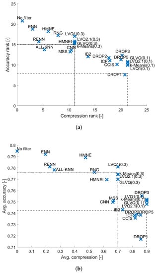
Figure 7.
Results obtained for GLM classifier. (a) Average performance ranks. (b) Average performance.
4.5. C4.5 Decision Tree
In the case of C4.5 decision tree (see Figure 8) it could be expected that any dataset reduction may result in the drop of accuracy. This is due to the quality of estimated statistics which are determined when selecting the split nodes. As a result the majority of data filters are dominated by random sampling. Only noise filters allows to achieve the accuracy comparable to the one obtained by the reference method, moreover the results for ENN and All-kNN are not statistically significantly different. This is due to the fact that noise filters have very low compression, but also regularizing the decision boundary by eliminating the noise samples can have positive influence on the estimated measures of decision tree nodes quality. For the condensation methods only Drop3, Drop2 and ICF achieve results not dominated by random sampling.
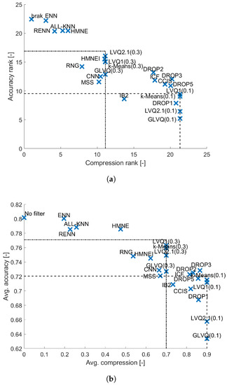
Figure 8.
Results obtained for C4.5 classifier. (a) Average performance ranks. (b) Average performance.
4.6. Random Forest
Random Forest is a classifier which is also based on the decision tree but thanks to the properties of collective decision making it can overcome some of its weaknesses. As shown in Figure 9 only ENN achieves comparable accuracy to the one obtained with entire training set. However, almost all data filtering methods especially instance selection methods are better than random sampling (except HMN-EI and All-kNN which lie on the border), and almost all prototype construction methods (except LVQ1) lie on the bounds defined by random sampling. Note that here all methods are statistically significantly different from the reference method, that is worse than the reference solution.
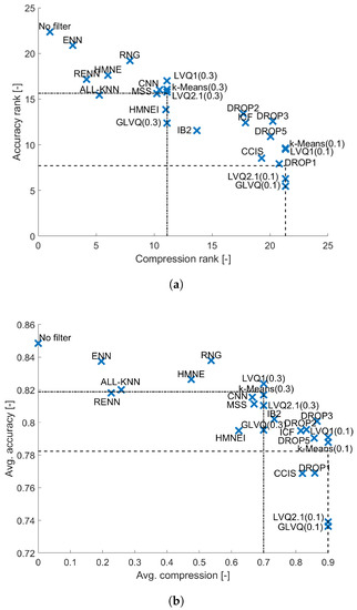
Figure 9.
Results obtained for Random Forest classifier. (a) Average performance ranks. (b) Average performance.
4.7. SVM
The final of the evaluated classifiers is SVM which is one of the most robust classifiers (similarly to Random Forest). The results presented in Figure 10 indicate that all the examined instance selection methods lead to decrease in prediction accuracy. Moreover, for the compression level of up to the top data filters are ENN, HMN-E, RNGE, CNN, k-Means and LVQ1, which on average share similar accuracy rank. Further increase in compression leads to significant drop in accuracy rank, so the best methods with compression equal like k-Means and LVQ1 have accuracy rank almost 8 points lower. For SVM only RENN, All-kNN and HMN-EI (which all belong to the noise filters) are outperformed by random sampling. The reason fo that are the figh tolerance on noise in the data that can be controlled by C parameter in SVM.
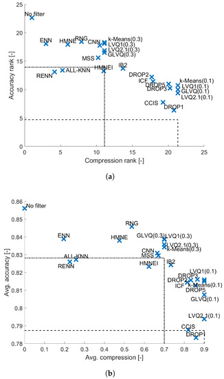
Figure 10.
Results obtained for SVMclassifier. (a) Average performance ranks. (b) Average performance.
5. Conclusions
In the article we investigated the performance of the popular classical instance selection and prototype generation methods in terms of the obtained compression of the data set and their influence on the performance of various classifiers. To summarize the obtained results we averaged them for each data filtering method over all classifiers. This allowed us to compare all the evaluated data filters. The results are presented in Figure 11. The red line in the plots indicate the methods which belong to the Pareto front, for example, these ones which are not dominated by the other methods. The following methods belong to the front: ENN, HMN-E, GLVQ(0.3), LVQ2.1(0.3), HMN-EI, Drop2, Drop3 and LVQ2.1(0.1). Some other methods like k-Means(0.3) and LVQ1 can be considered as the top ones because they lie very close to the Pareto front. From the top methods two algorithms provide compression less than , these are ENN and HMN-E. These methods should be considered only when the compression is not the primary need.
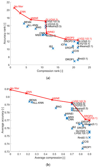
Figure 11.
Average results over all evaluated classifiers. Red line represents Pareto front. (a) Average performance ranks. (b) Average performance.
In theory, as indicated in the beginning of this article, the goal of data filtering methods is to keep the estimated conditional probabilities unchanged before and after data filtering so that the , but in reality each of these classifiers has its own probability estimation technique. So the one used by the decision trees which is based on the instance frequency calculation within the bin, do not match with the one of the nearest neighbor classifier. Moreover, SVM and Random Forest are more robust than kNN so they can better deal with the noisy samples than the data filters which internally use kNN to assess training instances.
The obtained results indicate that the size of the dataset matters. In general applying any of the examined data filters result in the decrease in accuracy, and a huge drop in prediction performance can be observed between compression 70% and 90%, so that the compression 70% can be considered as a kind of threshold below which we should not compress the dataset. Although, we also observed, that for bigger datasets instance selection methods proved more efficient allowing for higher compression. Interestingly, on average the prediction performance slowly drops even for the noise filters. The exception are 1-NN and Naive Bayes classifiers where some of the tested instance filtering methods (in particular ENN and the LVQ family) allowed to increase the accuracy. For the kNN with tuned k the accuracy may remain unchanged, so the benefit is the execution time of the prediction phase, which requires fewer distance calculations to make the decision.
The observed phenomenon can be interpreted taking into account that all of the tested instance selection methods were developed to work with kNN. As it was indicated in Section 2 instance selection methods can be considered wrappers for the kNN classifier, while for the remaining classifiers they work as filters. Some authors design specific algorithms for particular classifiers. The examples are the works of Kawulok and Nalepa who developed memetic [37] and genetic [38] algorithms for SVM, also de Mello and others developed an algorithm dedicated for the SVM [39]. In [7] we developed generalized CNN and ENN algorithms which work as wrappers in particular with MLP network. But these methods are strictly designed for given classifiers and can not be generalized so they were not considered in this research.
In the literature some authors use instance selection methods for balancing the data distribution of unbalanced classification problems [40]. In this scenario instance selection methods are applied to down-sample the majority class, and the minority classes remain unchanged, but this aspect was not considered in our study. Also the problem of applying instance selection methods to other tasks such as regression [41], multi-label learning [42] or stream mining [43] was not covered and requires further studies. Another open question which remains is deeper analysis of why particular of evaluated methods are better than the competitors. This requires independent analysis on lower number of methods and remains for future investigation.
In summery, when considering the use of initial data filtering for training set reduction one should consider GLVQ, LVQ2.1 and in the case where it is needed to use the original training samples and not newly constructed prototypes one should consider Drop2 Drop3 from the set of evaluated methods. These methods provide significant dataset size reduction and in general allow to obtain the higher prediction accuracy in comparison to the other methods with similar compression, but by applying them we should expect a drop in prediction accuracy for classifiers other than kNN.
Author Contributions
Conceptualization, M.B.; methodology, M.B.; software, M.B.; validation, M.B., M.Kordos.; formal analysis, M.B.; investigation, M.B. and M.K.; resources, M.B.; data curation, M.B.; writing—original draft preparation, M.B.; writing—review and editing, M.B., M.K.; visualization, M.B. and M.K.; supervision, M.B.; project administration, M.B.; funding acquisition, M.B. All authors have read and agreed to the published version of the manuscript.
Funding
The APC was funded by Silesian University of Technology BK-204/2020/RM4
Conflicts of Interest
The authors declare no conflict of interest.
Abbreviations
The following abbreviations are used in this manuscript:
| SVM | Support Vector Machine |
| Random Forest | Random Forest |
| kNN | k-Nearest Neighbor |
| 1-NN | 1-Nearest Neighbor |
| C4.5 | C4.5 decision tree |
| GLM | Generalized Linear Model |
| Naive Bayes | Naive Bayes |
| MLP | Multi Layer Perceptron |
| Linear Regression | Linear Regression |
| ENN | Edited Nearest Neighbor Rule |
| CNN | Condenced Nearest Neighbor Rule |
| RENN | Repeated ENN |
| ICF | Iterative Case Filtering |
| IB3 | Instance Based Learining version 3 |
| IB2 | Instance Based Learining version 2 |
| GGE | Gabriel Graph Editing |
| RNGE | Relative Neighbor Graph Editing |
| MSS | Modified Selective Subset Selection |
| LVQ | Learning Vector Quantization |
| LVQ1 | Learning Vector Quantization version 1 |
| LVQ2 | Learning Vector Quantization version 2 |
| LVQ2.1 | Learning Vector Quantization version 2.1 |
| LVQ3 | Learning Vector Quantization version 3 |
| OLVQ1 | Optimized Learning Vector Quantization |
| GLVQ | Generalized Learning Vector Quantization |
| SNG | Suppervised Neural Gas |
| CCIS | Class Conditional Instance Selection |
| HMN | Hit Miss Network |
| HMN-C | Hit Miss Network Condensation |
| HMN-E | Hit Miss Network Editing |
| HMN-EI | Hit Miss Network Iterative Editing |
| RNN | Reduced Nearest Neighbor Rule |
References
- Blachnik, M. Reducing Time Complexity of SVM Model by LVQ Data Compression. In Artificial Intelligence and Soft Computing; LNCS 9119; Springer: Berlin, Germany, 2015; pp. 687–695. [Google Scholar]
- Duch, W.; Grudziński, K. Prototype based rules—New way to understand the data. In Proceedings of the IEEE International Joint Conference on Neural Networks, Washington, DC, USA, 15 July 2001; pp. 1858–1863. [Google Scholar]
- Blachnik, M.; Duch, W. LVQ algorithm with instance weighting for generation of prototype-based rules. Neural Networks 2011, 24, 824–830. [Google Scholar] [CrossRef]
- Kraskov, A.; Stögbauer, H.; Grassberger, P. Estimating mutual information. Phys. Rev. E 2004, 69, 066138. [Google Scholar] [CrossRef]
- García, S.; Luengo, J.; Herrera, F. Tutorial on practical tips of the most influential data preprocessing algorithms in data mining. Knowl. Based Syst. 2016, 98, 1–29. [Google Scholar] [CrossRef]
- Blachnik, M.; Kordos, M.; Wieczorek, T.; Golak, S. Selecting Representative Prototypes for Prediction the Oxygen Activity in Electric Arc Furnace. LNCS 2012, 7268, 539–547. [Google Scholar]
- Kordos, M.; Blachnik, M.; Białka, S. Instance Selection in Logical Rule Extraction for Regression Problems. LNAI 2013, 7895, 167–175. [Google Scholar]
- Abdulali, A.; Hassan, W.; Jeon, S. Stimuli-magnitude-adaptive sample selection for data-driven haptic modeling. Entropy 2016, 18, 222. [Google Scholar] [CrossRef]
- Blachnik, M. Instance Selection for Classifier Performance Estimation in Meta Learning. Entropy 2017, 19, 583. [Google Scholar] [CrossRef]
- Grochowski, M.; Jankowski, N. Comparison of Instance Selection Algorithms. II. Results and Comments. LNCS 2004, 3070, 580–585. [Google Scholar]
- Borovicka, T.; Jirina, M., Jr.; Kordik, P.; Jirina, M. Selecting representative data sets. In Advances in Data Mining Knowledge Discovery and Applications; IntechOpen: London, UK, 2012. [Google Scholar]
- Blachnik, M.; Duch, W. Prototype-based threshold rules. Lect. Notes Comput. Sci. 2006, 4234, 1028–1037. [Google Scholar]
- García, S.; Derrac, J.; Cano, J.R.; Herrera, F. Prototype selection for nearest neighbor classification: Taxonomy and empirical study. IEEE Trans. Pattern Anal. Mach. Intell. 2012, 34, 417–435. [Google Scholar] [CrossRef]
- Triguero, I.; Derrac, J.; Garcia, S.; Herrera, F. A taxonomy and experimental study on prototype generation for nearest neighbor classification. IEEE Trans. Syst. Man, Cybern. 2012, 42, 86–100. [Google Scholar] [CrossRef]
- Hart, P. The condensed nearest neighbor rule. IEEE Trans. Inf. Theory 1968, 16, 515–516. [Google Scholar] [CrossRef]
- Aha, D.; Kibler, D.; Albert, M. Instance-Based Learning Algorithms. Mach. Learn. 1991, 6, 37–66. [Google Scholar] [CrossRef]
- Marchiori, E. Hit miss networks with applications to instance selection. J. Mach. Learn. Res. 2008, 9, 997–1017. [Google Scholar]
- Barandela, R.; Ferri, F.J.; Sánchez, J.S. Decision boundary preserving prototype selection for nearest neighbor classification. Int. J. Pattern Recognit. Artif. Intell. 2005, 19, 787–806. [Google Scholar] [CrossRef]
- Wilson, D.; Martinez, T. Reduction techniques for instance-based learning algorithms. Mach. Learn. 2000, 38, 257–268. [Google Scholar] [CrossRef]
- Tomek, I. An experiment with the edited nearest-neighbor rule. IEEE Trans. Syst. Man Cybern. 1976, 6, 448–452. [Google Scholar]
- Wilson, D. Assymptotic properties of nearest neighbour rules using edited data. IEEE Trans. Syst. Man Cybern. 1972, SMC-2, 408–421. [Google Scholar] [CrossRef]
- Sánchez, J.S.; Pla, F.; Ferri, F.J. Prototype selection for the nearest neighbour rule through proximity graphs. Pattern Recognit. Lett. 1997, 18, 507–513. [Google Scholar] [CrossRef]
- Brighton, H.; Mellish, C. Advances in instance selection for instance-based learning algorithms. Data Min. Knowl. Discov. 2002, 6, 153–172. [Google Scholar] [CrossRef]
- Marchiori, E. Class conditional nearest neighbor for large margin instance selection. IEEE Trans. Pattern Anal. Mach. Intell. 2010, 32, 364–370. [Google Scholar] [CrossRef] [PubMed]
- Nova, D.; Estévez, P.A. A review of learning vector quantization classifiers. Neural Comput. Appl. 2014, 25, 511–524. [Google Scholar] [CrossRef]
- Blachnik, M.; Kordos, M. Simplifying SVM with Weighted LVQ Algorithm. LNCS 2011, 6936, 212–219. [Google Scholar]
- Kordos, M.; Blachnik, M. Instance Selection with Neural Networks for Regression Problems. LNCS 2012, 7553, 263–270. [Google Scholar]
- Arnaiz-González, Á.; Díez-Pastor, J.F.; Rodríguez, J.J.; García-Osorio, C. Instance selection of linear complexity for big data. Knowl.-Based Syst. 2016, 107, 83–95. [Google Scholar] [CrossRef]
- De Haro-García, A.; Cerruela-García, G.; García-Pedrajas, N. Instance selection based on boosting for instance-based learners. Pattern Recognit. 2019, 96, 106959. [Google Scholar] [CrossRef]
- Arnaiz-González, Á.; González-Rogel, A.; Díez-Pastor, J.F.; López-Nozal, C. MR-DIS: Democratic instance selection for big data by MapReduce. Prog. Artif. Intell. 2017, 6, 211–219. [Google Scholar] [CrossRef]
- Blachnik, M.; Duch, W.; Wieczorek, T. Selection of prototypes rules – context searching via clustering. LNCS 2006, 4029, 573–582. [Google Scholar]
- Kuncheva, L.; Bezdek, J. Presupervised and postsupervised prototype classifier design. IEEE Trans. Neural Networks 1999, 10, 1142–1152. [Google Scholar] [CrossRef]
- Herrera, F. KEEL, Knowledge Extraction based on Evolutionary Learning. Spanish National Projects TIC2002-04036-C05, TIN2005-08386-C05 and TIN2008-06681-C06. 2005. Available online: http://www.keel.es (accessed on 1 May 2020).
- Blachnik, M.; Kordos, M. Information Selection and Data Compression RapidMiner Library. In Machine Intelligence and Big Data in Industry; Springer: Berlin, Germany, 2016; pp. 135–145. [Google Scholar]
- Alcalá-Fdez, J.; Fernández, A.; Luengo, J.; Derrac, J.; García, S.; Sanchez, L.; Herrera, F. KEEL data-mining software tool: Data set repository, integration of algorithms and experimental analysis framework. J. Mult. Valued Log. Soft Comput. 2011, 17, 255–287. [Google Scholar]
- Demšar, J. Statistical comparisons of classifiers over multiple data sets. J. Mach. Learn. Res. 2006, 7, 1–30. [Google Scholar]
- Nalepa, J.; Kawulok, M. Adaptive memetic algorithm enhanced with data geometry analysis to select training data for SVMs. Neurocomputing 2016, 185, 113–132. [Google Scholar] [CrossRef]
- Kawulok, M.; Nalepa, J. Support vector machines training data selection using a genetic algorithm. In Joint IAPR International Workshops on Statistical Techniques in Pattern Recognition (SPR) and Structural and Syntactic Pattern Recognition (SSPR); Springer: Berlin, Germany, 2012; pp. 557–565. [Google Scholar]
- De Mello, A.R.; Stemmer, M.R.; Barbosa, F.G.O. Support vector candidates selection via Delaunay graph and convex-hull for large and high-dimensional datasets. Pattern Recognit. Lett. 2018, 116, 43–49. [Google Scholar] [CrossRef]
- Devi, D.; Purkayastha, B. Redundancy-driven modified Tomek-link based undersampling: A solution to class imbalance. Pattern Recognit. Lett. 2017, 93, 3–12. [Google Scholar] [CrossRef]
- Arnaiz-González, Á.; Díez-Pastor, J.; Rodríguez, J.J.; García-Osorio, C.I. Instance selection for regression by discretization. Expert Syst. Appl. 2016, 54, 340–350. [Google Scholar] [CrossRef]
- Kordos, M.; Arnaiz-González, Á.; García-Osorio, C. Evolutionary prototype selection for multi-output regression. Neurocomputing 2019, 358, 309–320. [Google Scholar] [CrossRef]
- Gunn, I.A.; Arnaiz-González, Á.; Kuncheva, L.I. A Taxonomic Look at Instance-based Stream Classifiers. Neurocomputing 2018, 286, 167–178. [Google Scholar] [CrossRef]
© 2020 by the authors. Licensee MDPI, Basel, Switzerland. This article is an open access article distributed under the terms and conditions of the Creative Commons Attribution (CC BY) license (http://creativecommons.org/licenses/by/4.0/).