Process Monitoring of Antisolvent Based Crystallization in Low Conductivity Solutions Using Electrical Impedance Spectroscopy and 2-D Electrical Resistance Tomography

Abstract

Industrial process monitoring is an important field of research where different chemical processes are monitored and controlled. In this work, electrical impedance spectroscopy (EIS) was used to analyze antisolvent based crystallization of sucrose solutions. The impedance and phase spectra were recorded for four known sucrose concentrations in water, and for each case, four predetermined amounts of ethanol were added. As a result, sixteen different solutions involving sucrose solutions of different concentrations and ethanol to water ratios were analyzed. Significant differences were observed in the magnitude and phase spectra of the solutions in the frequency range of 50 kHz to 300 kHz. The experimentally obtained data from the EIS were converted into frequency response models. Three continuous-time transfer function models of the first-order, second-order, and a second-order with a zero were estimated and compared. In addition, a 2-D electrical resistance tomography (ERT) system with a low conductivity sensor unit was designed and tested with demineralized water, tap water and industrial food grade saturated sucrose solution. Non-conducting phantom and sugar crystals were observed within the saturated sucrose solution using the Bayesian reconstruction algorithm. These demonstrations have the potential to be developed into a multi-frequency ERT systems for monitoring the distribution of the crystals in the reactor. The EIS modality can be a complementary process analytical technology (PAT) tool indicating supersaturation status and provide quality assurance.

1. Introduction

Industrial process monitoring and automation is an important field of applied research, which involves development and implementation of novel process analytical technologies (PAT) in a variety of industries such as food, pharmaceutical, specialty chemicals, and petroleum. Monitoring and control of processes at the industrial scale are inherently challenging due to the scale, sensitivity, and complexity of the manufacturing units. A large number of PAT instrumentation, sensors and measurement techniques [1,2] have recently emerged such as attenuated total reflectance Fourier-transform infrared (ATR-FTIR), focused beam reflectance measurement (FBRM), Raman spectroscopy, particle vision and measurement (PVM) [3], electrical capacitance tomography [4,5], electrical resistance tomography [6] and ultrasound tomography [7,8]. Depending on the characteristics of the process, the properties of the liquid or solid phase, and the type of measurement technique (i.e. in situ, online, or offline), different sensor technologies are adopted. Additionally, different new data acquisition and processing methods have been developed to speed up computations or improve measuring accuracy [9], for example, parallel computing, artificial neural networks [10], and machine learning [11].

PAT is particularly important in crystallization processes for the production of value-added materials. In these processes, real-time monitoring can augment understanding of the fundamentals of the crystallization mechanisms (e.g., nucleation and growth), quantify the concentration evolution, and eventually control the crystal size distribution (CSD) [12]. Crystallization is an essential separation and purification technique in the industry that can be carried out in different ways. The main driving force of the process is the supersaturation of the solute [13,14].

In crystallization from solution, supersaturation could be generated by changing the solubility of the primary solvent through the addition of a second solvent–antisolvent. Crystallization occurs because the antisolvent reduces the solute solubility in the resulting mixed solvent. The antisolvent crystallization approach, which is usually performed in a semi-batch manner, is customary practice in pharmaceuticals, nutraceutical, and agrochemicals [15]. The antisolvent method is comparatively less energy demanding and can be carried out at ambient temperature conditions [16]. In addition, it has a more significant effect on the crystalline structure and morphology due to a profound change in solvent activity; thus, it has a potential for the production of highly purified solid materials [12].

Given the importance of antisolvent crystallization technique in industrial processes, a wide range of multidisciplinary studies have been conducted to increase the understanding of the kinetics of the process and to develop sensors and monitoring instrumentation. Ultrasonic power and offline measurements were used to control crystal size distribution during antisolvent crystallization of paracetamol [17], sodium chloride [18], and glycine [19], and combined cooling/antisolvent crystallization of acetylsalicylic acid in ethanol–water mixtures were monitored using ATR-FTIR and FBRM spectroscopy [20]. The antisolvent crystallization process of sodium benzoate was monitored with a combination of in situ FBRM and ultraviolet–visible spectroscopy sensors [21].

Amongst the many different approaches for process monitoring, electrical impedance spectroscopy (EIS) is a well-known method that has been extensively used in various manufacturing industries such as pulp and paper [22], bio-analytical applications [23,24,25], and food characterization [26,27]. Impedance spectroscopic measurements can be performed quickly and are economically cheaper. Wideband impedance spectroscopic measurements can pave the way towards process evaluation in a multi-parameter acquisition system [28]. Therefore, it is required to investigate the feasibility of EIS as an online monitoring tool in crystallization processes [29].

In global food processing industries, sucrose (C₁₂H₂₂O₁₁) production has a significant importance, and crystallization plays a fundamental role in its manufacturing process. Applications of process monitoring techniques in sucrose crystallization and manufacturing have been seldom reported in the literature and works have been limited to cooling and evaporative crystallization and concentration measurements [30]. For instance, applications of EIS [31] and image acquisition by high-speed camera [32] have been successfully demonstrated during cooling crystallization of sucrose. Moreover, ultrasound computed tomography [7] systems have been used to evaluate concentration change in different sucrose solutions. Therefore, advancement in innovative monitoring methods and new crystallization techniques are critical to ensuring the improvement in final particle quality as well as intensifying the overall process in terms of energy and sustainability.

Hence, given the status quo of research and development both in antisolvent–based crystallization processes and PAT, applications of two different process monitoring techniques, namely, 1-D spectroscopy and 2-D electrical resistance tomography, have been proposed and investigated in this study. The aim of the work was to investigate the feasibility of both methods for crystallization process monitoring and control. Given the low conductivity of the sucrose solutions in the range of a few µS/cm [33], electrical resistance tomography (ERT) reconstructions become challenging due to the small changes in the resistances [34]. However, in the recent years, it has been demonstrated that the ERT can be successfully implemented with materials with low conductivity such as composite structures [35], graphene-based nano-composite films [36] and bone cement [37]. Herein, electrical properties of antisolvent crystallization in the ternary–sucrose–ethanol-water system were analysed by utilizing 1-D thin electrode impedance spectroscopy. The acquired experimental data was used to build a frequency response model in the form of a transfer function. Additionally, this study is further supplemented by 2-D visualization of the crystal distribution in low conductivity standard solutions of saturated sucrose via an in-house ERT unit. The results of EIS can be utilized in the further development of electrical resistance tomography to design a multispectral acquisition methodology [38,39], specifically for crystallization processes and for process control purposes.

This work has been done within the European Union Horizon 2020 TOMOCON project (Smart tomographic sensors for advanced industrial process control) [40]. The aim within the project is to create a multi-sensor network to monitor, visualize, and control the different industry-relevant cases, including batch crystallization processes.

2. Application of 1-D EIS and 2-D ERT as a PAT in Crystallization Processes

2.1. Application of Electrical Impedance Spectroscopy to the Crystallization Process

Impedance is dependent on the electrical conductivity of the solution. Electrical conductivity is calculated from the measurement of the corresponding material property such as resistance [41]. Fluid may have many dielectric mechanisms or polarization effects that contribute to its overall permittivity, such as ionic, dipolar, atomic, or electronic, depending on the frequency applied. Equation (1) gives the general Ohms law for calculating impedance Z and its dependence on the conductivity in phasor notation. Here sinusoidal signals at angular frequency ω are considered where V denotes the electric voltage phasor applied to the sensor (or sensing cell) and I the resulting electric current phasor. The impedance Z is a complex number and has two components, namely magnitude and phase, as given in Equation (2).

The equation of impedance in phasor form is

$$Z\left(\omega \right)=\frac{V\left(\omega \right)}{I\left(\omega \right)}=A\left(\omega \right)e^{j\phi \left(\omega \right)}$$

(1)

where A is the magnitude (impedance module) and φ is the phase of the evaluated impedance. As a complex quantity, the impedance can be expressed in the rectangular form as follows:

$$Z\left(\omega \right)=R\left(\omega \right)+jX\left(\omega \right)$$

(2)

where R is the resistance and X is the reactance of the evaluated impedance.

Impedance spectroscopy aims at measuring the impedances of the circuit, material, or any other component by applying the alternating voltage or current stimulus at different frequencies and measuring the response at these frequencies. These evaluations of the electrochemical behaviour of electrolyte materials are usually performed using two identical electrodes facing the sample inside a cylindrical cell [42]. In the field of electrochemical impedance spectroscopy [43], electrochemistry, instrumentation, process models, and statistical interpretation strategies have been discussed. Electrohydrodynamic impedances were evaluated to form a generalized transfer function of the non-electrical quantities. Multiple interpretation strategies for impedance representations and graphical methods were studied in detail.

Due to the advancement in modern impedance acquisition equipment and the development of signal processing capabilities, it is now faster to acquire and process the measurement data [44,45]. Several low and high accuracy methods for determining the conductivity of different types of liquids were studied along with fringe electric fields and interfacial effects due to the electrode area [46].

Impedance spectroscopy has been used from monitoring ions in aqueous solutions [47] to studying the cooling crystallization of ice [48]. In industrial processes, EIS has been used in batch crystallization processes as a 1-D PAT tool in order to characterize the amount of the precipitate in the mixture of the batch reactor. It is utilized to monitor the production and control of the quality of the product produced. Studies of the electrical behaviour of glucose using impedance spectroscopy [49] and impedance spectrum characterization after the addition of Na₂CO₃ have been performed [30]. The study of impedance signatures as a PAT tool for sucrose crystallization was recently done by [31]. During the crystallization of sugar using ethanol as an antisolvent, there is a mixture of three components in the solution. The impedances of all these three individual components are different. The study of the impedance signatures of sucrose solutions at various concentrations and at various ethanol to water ratios, and to model them into a transfer function is our interest of study in this module. Figure 1a shows the schematic of the setup made for the antisolvent crystallization. Figure 1b shows the sucrose–water phase equilibrium.

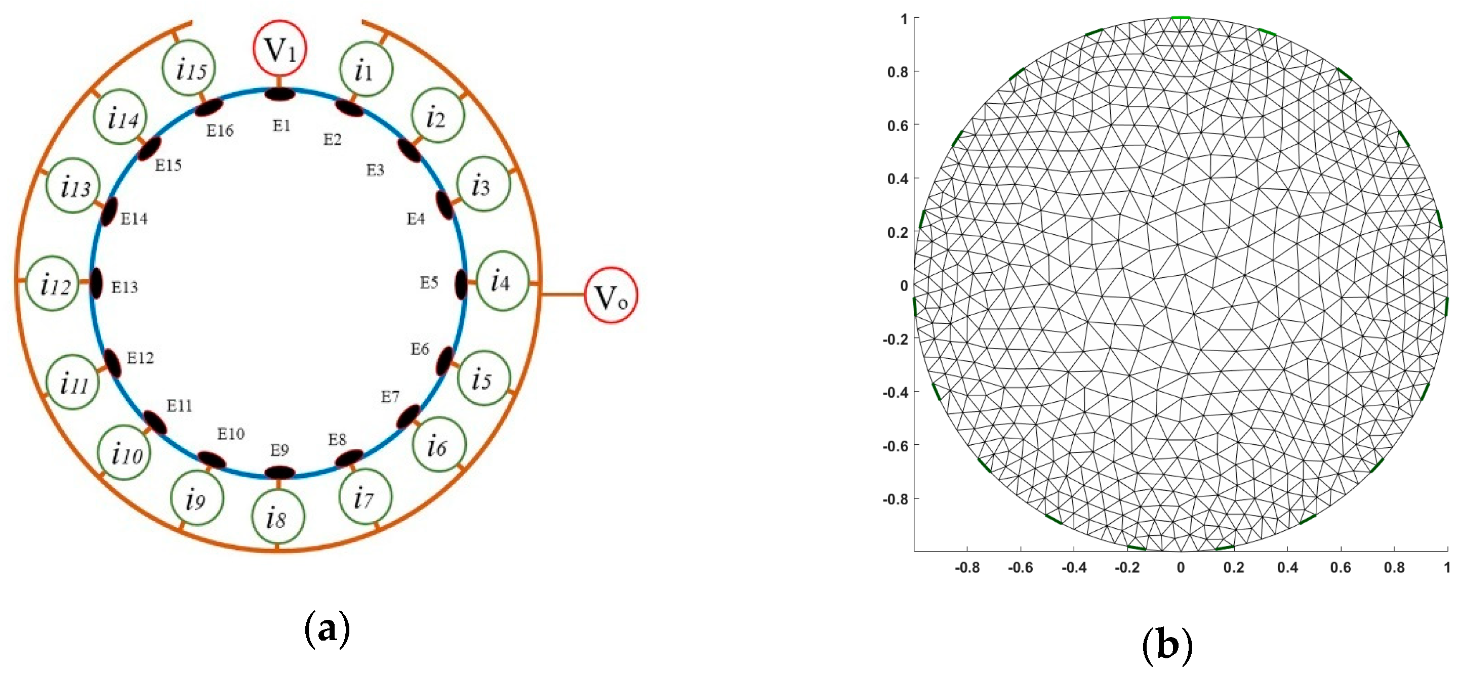
2.2. Application of a Voltage Injected–Current Detected (V–C) Based Low Conductivity Sensitive Electrical Resistance Tomography (ERT)

Although the EIS provides fast acquisition of data, this information is obtained in one dimension. This presents limitations for locating the crystal density distribution inside a reactor. Electrical resistance tomography is an imaging modality to visualize the binary or ternary phase flows and mixing in reactors based on the conductivity distribution. The conductivity distribution is visualized using electrical voltage or current measurements acquired from the boundary of the object. The electrical conductivity σ and electrical potential distribution Φ; are related to Maxwell’s equation in the sensing field Ω. Assuming a source-free region, in the case of ERT it can be simplified in the form of Equation (3) [51].

$$\nabla \left(\mathsf{\sigma }\nabla \Phi \right)=0 \mathrm{in} \mathsf{\Omega }$$

(3)

The forward problem is shown in Equation (4), where potential differences V between the electrode pair of a given injection is evaluated using the knowledge of σ. Usually, the finite element method (FEM) is used to govern Equation (3), to compute the numerical solution [51,52].

$$V=F\left(\mathsf{\sigma }\right)$$

(4)

In the inverse problem, the Jacobian matrix J is evaluated using current I in Equation (6), where the conductivity distribution σ is considered as piecewise constant and is expressed as in Equation (5) [53].

$$\mathsf{\sigma }={\displaystyle \sum }_{\mathrm{n}=1}^{\mathrm{N}}{\mathsf{\sigma }}_{\mathrm{n}}{\mathrm{X}}_{\mathrm{n}},$$

(5)

where X_n is the characteristic function, and X_n = 1 in the n^th element, and Ω_n and X_n = 0 otherwise.

$$\mathrm{J}=\frac{\partial I}{\partial {\mathsf{\sigma }}_n}$$

(6)

Novel reconstruction methods based on apriori information were developed by Vaukonen [54]. Various algorithms for ERT reconstruction have been discussed and reviewed in [55,56]. Image reconstructions using voltage-current methods were discussed in [53]. The ERT reconstruction methods involve deterministic and probabilistic approaches amongst others. Bayesian reconstruction is a probabilistic method where the regularization technique is connected to the covariance of the prior density, which is different from the regularization practices involving a regularization parameter. Probabilistic methods can be used even in the case of systems which do not have probabilistic behaviour. In these types of methods, the problems are formulated based on the probability theory. All the probability densities are considered as continuous. The joint density of the random vector x = (x₁,…x_N)^T is p(x). The joint density of the components of two random vectors x and y are denoted by p(x,y). The cross-covariance of x and y is defined as [54];

$$C_{xy}=E\left\{x{x}^T\right\}-{\mathsf{\eta }}_x{\mathsf{\eta }}_y^T$$

(7)

where, $E\left\{x{x}^T\right\}$ is the correlation matrix of random vector x and ${\eta }_x$ is the mean or expected value given by;

$${\mathsf{\eta }}_x={{\displaystyle \int }}_{-\infty }^{\infty }xp\left(x\right)dx$$

(8)

The conditional density of x given y is defined as;

$$p\left(x|y\right)=\frac{p\left(x,y\right)}{p\left(y\right)}$$

(9)

Whenever p(y) ≠ 0 and $p\left(x|y\right)$ = 0 otherwise. Clearly, it is also;

$$p\left(y|x\right)=\frac{p\left(x,y\right)}{p\left(x\right)}$$

(10)

Which helps in arriving at the Baye’s theorem which is given as;

$$p\left(x|y\right)p\left(y\right)=p\left(y|x\right)p\left(x\right)$$

(11)

Mathematical models for ERT and models for forward and inverse problem using Bayesian theorems along with a comparison of simulated and experimental data were performed by [51]. In this work, the commercially available software solutions from Rocsole Inc. was used to implement Bayesian reconstruction.

To complement the PAT evaluations in low conductivity ternary solutions, the low conductivity ERT monitoring data acquisition and sensor was designed and tested. The ERT sensor was placed at the circumference of a reactor. There are two types of ERT systems, namely current–voltage (C–V) based systems and voltage–current (V–C) based systems [53]. This classification is based upon the excitation electrode (source electrode) and the sensing electrode (sink electrode) configuration. In a C–V based system, the current is injected through the source and the voltages are measured at the sink electrodes, whereas in a V–C based system a voltage is injected through the source electrode and the currents are measured at the sink electrodes. In this work, a V–C based ERT was utilized. The device used step voltage interrogation at 156 KHz. Figure 2a shows the schematic for the V–C based system. In a system with 16 electrodes, E1 to E16, V1 (E1 as the source electrode) is excited using voltage, and all the other electrodes i1-i15 (sink electrodes E2–E16) simultaneously acquire the currents. This process is repeated for all the other electrodes. Finally, this data is collated inside a matrix with 256 data points. An image is then reconstructed using a forward model and by solving the inverse imaging equation [53]. Figure 2b shows an FEM mesh generated using EIDORS software in MATLAB [57]. The model is a 2-D circ model generated using Distmesh [58] using the function mk_common_model within EIDORS.

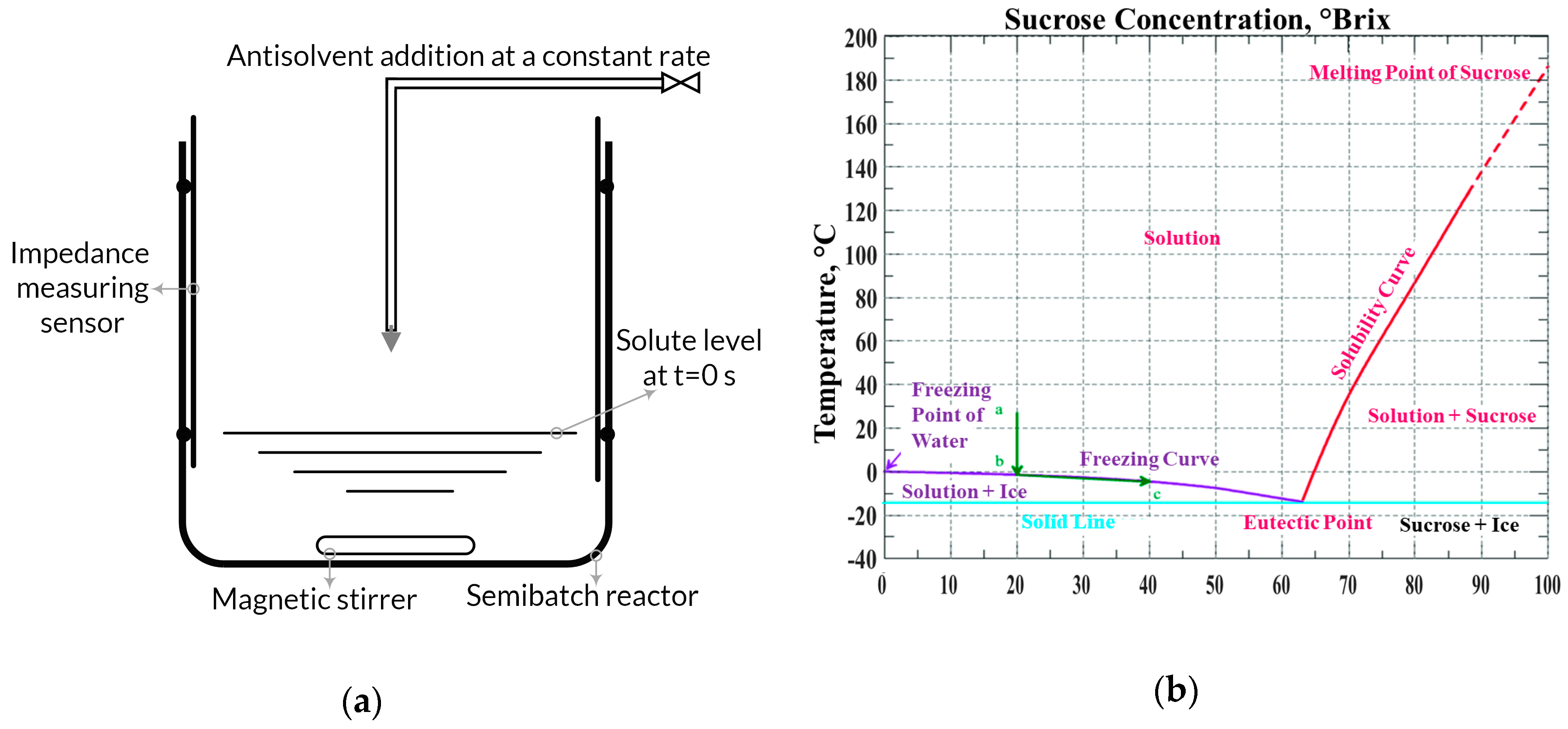
3. Experimental Setup, Materials, and Procedure

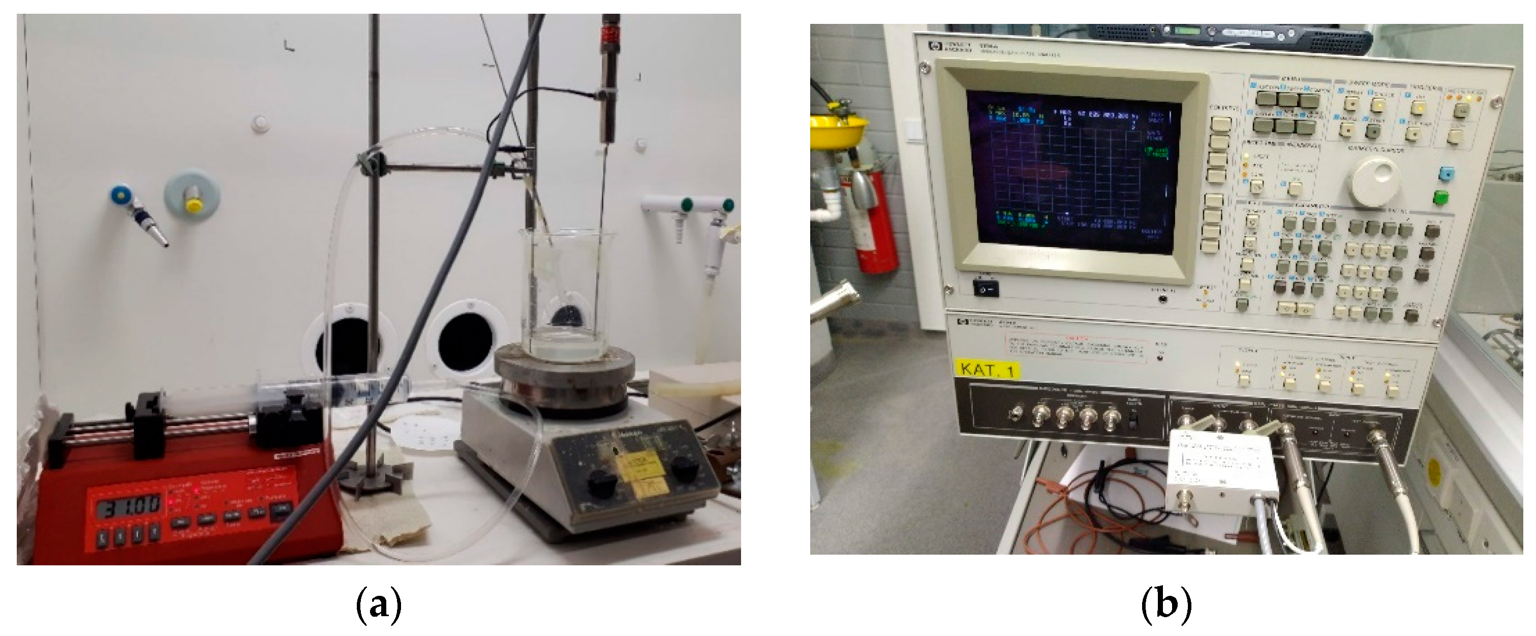
3.1. Experimental Apparatus Setup for EIS (Electrical Impedance Spectroscopy)

In this experiment, the impedance spectra were acquired using two thin steel electrodes. Several electrode geometries for the measurement of various electrical conductivity of liquids were discussed in [41]. The diameter and length of steel sensors were 1 mm and 150 mm, respectively. Crystallization experiments and the subsequent spectroscopic measurements were carried out in a small–scale laboratory crystallizer with a volume of 0.5 L equipped with a magnetic stirrer. The diameter of the glass vessel was 85 mm. Different concentrations of the fine sucrose (Nordic Sugar, Finland) solutions were prepared in deionized water. Technical grade ethanol (${\mathrm{C}}_2{\mathrm{H}}_5\mathrm{OH}$, purity $\ge$ 99.5 %), as the antisolvent, was used in different proportions.

Sixteen standard solutions of sucrose each with a volume of 100 mL and concentrations of 33 % w/w, 44 % w/w, 55 % w/w, and 66.67 % w/w (saturated sucrose solution at 20 °C) were prepared. As tabulated in

Table 1. The sucrose to ethanol ratio at the various concentration of the sucrose.

Solution Index	Effective Ethanol to Water Ratio	Different Concentrations of Sucrose Solutions (% w/w)	Sucrose Weight Percentage in 100 mL	Effective Sucrose/Ethanol Ratio in 100 mL Solution
1	0	33	33	-
2		44	44	-
3		55	55	-
4		66.67	66.67	-
5	0.33	33	19.87	1
6		4	24.85	1.33
7		55	29.25	1.66
8		66.67	33.16	2
9	0.66	33	16.58	0.5
10		44	20.95	0.66
11		55	24.88	0.83
12		66.67	28.44	1
13	0.99	33	14.22	0.33
14		44	18.10	0.44
15		55	21.65	0.55
16		66.67	24.90	0.66

, the amount of ethanol was proportional to water so that the ethanol to water ratio of the solutions remained constant at 0, 0.33, 0.66, and 0.99, respectively. Four different volumes of ethanol equivalents of 0, 33, 66, and 99 g were added to each sucrose solution.

The addition of the antisolvent to the crystallizer was controlled by a peristaltic syringe pump (Cole–Parmer GmbH) with an accompanying tubing of 2 mm diameter. The addition rate of 5 mL/min and a constant mixing speed of 400 RPM was maintained during the experiments. For each semi-batch operation, a consistent amount of 100 mL solution was taken for the measurement. The effective sucrose to ethanol ratios are shown in Table 1. Figure 3a,b presents a photograph of the experimental setup and the impedance gain, and phase analyser (Hewlett Packard 419 A) used, respectively.

The overall spectra were recorded for the wideband frequency range of 10 Hz to 1 MHz. This was done in three parts with each part recording 400 equidistant frequency data points. The first part was from 10 Hz to 100 kHz, the second part was from 100 kHz to 300 kHz, and the last part was from 300 kHz to 1 MHz. A total of 1200 data points were acquired for every solution. In order to increase the reliability and repeatability of the results, each experiment was repeated for a total of 5 times and averaged values were used for further post-processing.

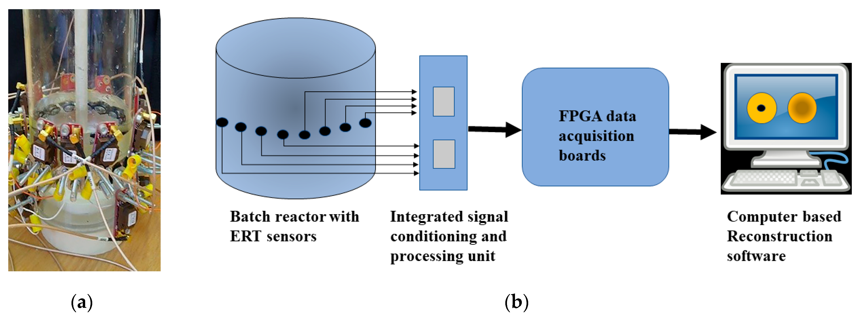
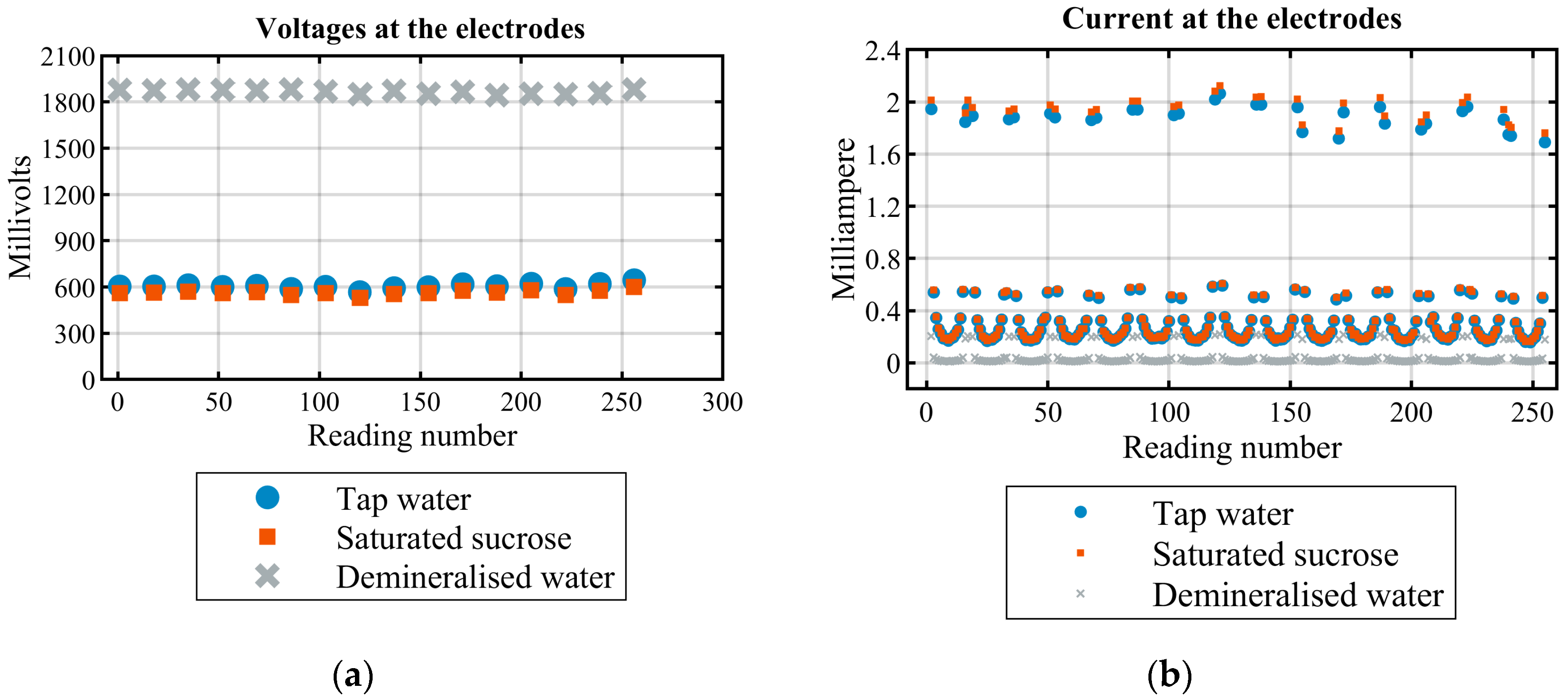
3.2. Experimental Apparatus Setup for ERT (Electrical Resistance Tomography)

A special ERT signal processing unit and data acquisition setup for evaluating low conductivity solutions was designed in cooperation with Rocsole Inc. In this module, the initial experimental studies utilizing the low conductivity liquid solutions of demineralized water, tap water, and industrial food grade saturated sucrose solution were performed. Blender v2.79 design software was used to design the phantoms with a 10 mm diameter. Ultimaker-3E 3-D printer was used to 3-D print manufacture these phantoms using the acrylonitrile butadiene styrene (ABS) material. A test demonstration was performed to visualize the density distribution for sucrose crystals within the industrial food grade saturated sucrose solution. Figure 4a shows the laboratory-based semi-batch reactor with ERT sensors mounted on it and Figure 4b displays the schematic for ERT data acquisition flow.

This reactor was made up of Plexiglas. The inner diameter of the reactor was 83 ± 0.3 mm. Sixteen circular-shaped sensors were placed along the perimeter at 5 cm from the bottom of the reactor. This allowed imaging of the planar region within the reactor. The distance between the sensors was 5.19 mm. The diameter of the sensor-head screw was 12 mm. The total surface area in contact with the medium for each sensor was 113.04 mm². The signal processing unit containing the amplifier and the noise removal electronics was mounted directly on the sensor tail. Using the MCX type of insulating co-axial cable, lossless transmission was achieved. The data acquisition system from Rocsole Inc. was utilized to acquire the ERT data. The Roc-GUI software interface was used to communicate between the ERT machine and the computer. The Bayesian reconstruction method was used to reconstruct the images [51].

The ERT was tested with all the three solutions in the V–C mode of operation. The voltage injected, and the current detected at each sensor were recorded. A phantom of 10 mm made up of ABS was placed at the centre of the beaker within an industrial food grade saturated sucrose solution, and an image was reconstructed. Various experiments using phantoms and sucrose solutions with relatively higher conductivity were done by [34]. The industrial food grade saturated sucrose solution was acquired from the Polish sugar company Polski Cukier. The cleaned, refined white sugar crystals (250 g) were also provided by the company. The beaker was filled with 500 mL of the industrial food grade saturated sucrose solution. The 250 g sugar crystals were added using a funnel towards the centre of the beaker at a rate of 8.3 g/s. Fast reconstructions based on the Bayesian method were applied using Roc-GUI to observe the density distribution of the crystals.

4. Results and Discussion

The results are divided into two parts. The results obtained using the EIS impedance spectroscopy module are discussed in Section 4.1. This includes the graphs plotted for the experimental data for the solutions and estimation of transfer functions using the MATLAB program. Section 4.2 shows the results obtained from the ERT module.

4.1. Results for EIS

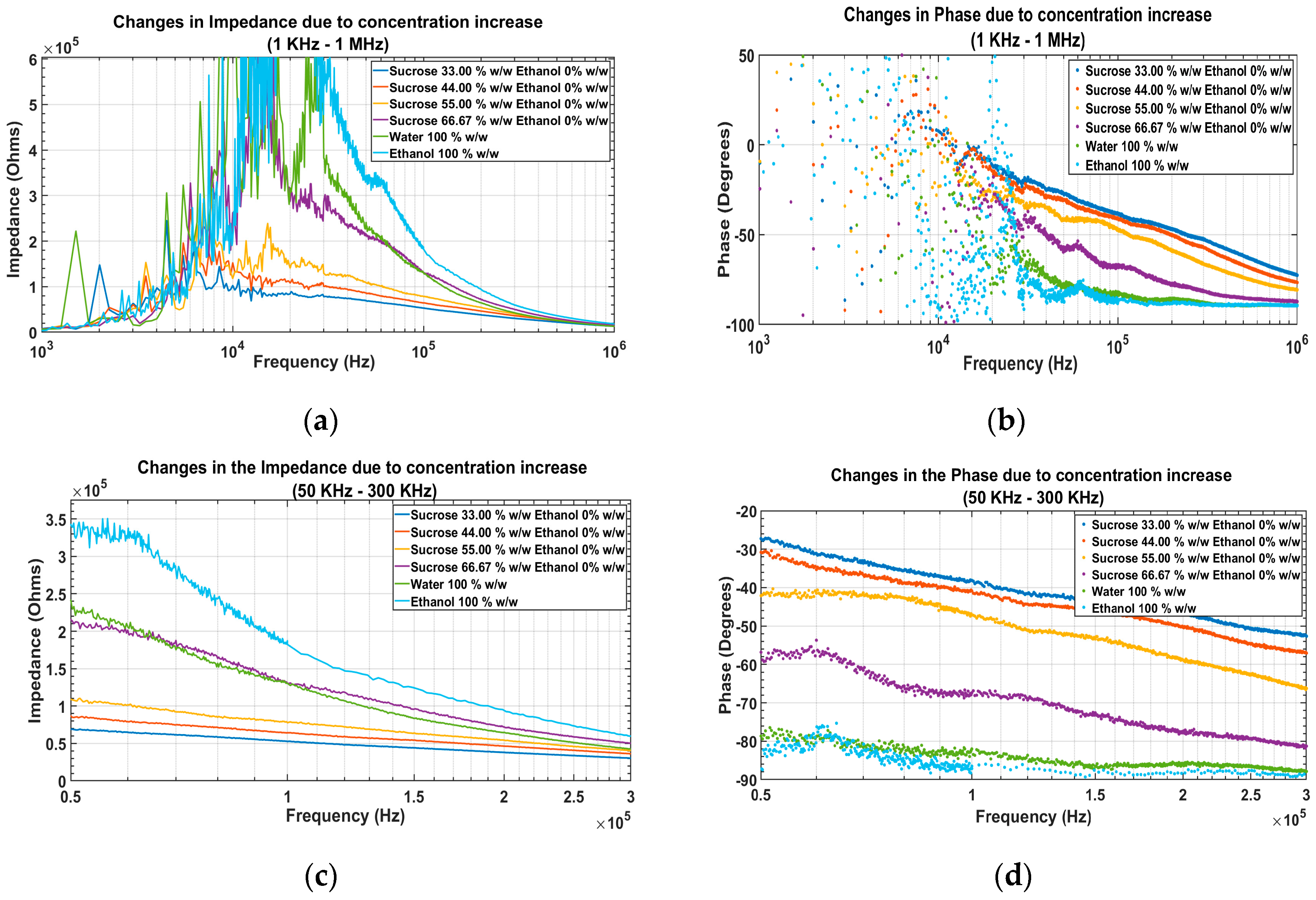
4.1.1. EIS of the Solutions before Adding Ethanol

Figure 5a displays the impedance magnitude of different concentrations of sucrose solutions, deionized water, and ethanol for the frequency range of 1 kHz to 1 MHz plotted on a logarithmic scale. Figure 5b shows the phase component of the spectrum in degrees of the solutions. It was observed that the impedance values at frequencies up to 50 kHz were much higher and unstable due to the electrode dimensions. Figure 5c shows the impedance magnitude in the frequency range of 50 kHz to 300 kHz. In this frequency range, a significant decrease in the impedance was observed. After 300 kHz, the impedance magnitude decrease was marginally discernible and conjoined together at higher frequencies. The phase angle, which was negative for all solutions, had a large standard deviation up to 50 kHz. From 50 kHz to 1 MHz, there was a decrease of a few degrees, as seen in Figure 5d.

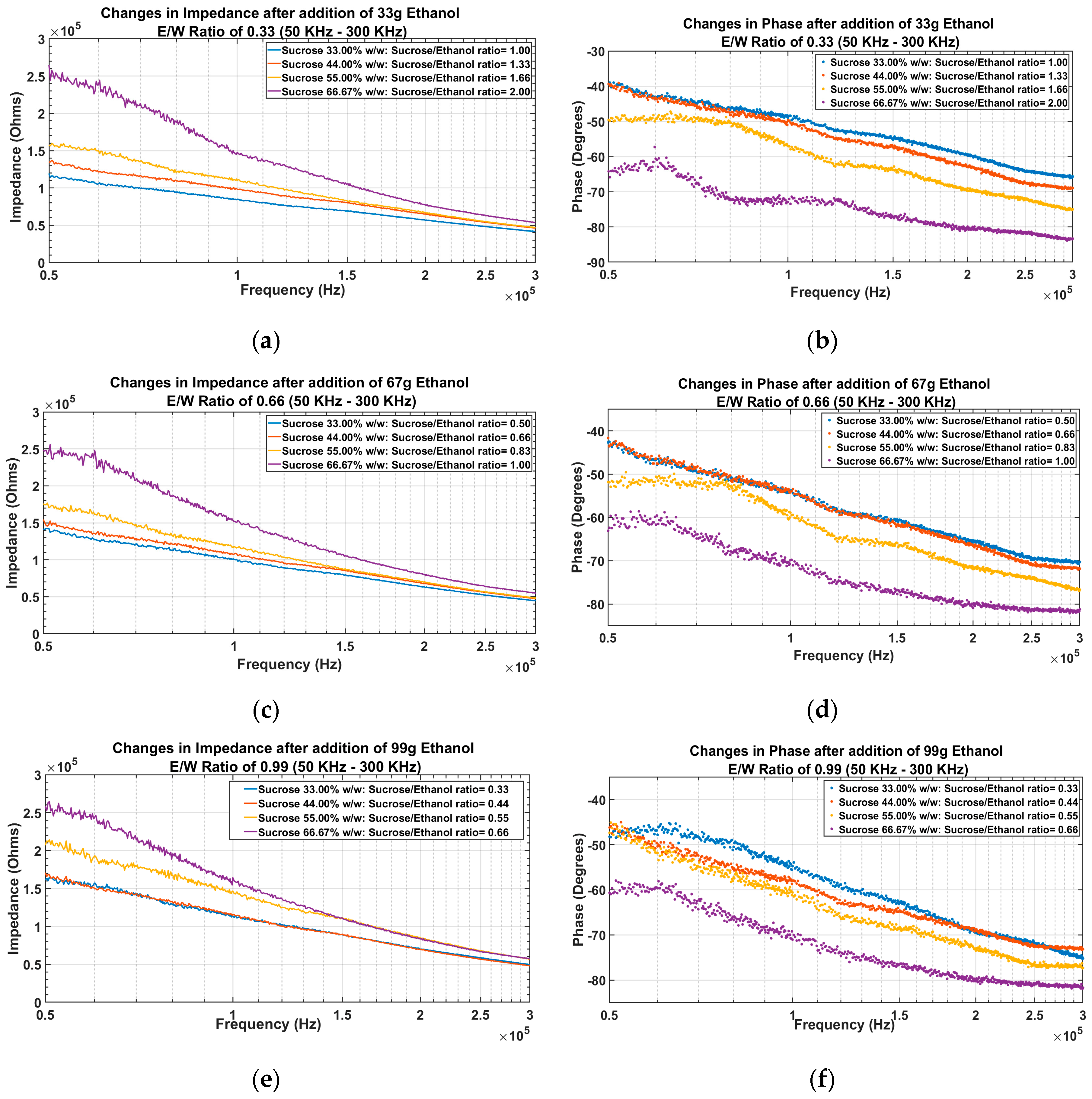
4.1.2. EIS of Solutions after Addition of Ethanol

Based on the results obtained in Section 4.1.1, the frequency range from 50 kHz to 300 kHz was analysed for the ternary solutions. The charts in Figure 6a–f shows the results from the experiment after the addition of ethanol. All the experimental results were acquired in the static solution of 100 mL. The three ethanol to water ratios of 0.33, 0.66, and 0.99 were analysed. The sucrose to ethanol ratio at 0.33 ranged from 1 to 2, at 0.66 it ranged from 0.5 to 1, and the sucrose to ethanol ratio at 0.99 ranged from 0.33 to 0.66. Figure 6a,c,e and Figure 6b,d,f show the changes in impedance and phase angles, respectively. Impedance magnitude, as the representation of the dielectric properties of the solution, increased, whereas the phase angle decreased as the concentration ratio of the sucrose to ethanol in the solution increased. This trend was observed for every set of concentrations with constant ethanol to water ratios (0.33, 0.66, and 0.99). Similar qualitative behaviour was obtained in the sucrose solution without ethanol addition, as seen in Figure 5c,d.

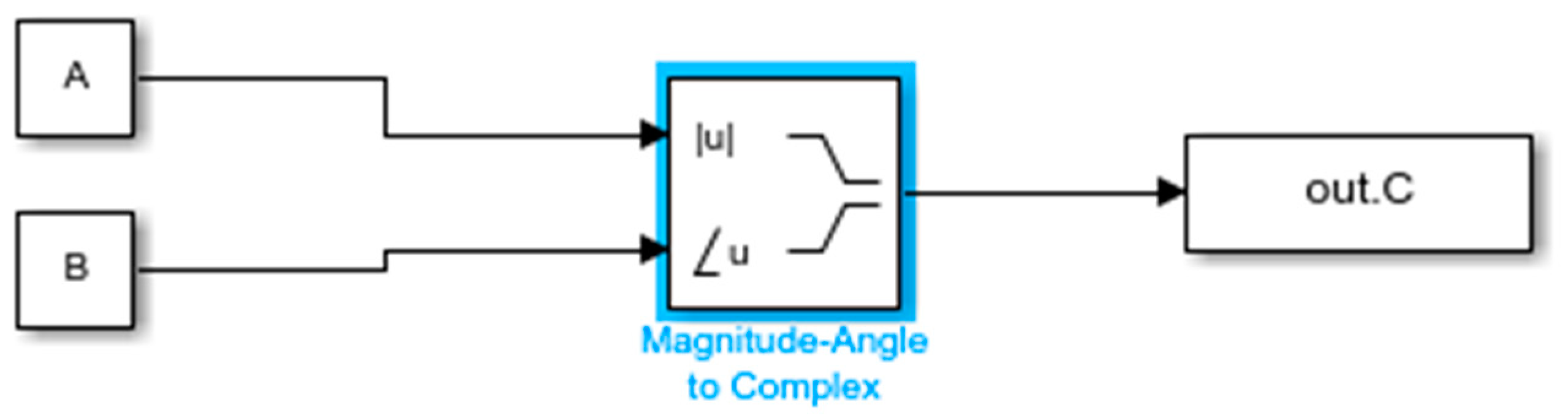
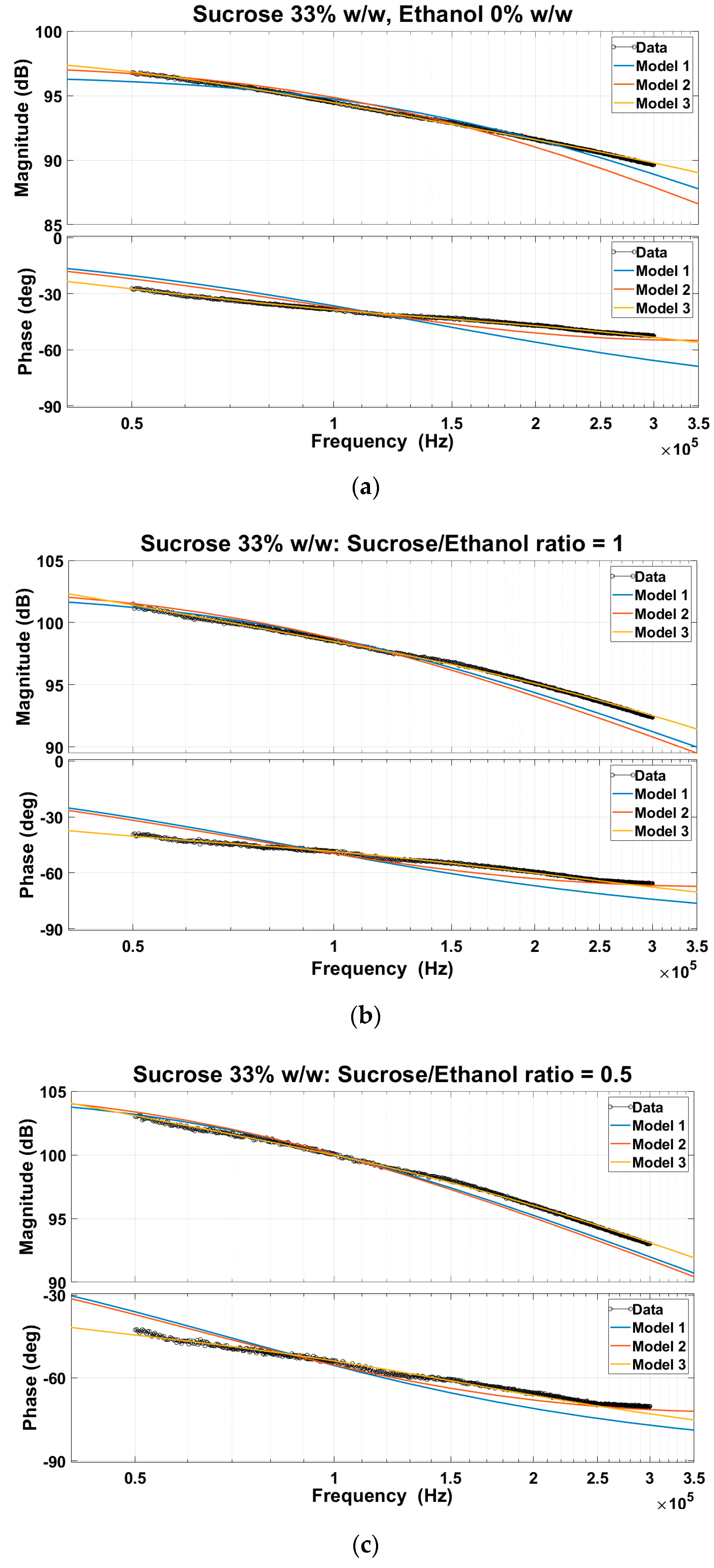
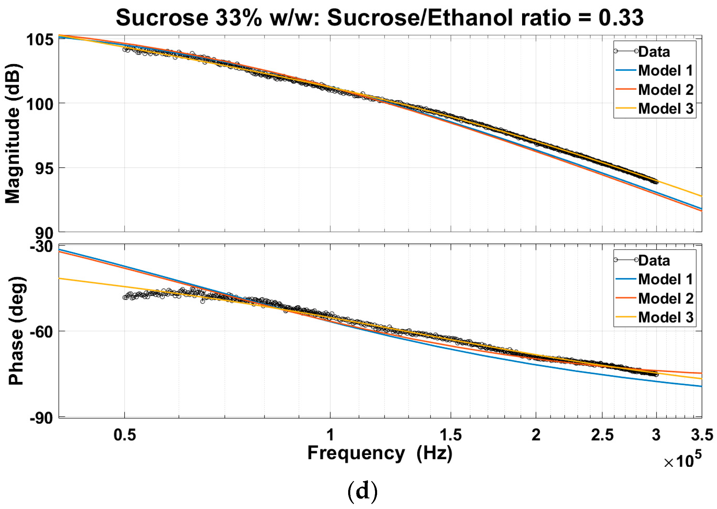
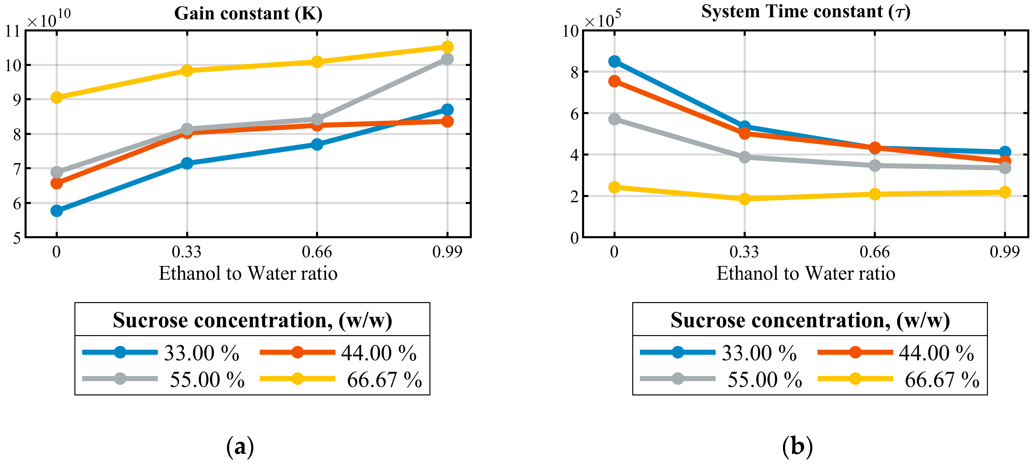
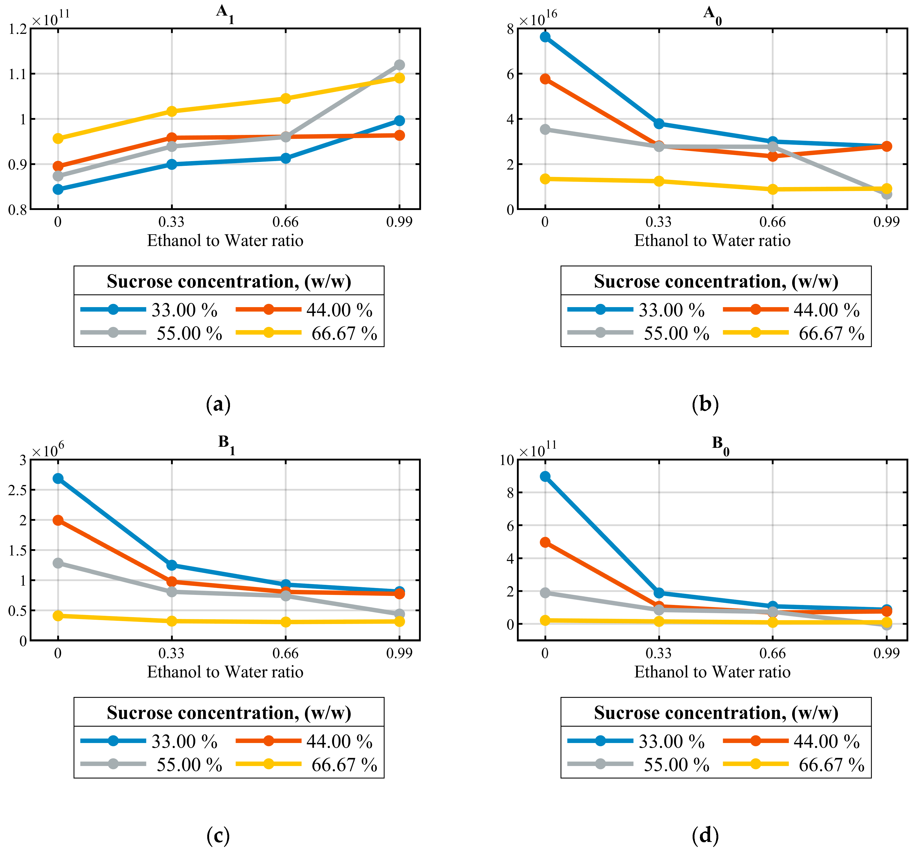
4.1.3. Creating Transfer Function Models from EIS Data and Comparative Analysis

The data points collected from the impedance spectroscope were imported into the MATLAB workspace for further processing. The phase angle was changed from degrees to radians using the function deg2rad. The impedance magnitude and phase in radians was converted into a rectangular complex number format. This complex variable was created using Magnitude–Angle to complex block using the Simulink® software. Figure 7 shows the Simulink program to autogenerate the complex variables for the recorded impedance spectra. This complex variable was further used to create a frequency response data (frd) model object in MATLAB.

In the Control System Toolbox™ of MATLAB, the frd models can be used to store, manipulate, and analyse frequency response data. The frd model stores a vector of frequency points with the corresponding complex frequency response data obtained either through simulations or experimentally. The MATLAB function used to create the frequency response data model object was: sysfrd = frd(sys,frequency,units).

Transfer function models describe the relationship between the inputs and outputs of a linear system using a ratio of polynomials. The model order is equal to the order of the denominator polynomial. The roots of the denominator polynomial are referred to as the model poles. The roots of the numerator polynomial are referred to as the model zeros. It describes the dynamic characteristics of the linear system. The transfer function of any linear invariant system G(s) can be expressed in general terms in the ratios of polynomials in terms of s as

$$G\left(s\right)=\frac{Y\left(s\right)}{X\left(s\right)}=\frac{b_m{s}^m+b_{m-1}{s}^{m-1}+\dots +b_0}{a_n{s}^n+a_{n-1}{s}^{n-1}+\dots +a_0} , m\le n$$

(12)

where X(s) is a system input signal in the Laplace domain, and Y(s) is the system output evoked by X(s). a₀ to a_n gives the coefficients of the numerator polynomial and b₀ to b_m gives the coefficients of the denominator polynomial. m is the number of zeroes, and n is the number of poles in the system. The equivalent factorized form of the transfer function is given as

$$\frac{Y\left(s\right)}{X\left(s\right)}=\frac{\left(s+z_1\right)\left(s+z_2\right)\dots \left(s+z_m\right)}{\left(s+p_1\right)\left(s+p_2\right)\dots \left(s+p_n\right)}$$

(13)

Here the z₁, z₂ …, z_m are zeroes of the system and p_1, p₂…, p_n are poles of the system.

The transfer function (tf) model object in the MATLAB Control System Toolbox represents the transfer function in a polynomial form. The data used for estimation was in the frequency range of 50 kHz and 300 kHz. First and second-order transfer functions were estimated for the experimental data from the generated system frd model object using the MATLAB function tfest: sys = tfest(data,np,nz). This function estimates a continuous-time transfer function, sys, using frequency–domain data (data) and contains (np) number of poles and (nz) number of zeroes.

Table 2. Transfer function models tested.

Model	Number of Poles	Number of Zeroes	Order of the Model
Model 1	1	0	First-order
Model 2	2	0	Second-order
Model 3	2	1	Second-order with a zero

shows the three models tested. The number of poles (np) was set to 1 and 2 to obtain a first-order and a second-order transfer function, respectively. The number of zeros in the sys by default was max(np-1,0).

The standard transfer function of the first-order inertial system is given by Equation (14). τ is the system time constant, and K is steady-state gain. This was the first model (Model 1) tested.

$$\frac{Y\left(s\right)}{X\left(s\right)}=\frac{K}{\tau s+1}$$

(14)

The second model (Model 2) tested was a second-order system as given by Equation (15). It has no zeroes and two poles.

$$\frac{Y\left(s\right)}{X\left(s\right)}=\frac{A_0}{B_2{s}^2+B_{1}s+B_0}$$

(15)

The third model (Model 3) tested was with two poles and one zero in the form of Equation (16).

$$\frac{Y\left(s\right)}{X\left(s\right)}=\frac{A_{1}s+A_0}{B_2{s}^2+B_{1}s+B_0}$$

(16)

Table 3. Sucrose to ethanol ratio at various concentration of sucrose solutions.

Solution Index	Effective Ethanol to Water Ratio	Different Concentrations of Sucrose Solutions (% w/w)	Effective Sucrose/Ethanol Ratio in 100 mL Solution	Tfest Fit %
				Model 1	Model 2	Model 3
1	0	33	-	55.2	67.8	96.43
2		44	-	55.56	68.48	95.84
3		55	-	62.31	76.26	93.42
4		66.67	-	88.98	80.12	91.75
5	0.33	33	1	64.87	63.73	95.12
6		44	1.33	71.26	72.85	94.95
7		55	1.66	78.31	76.86	92.33
8		66.67	2	89.94	80.51	90.9
9	0.66	33	0.5	74.3	65.82	94.74
10		44	0.66	75.82	79.5	94.88
11		55	0.83	80.38	81.39	92.03
12		66.67	1	91.5	83.07	92.92
13	0.99	33	0.33	79.22	89.45	93.29
14		44	0.44	79.1	90.27	94.13
15		55	0.55	83	91.61	92.07
16		66.67	0.66	92.11	92.2	93.74

shows the percentage fit to the data estimation (tfest fit %) of the transfer function fitted using Model 1, Model 2, and Model 3 for different working conditions, i.e. for different concentrations of sucrose solutions, and different effective ethanol to water ratios. The fit per cent is a quantitative assessment of the estimation of normalized root mean squared Error (NRMSE) measure of how well the response of the model fits the estimation data, expressed as the percentage fit = 100(1 – NRMSE). The fit percentage for Model 1 and Model 2 was higher at 55% w/w and 66.67% w/w solutions compared to the solutions with lower concentrations of 33% w/w and 44% w/w. However, the goodness of fit does not increase monotonically from Model 1 to Model 2. This issue was resolved in Model 3 by adding one zero to the second-order transfer function, which results in a good agreement between the experimental data and the response of the model with a minimum of 90.9 % fit for all the solutions.

Figure 8a–d shows the bode plot comparison of the fit of Model 1, Model 2, and Model 3 transfer functions to the acquired experimental data for the solution with sucrose concentration 33 % w/w at various ethanol to water ratios. The highest fit percentage of the Model 3 can be observed graphically using bode representation.

Figure 9a,b shows the change in model parameters: steady-state gain (K) and time constant ($\tau$), for various sucrose concentrations at increasing ethanol to water ratios evaluated using the first-order transfer function. It confirms that the considered system is nonlinear. However, for a constant working condition, a simplified linear model in the form of the transfer function can be applied. An increase in the gain constant K and a decrease in system time constant $\tau$ was observed as the ethanol to water ratio increased (Table 3), Model 1 could be used as a simple prediction tool with a limited accuracy.

Figure 10a–d shows the trend for the four coefficients A₁, A₀, B₁, and B₀ of the Model 3, and B₂ = 1. The increase in A₁ was observed as the ethanol to water ratio is increased, whereas a decrease was observed in the coefficients A₀, B₀, and B₁. The decrease in coefficients was greater for the lower concentration of ternary solutions of 33% w/w and 44% w/w as compared to the solutions with higher concentrations. The analysis of the model parameters shows a clear dependence between the concentration of the sucrose constituent component with EIS measurements. Accordingly, at a given sucrose concentration, the model parameters can be utilised to correspond to specific ethanol to water ratio present in the crystallizer. The variable domain obtained through the estimated transfer function model provides a framework to evaluate the concentration variation at a given operating condition during the antisolvent crystallization. This is an essential task that could lead to the design of a process control unit.

According to the current experimentation, the ternary chemical solution system can be modelled into a set of transfer functions containing poles and zeros based on the electrical impedances obtained within the frequency range. However, the present approach requires further investigation in order to increase the interpretability by limiting the variable space and obtain a fully usable system model. Such a system can be obtained using various methods such as principal component analysis [59] or development of a plausible equivalent electrical circuit via electrochemical modelling [31,60].

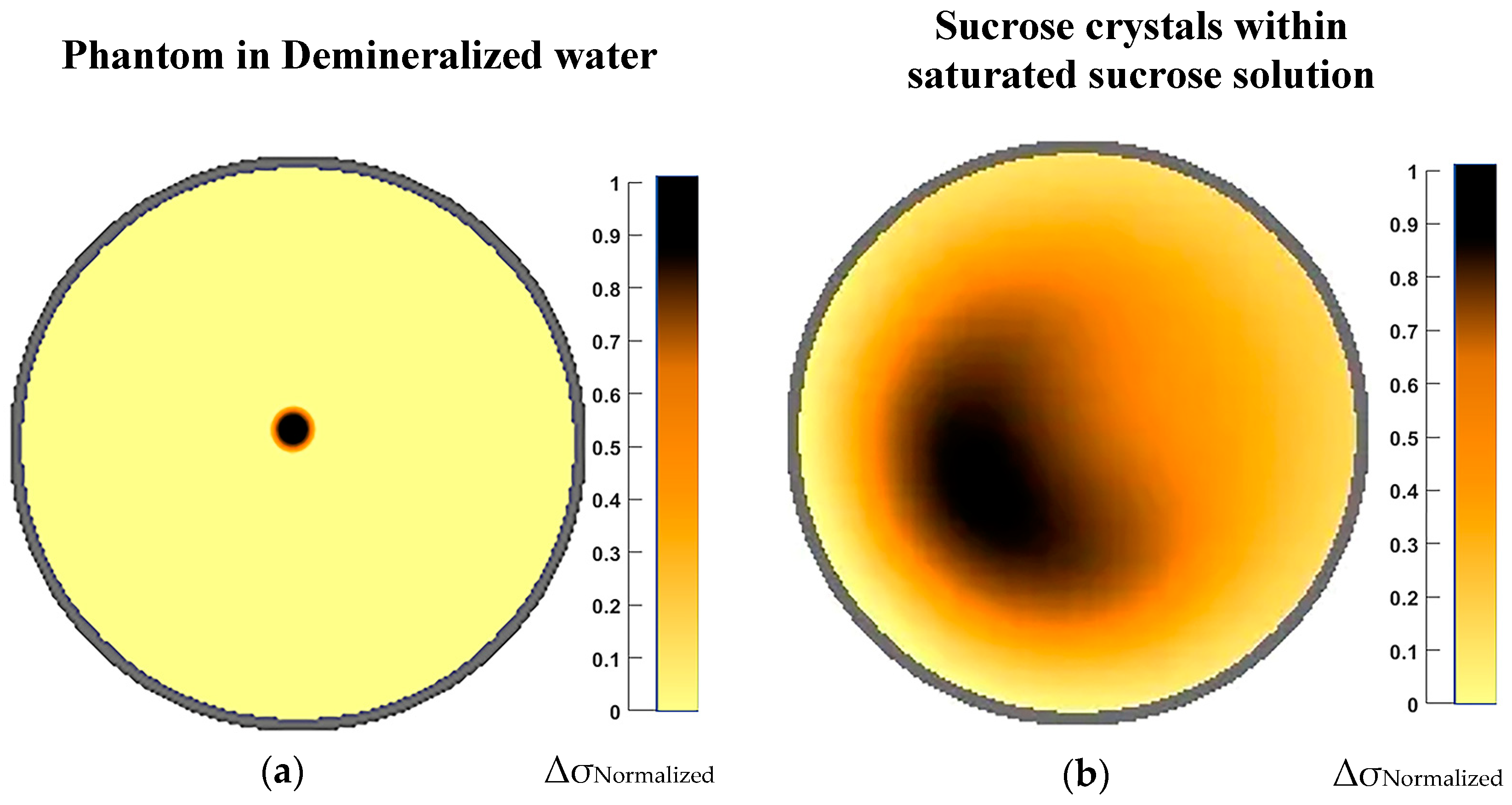
4.2. Results for Electrical Resistance Tomography Experiments

Figure 11a shows the voltage injections from the 16 electrodes (V1-V16) in the demineralized water, tap water, and industrial food grade saturated sucrose solution. The system was auto-calibrated for each solution. The voltage in millivolts injected was auto-determined by Roc-GUI software according to the conductivity of the solution under consideration. Figure 11b shows the current detected by each of the sensors in a single frame of record. The sensors closer to the source had higher currents, whereas the sensor away from the source had lower currents detected. The difference in the currents detected by the adjacent sink electrodes was higher than the sink electrodes located at the opposite periphery. A U-shaped pattern was visible due to the distance of the electrodes. The maximum absolute difference in currents measured using Equation (17) for tap water was 1.747 mA and the industrial food grade saturated sucrose solution was around 1.808 mA whereas for demineralized water, it was 0.191 mA.

$$\mathrm{Absolute} \mathrm{difference}=[\overline{\max ({\mathrm{F}}_{\mathrm{i}}\in \mathrm{v})}-\overline{\min ({\mathrm{F}}_{\mathrm{i}}\in \mathrm{v})}];$$

(17)

where F_i is the dataset of all currents (i1-i15) for sensor excited with voltage V.

Figure 12a displays the 10 mm ABS phantom reconstructed using the Bayesian method in sucrose solution. Figure 12b shows the qualitatively detected density distribution of the white sucrose crystals in the calibrated solution of industrial food grade saturated sucrose. Cross-sectional tomographic images acquired from the real-time measurements of the solid particle dispersion visualize non-conducting regions in the black colour. Since there is no mixing in the reactor, the particles are not uniformly distributed, and the agglomeration can be observed towards the left region. The images are mapped after normalizing the changes in the conductivity Δσ_Normalized from 0 to 1. Similar results were obtained using ERT techniques in gas hold up applications within stirred vessel [61].

5. Conclusions

In this research work, the feasibility of monitoring the antisolvent crystallization of sucrose using electrical impedance spectroscopy (EIS) was studied at laboratory scale. Herein, the impedance spectra of the ternary solutions of sucrose–water–ethanol acquired by 1-D thin electrodes were used to create a frequency response model. The parametric model was further developed to estimate a series of transfer functions of the measured impedances. According to the results, the experimental dataset of the ternary solutions in the frequency range of 50–300 kHz was in good agreement with a transfer function model containing two poles and a single zero (Model 3). This was established using a quantitative analysis performed by estimating the normalized root mean squared Error (NRMSE) measure to evaluate how well the response of the model fits the experimental data. The proposed approach has possibilities to detect the impedance variation according to concentration ratio during the crystallization process. The analysis of the model constants indicates a dependence between the concentration of the constituent component and the poles and zeros of the model (EIS measurements). In future studies, more complex component analysis can be carried out to limit the variable space and identify the behaviour of the impedances for a given operating condition during the antisolvent crystallization.

Furthermore, a 2-D electrical resistance tomography (ERT) system with a low conductivity sensor unit was designed and tested with demineralized water, tap water and industrial food grade saturated sucrose solution. Low conductivity region of sucrose particles concentration was observed and reconstructed in real-time using Bayesian reconstruction methodology. This study provides the possibility of utilizing the EIS and ERT as complementary PAT methods to control sucrose manufacturing. Upon future investigations, additional development of these process monitoring modalities with different conductivity profiles could provide a multi-frequency ERT sensor that can be applied for antisolvent crystallization process monitoring and quality assurance. A multi-sensor based semi-empirical approach for monitoring status, application of control, and visualization of the distribution of crystalline solids are foreseen.

References

1. Simon, L.L.; Simone, E.; Oucherif, K.A. Crystallization process monitoring and control using process analytical technology. In Software Architectures and Tools for Computer Aided Process Engineering; Elsevier BV: Amsterdam, The Netherlands, 2018; Volume 41, pp. 215–242. [Google Scholar]
2. Claßen, J.; Aupert, F.; Reardon, K.F.; Solle, D.; Scheper, T. Spectroscopic sensors for in-line bioprocess monitoring in research and pharmaceutical industrial application. Anal. Bioanal. Chem. 2016, 409, 651–666. [Google Scholar] [CrossRef]
3. Simone, E.; Saleemi, A.N.; Nagy, Z.K. In Situ Monitoring of Polymorphic Transformations Using a Composite Sensor Array of Raman, NIR, and ATR-UV/vis Spectroscopy, FBRM, and PVM for an Intelligent Decision Support System. Org. Process. Res. Dev. 2014, 19, 167–177. [Google Scholar] [CrossRef]
4. Sankowski, D.; Sikora, J. Electrical Capacitance Tomography: Theoretical Basis and Applications; Wydawnictwo Książkowe Instytutu Elektrotechniki: Warszawa, Poland, 2010. [Google Scholar]
5. Grudzien, K.; Chaniecki, Z.; Romanowski, A.; Niedostatkiewicz, M.; Sankowski, D. ECT Image Analysis Methods for Shear Zone Measurements during Silo Discharging Process. Chin. J. Chem. Eng. 2012, 20, 337–345. [Google Scholar] [CrossRef]
6. Ricard, F.; Brechtelsbauer, C.; Xu, Y.; Lawrence, C.; Thompson, D. Development of an Electrical Resistance Tomography Reactor for Pharmaceutical Processes. Can. J. Chem. Eng. 2008, 83, 11–18. [Google Scholar] [CrossRef]
7. Koulountzios, P.; Rymarczyk, T.; Soleimani, M. A Quantitative Ultrasonic Travel-Time Tomography to Investigate Liquid Elaborations in Industrial Processes. Sensors 2019, 19, 5117. [Google Scholar] [CrossRef] [Green Version]
8. Rymarczyk, T.; Polakowski, K.; Sikora, J. A new concept of discretisation model for imaging improving in ultrasound transmission tomography. Inform. Autom. Pomiary Gospod. Ochr. Środowiska 2019, 49, 48–51. [Google Scholar]
9. Majchrowicz, M.; Kapusta, P.; Jackowska-Strumiłło, L.; Banasiak, R.; Sankowski, D. Multi-GPU, Multi-Node Algorithms for Acceleration of Image Reconstruction in 3D Electrical Capacitance Tomography in Heterogeneous Distributed System. Sensors 2020, 20, 391. [Google Scholar] [CrossRef] [Green Version]
10. Garbaa, H.; Jackowska-Strumiłło, L.; Grudzien, K.; Romanowski, A. Application of electrical capacitance tomography and artificial neural networks to rapid estimation of cylindrical shape parameters of industrial flow structure. Arch. Electr. Eng. 2016, 65, 657–669. [Google Scholar] [CrossRef]
11. Rymarczyk, T.; Kłosowski, G.; Kozłowski, E.; Tchórzewski, P. Comparison of Selected Machine Learning Algorithms for Industrial Electrical Tomography. Sensors 2019, 19, 1521. [Google Scholar] [CrossRef] [Green Version]
12. Nagy, Z.K.; Fujiwara, M.; Braatz, R.D.; Myerson, A.S.; Erdemir, D.; Lee, A.Y. Monitoring and Advanced Control of Crystallization Processes. Handb. Ind. Cryst. 2019, 313–345. [Google Scholar] [CrossRef]
13. Lewis, A.; Seckler, M.M.; Kramer, H.; Van Rosmalen, G. Industrial Crystallization; Cambridge University Press (CUP): Cambridge, UK, 2015. [Google Scholar]
14. Nagy, Z.K.; Braatz, R.D. Advances and New Directions in Crystallization Control. Annu. Rev. Chem. Biomol. Eng. 2012, 3, 55–75. [Google Scholar] [CrossRef] [PubMed] [Green Version]
15. Yu, Z.-Q.; Chow, P.S.; Tan, R.B.H. Application of Attenuated Total Reflectance−Fourier Transform Infrared (ATR−FTIR) Technique in the Monitoring and Control of Anti-solvent Crystallization. Ind. Eng. Chem. Res. 2006, 45, 438–444. [Google Scholar] [CrossRef]
16. Nowee, S.M.; Abbas, A.; Romagnoli, J.A. Antisolvent crystallization: Model identification, experimental validation and dynamic simulation. Chem. Eng. Sci. 2008, 63, 5457–5467. [Google Scholar] [CrossRef]
17. Bhangu, S.K.; AshokKumar, M.; Lee, J. Ultrasound Assisted Crystallization of Paracetamol: Crystal Size Distribution and Polymorph Control. Cryst. Growth Des. 2016, 16, 1934–1941. [Google Scholar] [CrossRef]
18. Lee, J.; AshokKumar, M.; Kentish, S. Influence of mixing and ultrasound frequency on antisolvent crystallisation of sodium chloride. Ultrason. Sonochemistry 2014, 21, 60–68. [Google Scholar] [CrossRef]
19. El Bazi, W.; Porte, C.; Mabille, I.; Havet, J.-L. Antisolvent crystallization: Effect of ethanol on batch crystallization of α glycine. J. Cryst. Growth 2017, 475, 232–238. [Google Scholar] [CrossRef]
20. Lindenberg, C.; Krattli, M.; Cornel, J.; Mazzotti, M.; Brozio, J. Design and Optimization of a Combined Cooling/Antisolvent Crystallization Process. Cryst. Growth Des. 2009, 9, 1124–1136. [Google Scholar] [CrossRef]
21. Howard, K.S.; Nagy, Z.K.; Saha, B.; Robertson, A.L.; Steele, G.; Martin, D. A Process Analytical Technology Based Investigation of the Polymorphic Transformations during the Antisolvent Crystallization of Sodium Benzoate from IPA/Water Mixture. Cryst. Growth Des. 2009, 9, 3964–3975. [Google Scholar] [CrossRef]
22. Boukamp, B.; Denisov, D.; Hassanizadeh, M.; Hessling, D.; Huinink, H.; Karadimitriou, N.; Kuijpers, K.; Ravensbergen, J.; Sabater, C.; Schoemaker, F. Analyzing liquid penetration in paper by electrical impedance spectroscopy (EIS). Proc. Phys. Ind. 2013, 4, 25–44. [Google Scholar]
23. Randviir, E.P.; Banks, C.E. Electrochemical impedance spectroscopy: An overview of bioanalytical applications. Anal. Methods 2013, 5, 1098. [Google Scholar] [CrossRef]
24. Jiang, Z.; Yao, J.; Wang, L.; Wu, H.; Huang, J.; Zhao, T.; Takei, M. Development of a Portable Electrochemical Impedance Spectroscopy System for Bio-Detection. IEEE Sens. J. 2019, 19, 5979–5987. [Google Scholar] [CrossRef]
25. Santoso, D.R.; Pitaloka, B.; Widodo, C.S.; Juswono, U.P. Low-Cost, Compact, and Rapid Bio-Impedance Spectrometer with Real-Time Bode and Nyquist Plots. Appl. Sci. 2020, 10, 878. [Google Scholar] [CrossRef] [Green Version]
26. Conesa, C.; Garcia-Breijo, E.; Loeff, E.; Segui, L.; Fito, P.J.; Miró, N.L. An Electrochemical Impedance Spectroscopy-Based Technique to Identify and Quantify Fermentable Sugars in Pineapple Waste Valorization for Bioethanol Production. Sensors 2015, 15, 22941–22955. [Google Scholar] [CrossRef] [PubMed] [Green Version]
27. Grossi, M.; Riccò, B. Electrical impedance spectroscopy (EIS) for biological analysis and food characterization: A review. J. Sens. Sens. Syst. 2017, 6, 303–325. [Google Scholar] [CrossRef] [Green Version]
28. Zhao, Y.; Wang, M.; Hammond, R.B. Characterization of crystallisation processes with electrical impedance spectroscopy. Nucl. Eng. Des. 2011, 241, 1938–1944. [Google Scholar] [CrossRef]
29. Zhao, Y.; Yao, J.; Wang, M. On-line monitoring of the crystallization process: Relationship between crystal size and electrical impedance spectra. Meas. Sci. Technol. 2016, 27, 074007. [Google Scholar] [CrossRef] [Green Version]
30. Chakraborty, S.; Das, C.; Bera, N.K.; Chattopadhyay, S.; Karmakar, A.; Chattopadhyay, S. Analytical modelling of electrical impedance based adulterant sensor for aqueous sucrose solutions. J. Electroanal. Chem. 2017, 784, 133–139. [Google Scholar] [CrossRef]
31. Eder, C.; Briesen, H. Impedance spectroscopy as a process analytical technology (PAT) tool for online monitoring of sucrose crystallization. Food Control. 2019, 101, 251–260. [Google Scholar] [CrossRef]
32. Villanueva, D.; Posada, R.; Gonzalez, I.; García, Á.; Martinez-Sibaja, A. Monitoring of a Sugar Crystallization Process with Fuzzy Logic and Digital Image Processing. J. Food Process Eng. 2014, 38, 19–30. [Google Scholar] [CrossRef]
33. Subbiah, B.; Morison, K.R. Electrical conductivity of viscous liquid foods. J. Food Eng. 2018, 237, 177–182. [Google Scholar] [CrossRef]
34. Rao, G.; Sattar, M.A.; Wajman, R.; Jackowska-Strumillo, L. Application of the 2D-ERT to evaluate phantom circumscribed regions in various sucrose solution concentrations. In Proceedings of the 2019 International Interdisciplinary PhD Workshop (IIPhDW), Wismar, Germany, 15–17 May 2019; pp. 34–38. [Google Scholar]
35. Yang, Z.J.; Yan, G. Detection of Impact Damage for Composite Structure by Electrical Impedance Tomography. In ACMSM25; Springer: Berlin/Heidelberg, Germany, 2019; pp. 519–527. [Google Scholar]
36. Clausi, M.; Toto, E.; Botti, S.; Laurenzi, S.; La Saponara, V.; Santonicola, M.G. Direct effects of UV irradiation on graphene-based nanocomposite films revealed by electrical resistance tomography. Compos. Sci. Technol. 2019, 183, 107823. [Google Scholar] [CrossRef]
37. Ghaednia, H.; Owens, C.; Roberts, R.; Tallman, T.N.; Hart, A.J.; Varadarajan, K.M. Interfacial load monitoring and failure detection in total joint replacements via piezoresistive bone cement and electrical impedance tomography. Smart Mater. Struct. 2020. [Google Scholar] [CrossRef] [Green Version]
38. Salazar, A.J.; Bravo, R.J.; Murrugara, C.; Osberth, O.C.; Farkas, E.; Gravis, K.; Gavidia, L. Proposal for a real-time multi-frequency impedance tomography system. In Proceedings of the 3rd European Medical and Biological Engineering Conference, Prague, Czech Republic, 20–25 November 2005; Volume 11, pp. 1727–1983. [Google Scholar]
39. Yang, Y.; Jia, J. A multi-frequency electrical impedance tomography system for real-time 2D and 3D imaging. Rev. Sci. Instrum. 2017, 88, 85110. [Google Scholar] [CrossRef]
40. Hampel, U.; Wondrak, T.; Bieberle, M.; Lecrivain, G.; Schubert, M.; Eckert, K.; Reinecke, S.F. Smart Tomographic Sensors for Advanced Industrial Process Control TOMOCON. Chem. Ing. Tech. 2018, 90, 1238–1239. [Google Scholar] [CrossRef] [Green Version]
41. Schiefelbein, S.L.; Fried, N.A.; Rhoads, K.G.; Sadoway, D.R. A high-accuracy, calibration-free technique for measuring the electrical conductivity of liquids. Rev. Sci. Instrum. 1998, 69, 3308–3313. [Google Scholar] [CrossRef]
42. Barsukov, E.; Macdonald Ross, J. Impedance Spectroscopy. In Theory, Experiment and Applications; Wiley-Interscience: New York, NY, USA, 2005. [Google Scholar]
43. Orazem, M.E.; Tribollet, B. Electrochemical Impedance Spectroscopy; John Wiley & Sons: Hoboken, NJ, USA, 2017. [Google Scholar]
44. Nahvi, M.; Hoyle, B.S. Electrical Impedance Spectroscopy Sensing for Industrial Processes. IEEE Sens. J. 2009, 9, 1808–1816. [Google Scholar] [CrossRef]
45. Ramos, P.M. How signal processing is changing impedance spectroscopy. In Proceedings of the 2018 IEEE International Instrumentation and Measurement Technology Conference (I2MTC), Houston, TX, USA, 14–17 May 2017; IEEE: New York, NY, USA, 2018; pp. 1–6. [Google Scholar]
46. Wu, J.; Stark, J.P.W. A high accuracy technique to measure the electrical conductivity of liquids using small test samples. J. Appl. Phys. 2007, 101, 054520. [Google Scholar] [CrossRef]
47. Becchi, M.; Avendaño, C.; Strigazzi, A.; Barbero, G. Impedance Spectroscopy of Water Solutions: The Role of Ions at the Liquid−Electrode Interface. J. Phys. Chem. B 2005, 109, 23444–23449. [Google Scholar] [CrossRef]
48. Longo, J.P.N.; Galvão, J.R.; da Silva, J.C.C.; Martelli, C.; Morales, R.E.M.; da Silva, M.J. Dual sensor for simultaneous measurement of electrical impedance and temperature during ice formation process. In Proceedings of the 2nd International Symposium on Instrumentation Systems, Circuits and Transducers (INSCIT), Ceara, Brazil, 28 August–1 September 2017; IEEE: New York, NY, USA, 2017; pp. 1–4. [Google Scholar]
49. Juansah, J.; Yulianti, W. Studies on Electrical behavior of Glucose using Impedance Spectroscopy. In IOP Conference Series: Earth and Environmental Science; IOP Publishing: Bristol, UK, 2016; Volume 31, p. 012039. [Google Scholar]
50. Rane, M.V.; Uphade, D.B. Energy Efficient Jaggery Making Using Freeze Pre-concentration of Sugarcane Juice. Energy Procedia 2016, 90, 370–381. [Google Scholar] [CrossRef]
51. Liu, Q.; Han, Y.; Zhang, X. An image reconstruction algorithm based on Bayesian theorem for electrical resistance tomography. Optik 2014, 125, 6090–6097. [Google Scholar] [CrossRef]
52. Rymarczyk, T.; Tchórzewski, P.; Sikora, J. Coupling boundary element method with level set method to solve inverse problem. Inform. Autom. Pomiary Gospod. Ochr. Środowiska 2017, 7, 80–83. [Google Scholar] [CrossRef]
53. Kim, B.S.; Khambampati, A.K.; Jang, Y.J.; Kim, K.-Y.; Kim, S. Image reconstruction using voltage–current system in electrical impedance tomography. Nucl. Eng. Des. 2014, 278, 134–140. [Google Scholar] [CrossRef]
54. Vaukonen, M. Electrical Impedance Tomography and Prior Information. Ph.D. Thesis, University of Kuopio, Kuopio, Finland, 1997. [Google Scholar]
55. Cui, Z.; Wang, Q.; Xue, Q.; Fan, W.; Zhang, L.; Cao, Z.; Sun, B.; Wang, H.; Yang, W. A review on image reconstruction algorithms for electrical capacitance/resistance tomography. Sens. Rev. 2016, 36, 429–445. [Google Scholar] [CrossRef]
56. Lionheart, W.R.B. EIT reconstruction algorithms: Pitfalls, challenges and recent developments. Physiol. Meas. 2004, 25, 125–142. [Google Scholar] [CrossRef] [Green Version]
57. Adler, A.; Lionheart, W.R.B. Uses and abuses of EIDORS: An extensible software base for EIT. Physiol. Meas. 2006, 27, S25–S42. [Google Scholar] [CrossRef] [Green Version]
58. Persson, P.-O.; Strang, G. A Simple Mesh Generator in MATLAB. SIAM Rev. 2004, 46, 329–345. [Google Scholar] [CrossRef] [Green Version]
59. Marć, M.; Bystrzanowska, M.; Tobiszewski, M. Exploratory analysis and ranking of analytical procedures for short-chain chlorinated paraffins determination in environmental solid samples. Sci. Total. Environ. 2020, 711, 134665. [Google Scholar] [CrossRef]
60. Olarte, O.; Barbé, K.; Van Moer, W.; Van Ingelgem, Y.; Hubin, A. Measurement and characterization of glucose in NaCl aqueous solutions by electrochemical impedance spectroscopy. Biomed. Signal Process. Control. 2014, 14, 9–18. [Google Scholar] [CrossRef]
61. Sardeshpande, M.V.; Gupta, S.; Ranade, V.V. Electrical resistance tomography for gas holdup in a gas-liquid stirred tank reactor. Chem. Eng. Sci. 2017, 170, 476–490. [Google Scholar] [CrossRef] [Green Version]
Figure 1. (a) Schematic showing antisolvent crystallization; (b) sucrose–water phase equilibrium diagram, Reproduced with permission from [50], Elsevier, 2016.
Applsci 10 03903 g001
Figure 2. (a) Voltage injected-current detected based electrical resistance tomography (ERT) system schematic; (b) finite element method (FEM) mesh created using EIDORS.
Applsci 10 03903 g002
Figure 3. (a) Experimental setup for the impedance spectroscopy testing unit with reactor placed over magnetic stirrer and syringe pump; (b) impedance spectrometer.
Applsci 10 03903 g003
Figure 4. (a) Sensor mounted with the low conductivity signal processing unit; (b) ERT data acquisition flow and reconstruction system.
Applsci 10 03903 g004
Figure 5. Impedance magnitude and phase response for sucrose solution before ethanol addition from 1 kHz to 1 MHz (a,b) from 50 kHz to 300 kHz (c,d).
Applsci 10 03903 g005
Figure 6. Impedance magnitude and phase response of the solutions at ethanol to water ratio; 0.33 (a,b), 0.66 (c,d), and 0.99 (e,f) for the frequency range from 50 kHz to 300 kHz. Table 1 lists all the solutions.
Applsci 10 03903 g006
Figure 7. Simulink program used to convert from rectangular coordinates to complex coordinates. The output data was used to create an frd model object.
Applsci 10 03903 g007
Figure 8. Bode plot comparisons of acquired data with transfer function models for sucrose 33% w/w and (a) 0% ethanol, (b) sucrose to Ethanol ratio 1, (c) sucrose to Ethanol ratio 0.5, (d) sucrose to ethanol ratio 0.33. Table 3 shows effective sucrose to ethanol ratios for all the solutions.
Applsci 10 03903 g008aApplsci 10 03903 g008b
Figure 9. Changes of Model 1 parameters. (a) Gain constant K; (b) system time constant τ , for different working conditions.
Applsci 10 03903 g009
Figure 10. Parameters of Model 3 for various working conditions, where: coefficients in numerator (a) A1, (b) A0 and denominator (c) B1, (d) B0, and B2 = 1.
Applsci 10 03903 g010
Figure 11. (a) Voltage injections at the sensor for a frame, (b) Current detections through the sensors.
Applsci 10 03903 g011
Figure 12. Tomographic reconstructions indicating conductivity changes ΔσNormalized (a) A 10 mm phantom inside demineralized water (b) density distribution of the sucrose crystals within industrial food grade saturated sucrose solution.
Applsci 10 03903 g012