Abstract
Minimizing energy consumption is significant for the hydraulic walking robot to reduce its power unit weight and increase working hours. However, most robot leg designs are inefficient due to their bio-mimetic or mission-specific mechanical structure. This paper presents a structural optimization method of the hydraulic walking robot by optimizing its mechanical structure and gait parameters simultaneously. The mathematical model of the total power of the hydraulic hexapod robot (HHR) is established, which is derived based on a general template for designing the hydraulic walking robot. The archive-based micro genetic algorithm (AMGA) is used to optimize the highly nonlinear multi-constraint multi-objective optimizations. In the optimal solution, the energy consumption of the HHR has reduced more than 40% by comparison with the original mechanical structure and gait parameter. Design sensitivity analysis is carried out to determine the regulation of mechanical structure, and a virtual prototype is used to verify the effectiveness of the proposed methods.
1. Introduction
Over the last decades, bionic legged robots have been developed to increase transportation adaption in mountainous areas, fieldwork, military activities, and other non-structural environments [1]. In hydraulics, advanced walking robots have been developed in succession, for example, Boston Dynamics’ Bigdog [2] and Atlas [3], IIT’s HyQ [4] and HyQ2Max [5], Shandong University’s SCalf-III [6], Delft University’s TU Delft [7], NTUA’s HexaTerra [8], and Ritsumeikan University’s TaeMu [9]. In addition to these advanced high-tech robots, the actuation of hydraulics has the significant advantage of high power-to-mass ratio, fast dynamic response, and large force output with no gears required compared with electric actuators [10]. However, the hydraulic walking robot is also less efficient [11], which limits its load-carrying capacity and working hours for field applications. Therefore, it is of great significance to reduce the energy consumption of hydraulic walking robots.
A variety of approaches have been proposed to reduce the energy consumption in terms of hydraulic driving system, mechanical structure, and motion planning algorithm. From the perspective of the hydraulic system, valve control systems [12] are mostly used in the hydraulic walking robot with the advantage of fast response and high precision control. Koivumäki et al. [13] proposed a separate meter-in separate meter-out (SMISMO) hydraulic control system, and the actuators’ energy consumption was reduced by 45% without noticeable motion control deterioration. Xue et al. [14] proposed a novel hydraulic system based on the two-stage pressure source, and the energy efficiency was increased by 41.5% compared to the single-stage hydraulic system. Du et al. [15] proposed a load-prediction based method to reduce valve throttling energy loss, in which the supply pressure was varied to track the force required by any actuator branch. Experimental results showed that hydraulic power savings of up to 70% were achieved. Most of the improvements in hydraulic driving system are too complicated to apply, and more studies are focused on structural design and gait optimization. Zhao et al. [16] presented a structural optimization method to change the arrangement of the planar redundant actuator, and the energy consumption of the parallel hydraulic mechanism was reduced by 10%. Rezazadeh et al. [17] presented a general theorem for designing a mechanism based on a template with biological relevance for a wide range of tasks. The design of the mechanical structure improved the walking energy efficiency by more than 50%. Ma et al. [18] reduced the hydraulic flow of the quadruped robot, and particle swarm optimization algorithm (PSO) was used to optimize the mechanical design parameters of the robot. Some scholars optimized the mechanism design from the aspect of hydraulic actuators [19,20], and the elastic load suspension mechanism was also used to improve energy efficiency [21,22]. In the study of energy consumption of hydraulic walking robots, the intelligent motion planning algorithm is determined to reduce energy consumption [23]. Yang et al. [24,25] established an energy model including the mechanical power and heat rate and optimized the quadruped robot foot trajectory from the aspects of step height, step length, standing height, gait cycle, and duty cycle. The total joint energy consumption in simulations and experiments dropped by 8.02% and 7.55%, respectively. Gao et al. [26] presented a method to minimize the energy consumption by 19.35% by providing an integrated strategy of motion planning subject to velocity and acceleration constraints. However, few of these studies reduce the total energy consumption of the hydraulic driving system of the legged robot, and the mechanical structure and motion trajectory are rarely optimized at the same time.
The optimization of the hydraulic legged robot has multiple parameters, objective functions, and restrictions. Therefore, the traditional optimization method may face the problem of extensive computation, slow convergence, and non-optimal solutions. Several optimization algorithms have been applied to facilitate the multi-objective constrained problem. Park et al. [27] conducted the kinematic parameter optimization of 2DOF (two degrees of freedom) redundantly actuated parallel mechanism via the Taguchi method. The quasi-optimized results were derived after the second stage of optimization, which promises robust optimization results even if the user’s working conditions change. Zhu et al. [28] applied the genetic algorithm (GA) with inverse kinematics and trajectory planning in a gait period to solve the optimization problem. The optimal parameters not only satisfied the requirement of the target workspace but also achieved the minimum energy consumption and lower joint torques. Ren et al. [29] used the archive-based micro genetic algorithm (AMGA) to optimize the leg structure of the linkage quadruped robot, which was particularly suitable for solving highly nonlinear multi-constraint multi-objective optimizations. Ha et al. [30] obtained the complicated relationship between design and motion parameters via sensitivity analysis, and the joint torque was reduced by 40% based on the implicit function theorem. Edgar et al. [31] proposed a non-parametric convex optimization program for the design of the nonlinear elastic element that minimized energy consumption and peak power for an arbitrary periodic reference trajectory. Satoru et al. [32] proposed a fast computation method based on the Casimir function and Hamiltonian function, and almost 50% of the computational cost for the optimization of high degree of freedom hydraulic arms and legs were cut. At present, the optimization methods for the legged robot are few, and more intelligent algorithms can be developed.
This work focuses on the mechanical design and gait optimization of a hydraulic hexapod robot to reduce energy consumption. It provides a structure procedure to maximize the energy efficiency and maintains bio-inspired factors for the control and versatility for a hydraulic walking robot. First, the mathematical model of the total power of the hydraulic hexapod robot (HHR) with a novel leg structure is established. The pressure and flow rate of the hydraulic driving system of the robot is derived based on a general template for designing the hydraulic walking robot. Then, the archive-based micro genetic algorithm (AMGA) is used to optimize the objective function with multiple structural variables. The energy consumption of the optimized result is compared with the original mechanical structure and gait parameter. Finally, design sensitivity analysis is carried out and a virtual prototype is used to verify the effectiveness of the proposed methods.
2. Modeling and Design Process
As shown in Figure 1, the HHR is designed according to the mammalian structure with a body and six legs. Hexapod robots can walk with different gaits to overcome various terrains and have a higher load-bearing capacity and stability than bipedal and quadrupedal robots [33]. The legs of HHRs adopt the same mechanism, which are designed as a 3DOF (degree of freedom) structure to meet the hexapod gaits requirements. The area of the middle leg cylinders is twice as much as the others. The driving hydraulic cylinders for the hip joint and knee joint are fixed on the thigh, and the root joint cylinder is set on the pelvis, as shown in Figure 1.
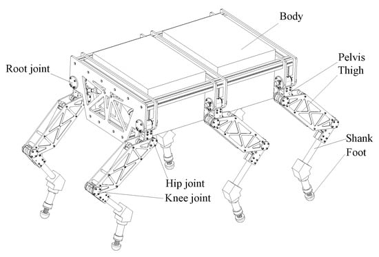
Figure 1.
Hydraulic hexapod robot.
In this paper, an integrated modeling-optimizing robot design process is proposed where the modeling steps are combined with the optimal structural design process, as shown in Figure 2. The optimization stage formulates the problem based on the modeling stage, and the robot structure is regulated according to the optimal solution.
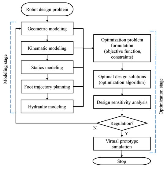
Figure 2.
Robot modeling and design process.
The modeling stage starts with geometric modeling, which illustrates the leg structure of the HHR and the relationship between the cylinder and joint angle. The kinematic model is established to find the relation between the foot position and joint angles based on the Denavit–Hartenberg (D-H) homogenous matrix representation. Inverse kinematics and Jacobian matrix of the single leg is derived. By statics modeling, the joint output force and walking stability margin are obtained. Foot trajectory planning is analyzed based on the HHR motion requirement, and the length and velocity of the cylinders are achieved with the geometric and kinematic model. Combined with the above results, the model of the hydraulic driving system is established to calculate the flow rate and pressure for each cylinder as well as the overall energy consumption for the HHR.
The optimization stage is a process that consists of optimization problem formulation, optimal design solutions, and design sensitivity analysis. In the optimization problem formulation step, flow rate, maximum pressure, and stability margin are defined as objective functions with appropriate constraints. In order to improve computing efficiency, the archive-based micro genetic algorithm (AMGA) is applied to find the optimal design solutions in the next step. Design sensitivity analysis is used to determine the changes needed to regulate the mechanical structure and gait parameter for installation and manufacture requirements. The virtual prototype is employed to prove the optimization result is reasonable and reliable.
Before modeling the robot, the following preconditions are made:
- (a)
- The robot is walking on a flat surface with triangle gait, and the height change of the robot body’s center of mass (COM) is ignored.
- (b)
- The payload of the HHR is far more than the leg mass, so gravity and inertial force of the leg components are ignored.
- (c)
- When the HHR moves at a constant speed, the ground friction force can be ignored, and the contact force on the foot can be supposed as vertical upward.
- (d)
- The pressure of the cylinder chamber is lower than the system pressure and greater than zero.
3. Robot Modeling
3.1. Geometric Modeling
Reasonable leg structure design is vital to the mobility of a legged robot. As shown in Figure 3, a novel leg structure is adopted in the HHR. The hip and knee cylinders are fixed on the thigh, and the installation points of the cylinder are on both sides of the joint connection line. In the structure, the space for installation is reduced and the arm of force for cylinders can be increased. L1, L2 are the length of the thigh and shank. θ0, θ1, θ2 are the angles of the root, hip, and root joint. a0, a1, a2, b0, b1, b2, e01, e02, e11, e12, e21, e22 are variables for the cylinders’ installation. c0, c1, c2 and l0, l1, l2 are the cylinders’ length and arm of force for root, hip, and knee joint.
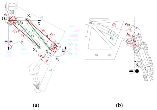
Figure 3.
Geometric parameters of the leg structure: (a) hip and knee joint; (b) root joint.
According to Figure 3a, the length of the hydraulic cylinder and the arm of the force can be obtained according to the geometrical relationship, where
Combining Equations (1) and (2), the velocity of the cylinders of leg i (i = 1–6) can be obtained as
3.2. Kinematic Modeling
The initial posture and the general posture are shown in Figure 4 and the D-H parameters are shown in Table 1.
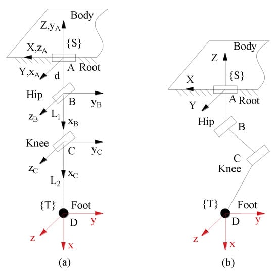
Figure 4.
Leg posture and coordinate frames: (a) initial posture; (b) general posture.

Table 1.
Denavit–Hartenberg (D-H) parameters for the 3DOF (3 degrees of freedom) leg.
The transformation matrix from the foot coordinate system to the body one at a general configuration can be written as
According to Equation (6), the joint angles can be obtained through inverse displacement analysis, and two solutions are obtained. Given the range of joint angles, the following solution is chosen.
where
The Jacobian matrix of the single leg model can also be calculated by Equation (6).
where
3.3. Statics Modeling
The HHR structural diagram is illustrated in Figure 5. The HHR moves with triangle gait, and the supporting points on the ground are shown in Figure 6. The vertical projection of the center of mass (COM) should be inside the supporting triangle to ensure the motion stability. The distance from the projection point to the three sides of the supporting triangle is the stability margin of the robot motion. Considering that the robot may be subjected to lateral impact, the stability margin should be as large as possible.
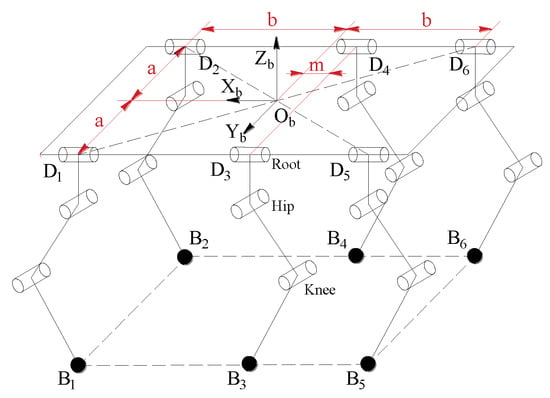
Figure 5.
Structure diagram of the hydraulic hexapod robot (HHR).
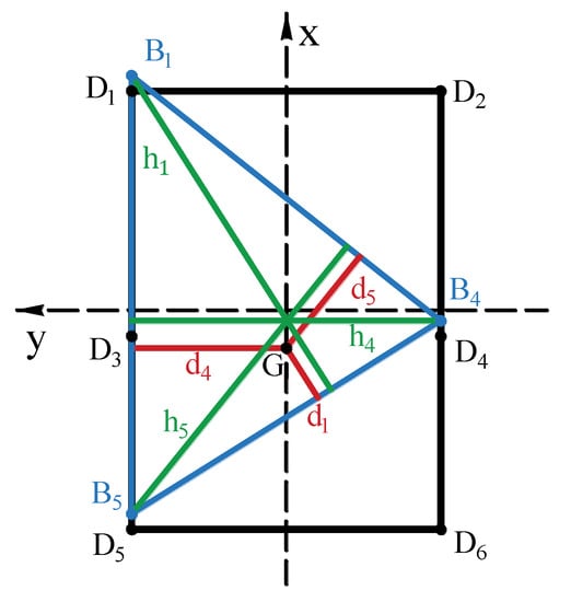
Figure 6.
Supporting point of the HHR.
Taking the robot body’s center projection as the origin of coordinate and the forward direction as the x-axis, the coordinate of the robot body’s barycenter vertical projection is G(n,0) and the vertical projections of root joints are D1(b,a), D2(b,−a), D3(−m,a), D4(−m,−a), D5(−b,a), and D6(−b,−a). Leg (1,4,5) and leg (2,3,6) support the robot alternately, and its supporting force is symmetry in terms of the x-axis. Leg (1,4,5) is applied for calculation.
G is the gravity of the HHR body, and the foot force of leg i (i = 1–6) can be expressed as
where
The joint output torque can be obtained from Equations (10) and (11).
According to Equations (2), (3), and (13), the hydraulic cylinder output force is
3.4. Foot Trajectory Planning Analysis
The straight motion with triangle gait is used to analyze the energy consumption of the HHR. The foot trajectory is designed with a supporting phase and a swing phase: (1) In the supporting phase, the foot contacts the ground and the robot moves at a constant speed; (2) In the swing phase, the foot gets off the ground and swings at a certain height. The swing phase of the foot trajectory is designed based on sextic spline interpolation, and the supporting phase is a straight line. The duty cycle is set to 0.5, and the time of both phases is T/2. When the two phases are switched, it is essential to ensure the continuity of position, velocity, and acceleration of the foot trajectory. The coefficient of the swing phase can be obtained according to the limiting conditions, as shown in Table 2. T is the time cycle of the foot trajectory, H0 is the vertical height of the root joint, si is the offset of the foot trajectory of leg i, and w is lifting height of the foot.
Table 2.
The limiting conditions of the swing phase (0–T/2).
According to the above limits, the foot trajectory can be written in equation, and its curve is shown in Figure 7.
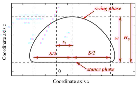
Figure 7.
Foot trajectory curve.
- swing phase (0 < t< T/2)where
- supporting phase (T/2 < t < T)
According to different arrangement of the legs, the coordinate of the foot can be expressed as
3.5. Modeling of Hydraulic Driving System
The HHR is driven by 18 hydraulic cylinders, and the model of a hydraulic driving system for each cylinder is shown in Figure 8. Ps is the pressure of the hydraulic power unit and Pt is the pressure of the oil tank. P1 and P2 are the pressure of the piston and rod chamber, respectively and kq is the gain of the valve. The relationship between the flow rate Q1, Q2, the pressure drop of the valve ΔP, and valve input u can be described by
where
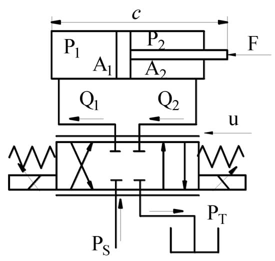
Figure 8.
Hydraulic driving system schematic diagram.
Since the elastic modulus of hydraulic oil is large, and its leakage is few, the flow rate of two chambers can be estimated by the velocity of the piston
where A1 and A2 are the acting area of piston and rod chamber, respectively.
The output force of the hydraulic cylinder can be expressed as
Then P1 and P2 can be derived from Equations (14), (18), (20), and (21):
The length cylinders can be obtained by Equation (1), and their velocity can also be calculated by Equations (2) and (3):
The flow rate of the joint j of leg i provided by the hydraulic power unit can be described as
Considering the contribution of all the joints of the robot, the total energy consumption of the hydraulic driving system can be given by
4. Parameter Optimization
The goal of the optimization problem is to find best solution of the HHR structure and gait parameter under constraints of the geometric and force simultaneously. To ensure the symmetry of the leg structure, there should be a relationship as follows:
The gait of the robot is symmetry, so it should be satisfied that
Thus, the vector of design variables is x = (L1, L2, m, S, φ, a1, b1, e11, e12, s1, s4, s5).
4.1. Objective Functions
For the HHR multi-objective optimization problem, it can be explained by three objectives as follows:
1. Flow rate
According to Equations (25) and (26), the flow quantity of the hydraulic system directly affects the energy of the robot. The minimization of the flow quantity is also significant to reduce the mass of the hydraulic driving system. The quantity of flow is closely related to the robot velocity, so the velocity is set to be constant v = 0.5 m/s. The first objective function can be written as follows:
where is the average flow rate of hydraulic driving system; the period of foot trajectory T is set according to the step length:
2. Maximum pressure
The maximum pressure is the secondary optimization objective. When the robot needs to work in a more complex environment, the system pressure can be adjusted to increase the robot output force. The smaller the maximum pressure, the greater load the robot can increase. Pmax is the maximum pressure of all hydraulic cylinders containing a piston and rod chamber.
3. Minimum stability margin
The third objective function is the stability margin during robot movement, which is designed to increase the motion ability of the robot’s mechanical design. di is the stability margin of leg i (i = 1–6).
To simplify the optimization process, an overall function is adopted by multiplying the three objective functions in exponent. The absolute value of the exponent is the impact factor of the objectives, which means the significance of the objective function. When the impact factor is positive, the goal is to make the objective function as small as possible, and vice versa. The flow quantity directly affects the energy consumption, as the pressure of hydraulic system is set to be 16 MPa. The mass of a hydraulic system is also affected by its flow rate, so λ1 is set as the biggest to determine the leg structure and to reduce the mass of hydraulic system. The maximum pressure Pmax and stability margin are the secondary and third optimization objectives, which are set to increase the motion diversity of the robot’s mechanical design. When the Pmax is smaller than the system pressure, the hydraulic robot can do more difficult movements. The maximization of stability margin can effectively increase the stability under external impact. According to importance, λ2 is set at the middle, and λ3 is set as the smallest. The values of lambda are adjusted by experience that the latter value is half of the previous value for better optimal results. Therefore, the impact factors of the objectives are set as λ1 = 1, λ2 = 0.5, λ3 = −0.25. The overall optimization objective function can be obtained as
4.2. Constraints
From the geometry of the leg structure, limitation of the hydraulic system, and motion stability, a number of non-linear constraints can be derived:
- The distance between the trajectory of the front foot and middle foot should be larger than the allowance, as well as the distance between the trajectory of the middle and hind foot.
- The foot trajectory should be in the foot workspace. Lmax and Lmin are the maximum and minimum length from the hip joint to the foot of all the legs. θ1min, θ1max, θ2min, θ2max are the set angular range for the hip and knee joints.
- When the HHR walks, the stability margin should be greater than zero.
- The pressure of the cylinder chamber should be less than the system pressure and greater than zero.
- The offset of the cylinder should be greater than the allowance.
- The two hydraulic cylinders on the thigh should not interfere with each other. As shown in Figure 3, the distance between the installation point and the other cylinder should be greater than the allowance. is the distance from X3 to the straight line X1 × 2 and is the distance from X2 to the straight line X3X4.
- To ensure the robot’s motion ability, the leg length should be designed to allow the root joint to move 30 degrees sideways without changing its height.
- The arm of force of the hydraulic cylinder affects the control precision, so it should be greater than the allowance.
- The geometric bounds of the design variables.
- The restriction and invariant parameters are assumed to be as a = 280 mm, b = 500 mm, d = 100 mm, a0 = 281 mm, b0 = 67 mm, e01 = 78°, e02 = 52°, n = 0, H0 = 800 mm, w = 10 mm, Ps = 16 MPa, A1 = 491 mm2, A2 = 290 mm2, ε1 = 50 mm, ε2 = 160 mm, ε3 = 45 mm, and ε4 = 40 mm.
4.3. Optimization Result
The genetic algorithm (GA) is an artificial intelligence optimization algorithm for simulating the genetic and evolutionary processes in nature, which owns the characteristics of simplicity and robustness. However, the optimization of the hydraulic legged robot is a highly nonlinear multi-constraint multi-objective problem; the traditional GA cannot form an effective convergence procedure in the HHR optimization process. Archive-based micro genetic algorithm (AMGA) is particularly suitable for solving highly non-linear multi-constraint multi-objective optimizations [34]. The optimizing process of AMGA is shown in Figure 9. The optimization bound for each iteration is set based on the archive of the last iteration, and the parent population is created from the bound. The archive is updated using the optimal solution of each genetic algorithm iteration, which is obtained by selection, crossover, mutation, and sorting. The bound iteration will terminate when the archive does not change. The detail of the mathematical formulation for evaluating the fitness of the off-spring population is given in Appendix A.
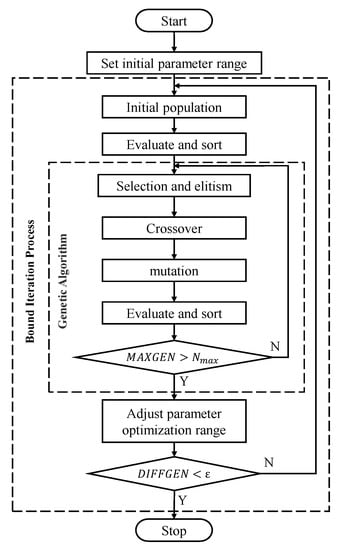
Figure 9.
Flow chart of the archive-based micro genetic algorithm (AMGA) progress.
The bound for each iteration is set as
where xn is the archive of last iteration, MAXGEN is the generation number, DIFFGEN is the difference value between the archive of two iterations, and Nmax is the set generation number.
Figure 10 shows the obtained fitness resulting from the GA and AMGA optimization procedures, which have identical parameter settings, as shown in Table 3. The AMGA generation number for each iteration is 20, and its iteration number is 10. From the fitness curve, we can know that: the traditional GA has a faster convergence rate at the beginning, but the optimization efficiency decreases due to the restrictions of multiple constraints; the AMGA had a limited optimization range for each iteration, but it is more efficient when it gets close to the optimal value.
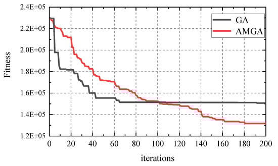
Figure 10.
Evolution of fitness using genetic algorithm (GA) and AMGA.
Table 3.
Identical parameter settings.
The energy consumption of HHR optimization with AMGA is shown in Figure 11. The power of the HHR decreases from 9.32 kW to 5.16 kW. The optimization result is shown in Table 4 and Table 5, which is adjusted after design sensitivity analysis. It can be seen from the specifications that the design of the AMGA value has better performance than the GA. Comparing the initial design with the optimized design of the AMGA value, the power is decreased by 44.6%, with other HHR specifications almost unchanged. It can be seen that the optimized mechanical structure and gait have a great improvement in energy saving, and the correctness of the theoretical calculation is verified in the simulation section.
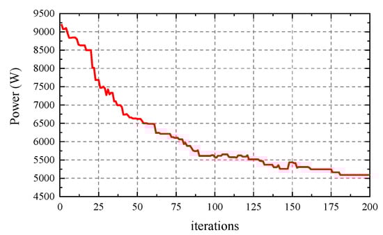
Figure 11.
Evolution of HHR energy consumption with AMGA.
Table 4.
Optimization results.
Table 5.
Specifications of different designs.
4.4. Design Sensitivity Analysis
The design sensitivity analysis provides the derivatives of certain output variables with respect to specified design parameters, which determine the most influential variables on the objective function. The mechanical structure and the gait parameter can be adjusted with the installation and manufacture requirements according to the influence of variables.
It can be obtained as
The magnitude of the sensitivity coefficients indicates the relative importance of that variable on the variation of the objective function. Figure 12 shows the values of the sensitivity coefficients of the objective functions f1(x), f2(x), f3(x), and F(x) on the optimal solution point. Combined with Equations (27) and (28), it shows that the objective function F(x) is most sensitive to the variation of design variables b1 and b2 which influence the arm of force of the actuators, and are limited by the constraints of pressure (Equation (37)), installation position (Equation (39)), and control accuracy (Equation (41)). The value of variables b1 and b2 cannot be decreased. The step length S is the second most important variable and has influence in all objective functions. As the step length increases and the forward speed remains unchanged, the energy consumption of the HHR decreases, the maximum pressure increases, and the stability margin decreases. In the rest variables, L1 and L2 affect the flow rate and maximum pressure of the hydraulic system; m and si (i = 1–6) affect the maximum pressure and motion stability, respectively. Variables a1, a2, e11, e12, e21, e22, and φ have less influence, which can be used for mechanical structure adjustment.
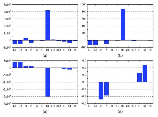
Figure 12.
Design sensitivity for objective function: (a) the overall objective function; (b) flow rate; (c) maximum pressure; (d) stability margin.
5. Simulation and Result Discussion
The HHR performance is tested via the co-simulation of MATLAB/Simulink and ADAMS, which simulate the hydraulic system and robot motion separately, as shown in Figure 13. The mechanical model is established based on the optimization results of AMGA in Table 5, as shown in Figure 14.
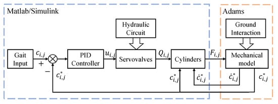
Figure 13.
Overview of the virtual prototype.
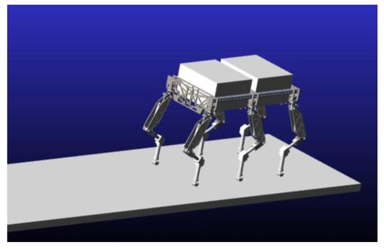
Figure 14.
The mechanical model of HHR in ADAMS.
The servo valve model is approximated by following second-order linear differential equations. ωn is the natural frequency of the servo valve, ξn is the damping ratio, and xi,j* is the servo valve’s spool displacement of the joint j of leg i.
The quantity of flow through the servo valve is established. Qi,j,1* and Qi,j,2* are the flow rate of the piston chamber and rod chamber. Pi,j,1* and Pi,j,2* are the pressure of the piston chamber and rod chamber. fi,j* is the output force of the cylinder. ci,j* is the length of the cylinder.
where
The pressure of the cylinders’ chambers is modeled as
where the volume of the chambers is
The output force of the cylinders transferred to the ADAMS model is
The servo valves are controlled by PID (Proportion-Integral-Derivative) controller with the parameter set as kp = 40, kd = 100, and ki = 0.3, as shown in Equation (50).
Table 6.
The simulation parameters of hydraulic system in MATLAB/Simulink.
Table 7.
The simulation parameters of robot in ADAMS.
From Figure 15 and Figure 16, it can be seen that the cylinder displacement has good control performance in tracking the planning curve, and the HHR proceeds at the expected speed v = 0.5 m/s. Figure 17 shows the simulation curves and theoretical calculation curve for the chamber pressure for the hip hydraulic cylinder of leg 1. The two curves almost coincide with each other except the vibration of the impact stage. The impact was caused by the foot–terrain interaction and errors in the mechanisms and control. The HHR flow rate curve is shown in Figure 18, with its average as 19.47 L/min, and the relative error with theoretical calculation as 0.7%. By multiplying the average flow rate and system pressure Ps, the required power is 5.19 kW. The simulation results agreed well with the theoretical results, and proved that the objective optimization is reasonable and reliable.
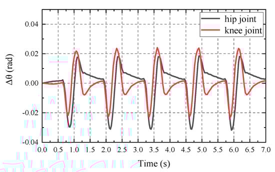
Figure 15.
Tracking error of the leg 1 joints.
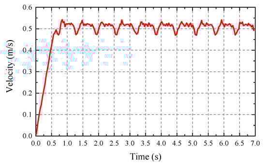
Figure 16.
Forward velocity of the HHR.
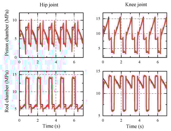
Figure 17.
The cylinder pressure of leg 1.
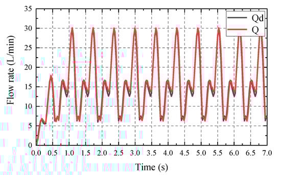
Figure 18.
The total flow rate of the HHR.
6. Conclusions
This paper presents the mechanical design and gait optimization of the hydraulic hexapod robot based on energy conservation. It aims to address the problem of building up a framework for the modeling of the hydraulic walking robot and provides an effective design process based on the proposed framework. A two-stage process was adopted for modeling and optimizing the structural and gait parameters of the HHR. In the modeling stage, a step-by-step study is introduced to build geometric, kinematic, static, foot trajectory, and hydraulic driving system models. By establishing the above model, it is possible to predict the walking state and energy consumption of the robot. The optimization stage shows the procedure to formalize and to solve a highly nonlinear multi-constraint multi-objective optimization. In order to optimize the mechanical structure and gait parameters simultaneously, the objective function contains three parts: flow rate, maximum pressure, and stability margin. Due to the complexity of the problem, the archive-based micro genetic algorithm (AMGA) is applied to find the optimal solution. The AMGA had a limited optimization range for each iteration but is more efficient when it gets close to the optimal value. In the optimal solution, the energy consumption of the HHR reduced 44.6% in comparison with the original mechanical structure and foot trajectory. The virtual prototype based on co-simulation of MATLAB and ADAMS is employed to prove the theoretical result is reasonable and reliable.
Further works in this design process will focus on improving the motion ability of the robot. More operation conditions can be considered and optimized in the gait calculation section, such as turning gait, uphill gait, stair gait, and motion on uneven ground.
Author Contributions
Conceptualization, S.Z., B.J., and Y.C.; methodology, S.Z. and B.J.; software, Y.C.; writing, S.Z.; supervision, B.J. All authors have read and agreed to the published version of the manuscript.
Funding
This work was partially supported by the National Natural Science Foundation of China under grant 51521064 and Ningbo Municipal Bureau of Science and Technology under grant 2019B10052.
Conflicts of Interest
The authors declare no conflicts of interest.
Appendix A. Objective Function for Optimization
| Algorithm A1 Objective function for optimization | Equations |
Require: Design parameter X = (L1, L2, m, S, φ, a1, b1, e11, e12, s1, s4, s5)
| (18) (18)–(20) (8) and (9) (2) (3) (10) and (11) (26) (12) (14) and (15) (16) and (17) (25) (37)–(45) (36) |
References
- Suzumori, K.; Faudzi, A.A. Trends in hydraulic actuators and components in legged and tough robots: A review. Adv. Robot. 2018, 32, 458–476. [Google Scholar] [CrossRef]
- Raibert, M.; Blankespoor, K.; Nelson, G.; Playter, R. Bigdog, the rough-terrain quadruped robot. IFAC Proc. Vol. 2008, 41, 10822–10825. [Google Scholar] [CrossRef]
- Kuindersma, S.; Deits, R.; Fallon, M. Optimization-based Locomotion Planning Estimation and Control Design for the Atlas Humanoid Robot. Auton. Robot. 2016, 43, 429–455. [Google Scholar] [CrossRef]
- Boaventura, T.; Buchli, J.; Semini, C. Model-based hydraulic impedance control for dynamic robots. IEEE Trans. Robot. 2017, 22, 1324–1336. [Google Scholar] [CrossRef]
- Semini, C.; Barasuol, V.; Goldsmith, J. Design of the hydraulically-actuated torque-controlled quadruped robot HyQ2Max. IEEE-ASME Trans. Mechatron. 2017, 22, 635–646. [Google Scholar] [CrossRef]
- Yang, K.; Zhou, L.; Rong, X. Onboard hydraulic system controller design for quadruped robot driven by gasoline engine. Mechatronics 2018, 52, 36–48. [Google Scholar] [CrossRef]
- Huang, Y.; Pool, D.M.; Stroosma, O. Long-Stroke Hydraulic Robot Motion Control with Incremental Nonlinear Dynamic Inversion. IEEE-ASME Trans. Mechatron. 2019, 24, 304–314. [Google Scholar] [CrossRef]
- Davliakos, I.; Roditis, I.; Lika, K. Design, development, and control of a tough electrohydraulic hexapod robot for subsea operations. Adv. Robot. 2018, 32, 477–499. [Google Scholar] [CrossRef]
- Hyon, S.H.; Suewaka, D.; Torii, Y. Design and experimental evaluation of a fast torque-controlled hydraulic humanoid robot. IEEE-ASME Trans. Mechatron. 2016, 22, 623–634. [Google Scholar] [CrossRef]
- Mattila, J.; Koivumäki, J.; Caldwell, D.G. A survey on control of hydraulic robotic manipulators with projection to future trends. IEEE-ASME Trans. Mechatron. 2017, 22, 669–680. [Google Scholar] [CrossRef]
- Yang, H.; Pan, M. Engineering research in fluid power: A review. J. Zhejiang Univ. Sci. 2015, 16, 427–442. [Google Scholar] [CrossRef]
- Ba, K.X.; Yu, B.; Ma, G. A novel position-based impedance control method for bionic legged robots’ HDU. IEEE Access 2018, 6, 55680–55692. [Google Scholar] [CrossRef]
- Koivumäki, J.; Zhu, W.H.; Mattila, J. Energy-efficient and high-precision control of hydraulic robots. Control Eng. Pract. 2019, 85, 176–193. [Google Scholar] [CrossRef]
- Xue, Y.; Yang, J.; Shang, J. Energy efficient fluid power in autonomous legged robotics based on bionic multi-stage energy supply. Adv. Robot. 2014, 28, 1445–1457. [Google Scholar] [CrossRef]
- Du, C.; Plummer, A.R.; Johnston, D.N. Performance analysis of a new energy-efficient variable supply pressure electro-hydraulic motion control method. Control Eng. Pract. 2017, 60, 87–98. [Google Scholar] [CrossRef]
- Zhao, J.; Yang, T.; Ma, Z. Energy Consumption Minimizing for Electro-Hydraulic Servo Driving Planar Parallel Mechanism by Optimizing the Structure Based on Genetic Algorithm. IEEE Access 2019, 7, 47090–47101. [Google Scholar] [CrossRef]
- Rezazadeh, S.; Abate, A.; Hatton, R.L. Robot leg design: A constructive framework. IEEE Access 2019, 6, 54369–54387. [Google Scholar] [CrossRef]
- Ming, M.; Jianzhong, W. Hydraulic-Actuated Quadruped Robot Mechanism Design Optimization Based on Particle Swarm Optimization Algorithm. In Proceedings of the 2011 2nd International Conference on Artificial Intelligence, Management Science and Electronic Commerce (AIMSEC), Dengleng, China, 8–10 August 2011. [Google Scholar]
- Linjama, M.; Huova, M. Model-based force and position tracking control of a multi-pressure hydraulic cylinder. Proc. Inst. Mech. Eng. 2018, 232, 324–335. [Google Scholar] [CrossRef]
- Barasuol, V.; Villarreal-Magaña, O.A.; Sangiah, D. Highly-integrated hydraulic smart actuators and smart manifolds for high-bandwidth force control. Front. Robot. AI 2018, 5, 51. [Google Scholar] [CrossRef]
- Plooij, M.; Wisse, M.; Vallery, H. Reducing the Energy Consumption of Robots Using the Bidirectional Clutched Parallel Elastic Actuator. IEEE Trans. Robot. 2016, 32, 1512–1523. [Google Scholar] [CrossRef]
- Ball, D.; Ross, P.; Wall, J. A novel energy efficient controllable stiffness joint. In Proceedings of the 2013 IEEE International Conference on Robotics and Automation 2013, Karlsruhe, Germany, 6–10 May 2013. [Google Scholar]
- Deng, Z.; Liu, Y.; Ding, L. Motion planning and simulation verification of a hydraulic hexapod robot based on reducing energy/flow consumption. J. Mech. Sci. Technol. 2015, 29, 4427–4436. [Google Scholar] [CrossRef]
- Yang, K.; Li, Y.; Zhou, L. Energy Efficient Foot Trajectory of Trot Motion for Hydraulic Quadruped Robot. Energies 2019, 12, 2514. [Google Scholar] [CrossRef]
- Yang, K.; Rong, X.; Zhou, L. Modeling and Analysis on Energy Consumption of Hydraulic Quadruped Robot for Optimal Trot Motion Control. Appl. Sci. 2019, 9, 1771. [Google Scholar] [CrossRef]
- Gao, H.; Liu, Y.; Ding, L. Low Impact Force and Energy Consumption Motion Planning for Hexapod Robot with Passive Compliant Ankles. J. Intell. Robot. Syst. 2019, 94, 349–370. [Google Scholar] [CrossRef]
- Sumin, P.; Jehyeok, K.; Jay, I.J. Optimal dimensioning of redundantly actuated mechanism for maximizing energy efficiency and workspace via Taguchi method. Proc. Inst. Mech. Eng. Part C J. Mech. Eng. Sci. 2017, 231, 326–340. [Google Scholar]
- Zhu, Y.; Jin, B.; Li, W. Optimal design of hexapod walking robot leg structure based on energy consumption and workspace. Trans. Can. Soc. Mech. Eng. 2014, 38, 305–317. [Google Scholar] [CrossRef]
- Haoyu, R.; Qimin, L.; Bing, L.; Zhenhuan, D. Design and optimization of an elastic linkage quadruped robot based on workspace and tracking error. Proc. Inst. Mech. Eng. Part C J. Mech. Eng. Sci. 2018, 232, 4152–4166. [Google Scholar]
- Ha, S.; Coros, S.; Alspach, A. Computational co-optimization of design parameters and motion trajectories for robotic systems. Int. J. Robot. Res. 2018, 37, 1521–1536. [Google Scholar] [CrossRef]
- Nieto, E.A.B.; Rezazadeh, S.; Gregg, R.D. Minimizing energy consumption and peak power of series elastic actuators: A convex optimization framework for elastic element design. IEEE/ASME Trans. Mechatron. 2019, 24, 1334–1345. [Google Scholar] [CrossRef]
- Sakai, S. Casimir based fast computation for hydraulic robot optimizations. In Proceedings of the 2013 IEEE/RSJ International Conference on Intelligent Robots and Systems, Tokyo, Japan, 3–7 November 2013. [Google Scholar]
- Garcia, E.; Jimenez, M.A.; De Santos, P.G. The evolution of robotics research. IEEE Robot. Autom. Mag. 2007, 14, 90–103. [Google Scholar] [CrossRef]
- Sanagi, T.; Ohsawa, K.; Nakamura, Y. AMGA: An Archive-based Micro Genetic Algorithm for Multi-objective Optimization. In Proceedings of the Conference on Genetic & Evolutionary Computation, Atlanta, GA, USA, 12–16 July 2008. [Google Scholar]
© 2020 by the authors. Licensee MDPI, Basel, Switzerland. This article is an open access article distributed under the terms and conditions of the Creative Commons Attribution (CC BY) license (http://creativecommons.org/licenses/by/4.0/).