Optimization Design of a 2.5 Stage Highly Loaded Axial Compressor with a Bezier Surface Modeling Method

Abstract

Due to the complexity of the internal flow field of compressors, the aerodynamic design and optimization of a highly loaded axial compressor with high performance still have three problems, which are rich engineering design experience, high dimensions, and time-consuming calculations. To overcome these three problems, this paper takes an engineering-designed 2.5-stage highly loaded axial flow compressor as an example to introduce the design process and the adopted design philosophies. Then, this paper verifies the numerical method of computational fluid dynamics. A new Bezier surface modeling method for the entire suction surface and pressure surface of blades is developed, and the multi-island genetic algorithm is directly used for further optimization. Only 32 optimization variables are used to optimize the rotors and stators of the compressor, which greatly overcome the problem of high dimensions, time-consuming calculations, and smooth blade surfaces. After optimization, compared with the original compressor, the peak efficiency is still improved by 0.12%, and the stall margin is increased by 2.69%. The increase in peak efficiency is mainly due to the rotors. Compared with the original compressor, for the second-stage rotor, the adiabatic efficiency is improved by about 0.4%, which is mainly due to the decreases of total pressure losses in the range of above 30% of the span height and 10%–30% of the chord length. Besides, for the original compressor, due to deterioration of the flow field near the tip region of the second-stage stator, the large low-speed region eventually evolves from corner separation into corner stall with three-dimensional space spiral backflow. For the optimized compressor, the main reason for the increased stall margin is that the flow field of the second-stage stator with a span height above 50% is improved, and the separation area and three-dimensional space spiral backflow are reduced.

1. Introduction

Military and civil gas turbine engines can be used for turboshaft engines, drones, missiles, auxiliary power units for large engines, and many more industrial applications. To decrease the energy consumption of gas turbine engines and meet the environmental constraints, higher requirements are put forward for the efficiency of the engine components [1]. The axial compressor is the main consumer of the energy produced by the gas turbine engines and an important component to provide the necessary pressure ratio to the combustion chamber. Therefore, the design requirements of axial compressors are moving towards highly loaded, highly efficient, and large stall margins. For decades, scholars from various countries and institutions have devoted themselves to engineering design to make compressor operation more efficient and have formed an engineering design process that combines one-dimensional analysis, two-dimensional calculation, and three-dimensional computational fluid dynamics (CFD) analysis. However, due to the complexity of the flow field of axial compressors, designing a compressor with highly loaded, highly efficient, and large stall margins is very challenging. Many engineering-design philosophies have emerged over the years. Hatch et al. [2] proposed that the simplified radial balance equation in the design process of compressors is inaccurate. The radial entropy gradient of the compressor should be considered to obtain a correct velocity distribution. Reynolds et al. [3] designed and tested a three-stage axial compressor with various aerodynamic design philosophy concepts: for example, customizable rotor airfoils to reduce shock wave losses, an efficient variable inlet guide vane geometry, a variable stator hub profile to minimize gap losses, and so on. To predict the span-wise parameter and speed line more accurately, Hu et al. [4] proposed a new streamline curvature method to improve the incidence models and loss characteristics, which is mainly used in modern axial transonic compressors. Attia et al. [5,6] developed a new vortex solution for the preliminary design of the axial compressor. This takes into account the distribution of axial and circumferential velocities near the end wall, thereby achieving the purpose of improving the performance in the preliminary design period.

Subsequently, in order to further improve the performance of axial compressors, many scholars introduced optimization technology into the aerodynamic design of axial compressors. Among them, geometric modeling and optimization algorithms are important topics of research. In the field of geometric modeling, the traditional modeling methods are to change the element blade profile of different span-wise sections and change the three-dimensional stacking characteristic. Koller et al. [7] used two third-order spline functions to construct the pressure and suction surfaces, with the leading edge geometry consisting of an ellipse and the trailing edge being described by a circular arc. Oyama et al. [8] used the third-order B-spine curves to change the thickness distribution in different span sections and the mean camber line, thereby improving the efficiency of NASA rotor 67. Astrua et al. [9] adopted another element blade modeling method, which used nondimensional parameterization for the suction and pressure surface, which makes the designer able to change the overall suction or pressure surface with little geometric freedom. The three-dimensional stacking characteristic of the axial compressor mainly includes the sweep and dihedral technology. Gummer et al. [10] applied sweep and lean comprehensively to the booster stator of the BR710 engine, which improved the aerodynamic performance of stators and delayed the occurrence of corner stall. Gallimore et al. [11,12] first successfully reported that the modifications of sweep and lean of the rotor blades in a multistage compressor in the open literature. It achieves the design goal of improving efficiency without significant loss in surge margin. Shahpar et al. [13] used the B-spline curve interpolation to change the three-dimensional stacking law of the compressor rotor rotor37. After optimization, the adiabatic efficiency was improved by 1.28%. Hanan et al. [14] found an optimized sweep stator which is beneficial for decreasing the total pressure loss at the hub region and improving the performance of a multistage axial-flow compressor. Denton et al. [15] systematically expounded the influence mechanism of three-dimensional stacking on axial compressors. It is proposed that the forward-sweep in the tip region of a transonic rotor can significantly improve the stall margin. Besides, designers can reduce losses by changing the distribution of reaction in the span height to avoid applying too much or too little reaction to the hub region. In 2003, Burguburu et al. [16] proposed a novel geometric modeling method. This method uses the Bezier surface method to modify the suction surface of an axial compressor rotor and uses a Navier-Stokes code coupled to the gradient method to improve efficiency by moreover 1% with little change in operating range. Later, Dutta et al. [17] proposed a quasi-3D aerodynamic design concept for blade modeling. In this study, the Bezier surface was chosen to parameterize the camber line angle distribution in the radial direction of the blade along the chord length from the leading edge to the trailing edge. The geometric blades are formed by superimposing the camber line with a given thickness distribution, thereby ensuring a smooth blade shape with few design parameters. In the field of optimization algorithms, Sanger et al. [18] in 1983 first integrated numerical optimization technology with the aerodynamic design of a compressor blade, and successfully used the local optimization algorithm of Control Program for Engineering Synthesis (COPES) to improve the aerodynamic performance of a controlled diffusion airfoil. Subsequently, Kusters et al. [19] optimized and tested several compressor cascades by using an inviscid/viscous two-dimensional flow solver with the normal distribution random search and the gradient method. It reduces the losses of airfoils and widens the range of available incidences. Benini et al. [20] used a multi-objective evolutionary algorithm and the Pareto optimal concept to optimize the compressor rotor with a higher pressure ratio and higher efficiency than those of the original rotor. Yi et al. [21] used the genetic algorithm and response surface model for global optimization to obtain an optimized design of the NASA rotor37, where the adiabatic efficiency was increased by 1.58%.

However, the aerodynamic design and optimization of a high loaded axial compressor with high aerodynamic performance still have three problems, which are rich engineering design experience, high dimensions, and time-consuming calculations. To overcome these three problems, this paper takes an engineering-designed 2.5-stage highly loaded axial flow compressor as an example to introduce the design process and the adopted design philosophies. Then, this paper verifies the numerical method of computational fluid dynamics. A new Bezier surface modeling method for the entire suction surface and pressure surface of blades is developed, and the multi-island genetic algorithm is directly used for further optimization. The new Bezier surface modeling method and the multi-island genetic algorithm greatly overcome the problem of high dimensions and time-consuming calculations. Finally, this paper reveals the internal complex flow mechanism of the peak efficiency and stall margin of the axial compressor before and after optimization.

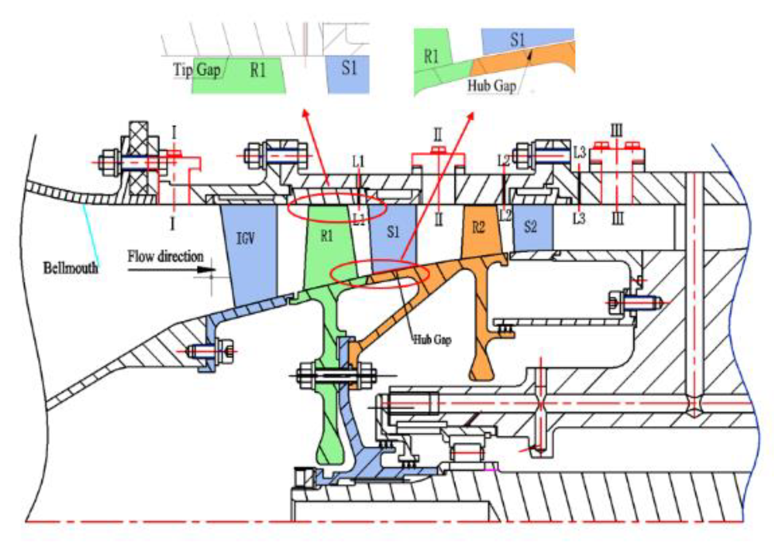
2. Investigated Compressor

The compressor studied in this paper was a 2.5-stage highly loaded axial compressor. It was designed and tested by in the Laboratory of Light-duty Gas-turbine, Institute of Engineering Thermophysics, as shown in Figure 1. It is mainly used in small turbomachinery. The compressor was designed to produce a total pressure ratio of 2.7 at the designed mass flow rate of 4.6 kg/s with an adiabatic efficiency of 86.5%. The key aerodynamic and geometrical parameters of the axial compressor are presented in

Table 1. Key aerodynamic and geometric parameters of the 2.5-stage highly loaded compressor.

Parameter	Symbol	Value
Design total pressure ratio	${\pi }_{td}$	2.7
Design mass flow rate (kg/sec)	$m_d$	4.6
Design adiabatic efficiency	${\eta }_d$	0.865
Design rotational speed (rpm)	$n_d$	25,000
Design rotor tip speed (m/s)	$V_{cd}$	361
Casing diameter (mm)	$D_c$	276
Rotor tip gap (mm)	$G_r$	0.2
Stator hub gap(mm)	$G_s$	0.15
Inlet hub-tip radius ratio	$R_h/R_c$	0.72
Blade numbers	N	31,36,59,45,69
Tip stage loading coefficient	${\psi }_c$	0.46,0.37
Power(kw)	p	500

.

In the preceding literature, various compressor design theories were briefly highlighted. The 2.5-stage highly loaded compressor is engineering designed based on a commercial software Concept AxCent for three-dimensional blade design. The simplified schematic diagram of the design process is shown in Figure 2. To achieve the design goal, several engineering design philosophies were used. Multiple circular arc rotor profiles and bow stators with large turning angle were used to avoid the scale range flow separation. Among all, the three-dimensional CFD calculation is the core of the design process. More design details can be found in the literature [22]. Below, the numerical simulation is introduced in detail.

3. Numerical Simulation

3.1. Numerical Methods

Three-dimensional steady numerical simulation and flow analysis were carried out using the commercial code EURANUS (European Aerodynamic Numerical Solver). This code is an integral part of the software NUMECA FINE. The one-equation Spalart-Allmaras turbulence model was used for the calculations. The Reynolds-averaged Navier–Stokes equation method is still the most widely used approach in industrial CFD due to the computational cost and the design schedule. The spatial treatment of the RANS equations was performed using Jameson’s cell-centered explicit finite volume. Time integration was performed using a four-step Runge-Kutta configuration. To speed up convergence to steady-state, local time stepping, residual smoothing, and multi-grid techniques were all applied. In the computation, the fluid is air modeled as an ideal gas. At the inlet boundary, uniform standard total pressure (101,325 Pa) and total temperature (288.15 K) with axial flow direction were imposed. At the subsonic outlet under the peak efficiency condition, the average static pressure was applied (259,000 Pa). At solid boundaries, i.e., hub, blade, and casing surfaces, adiabatic non-slipping conditions were imposed. A single blade passage was used for the calculations, using periodic boundaries to account for the number of blade passages. A mixing plane was chosen for the rotor-stator interface. The maximum number of iteration steps was set to 1000. The convergence global root mean square residual was set to 1 × 10⁻⁶ to ensure the correct simulation results, the difference between the inlet and outlet calculation mass flow rate was less than 0.01%. All the numerical simulations were started at the choked condition and then marched towards near stall condition with a gradual increase in the average outlet pressure. The predicted near stall point was judged to be the last stable condition before the oscillation in the flow parameters and numerical divergence with increasing iteration numbers. To quantitatively analyze the compressor stability, the stall margin is defined as follows [23]:

$$\mathrm{SM}=\left(\frac{{\pi }_{ts}\ast m_d}{{\pi }_{td}\ast m_s}-1\right)\times 100\%$$

where ${\pi }_{td}$, $m_d$, ${\pi }_{ts}$, and $m_s$ correspond to total pressure ratio at the design point, mass flow rate at the design point, total pressure ratio at near stall point and mass flow at near stall point, respectively.

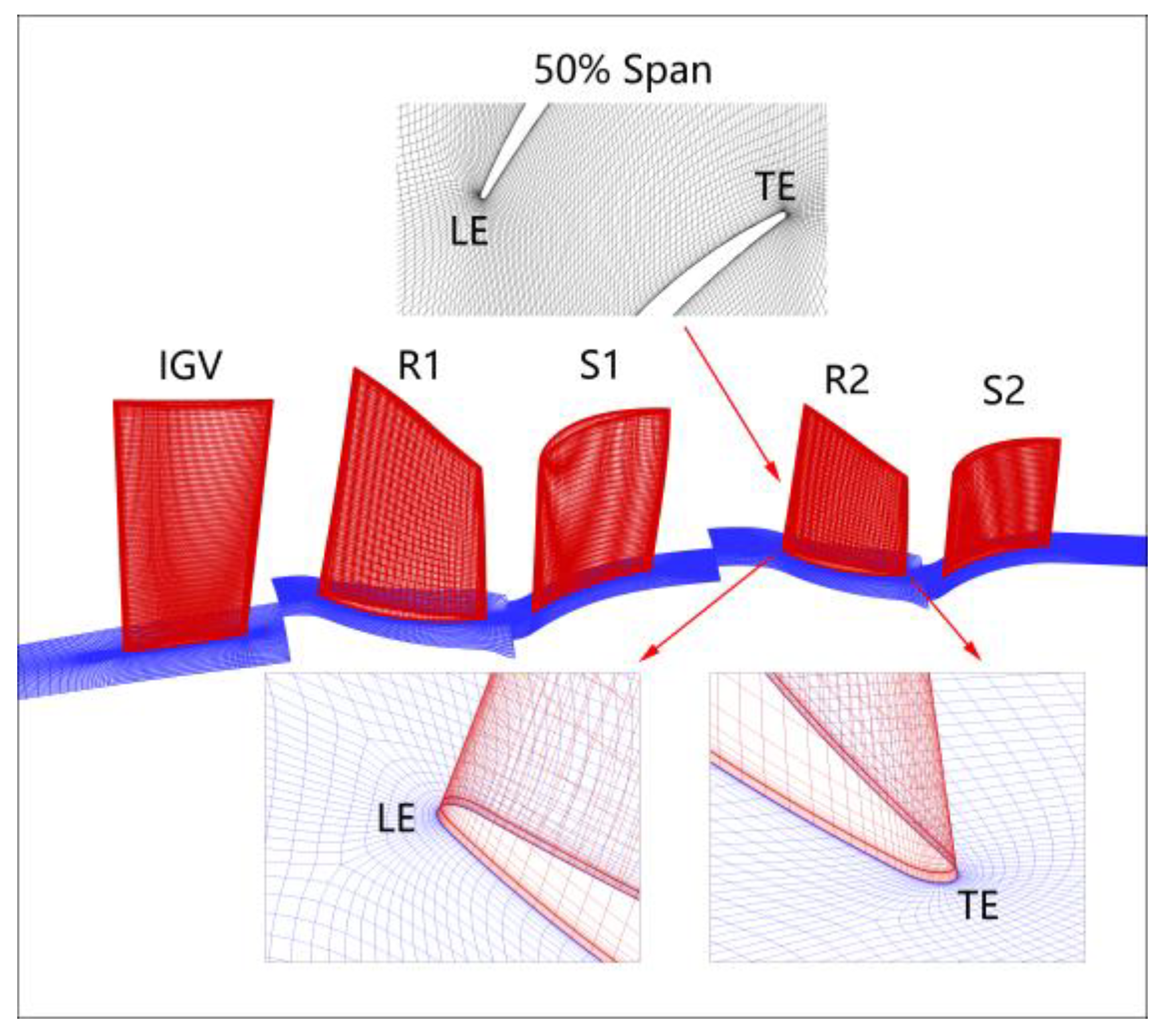
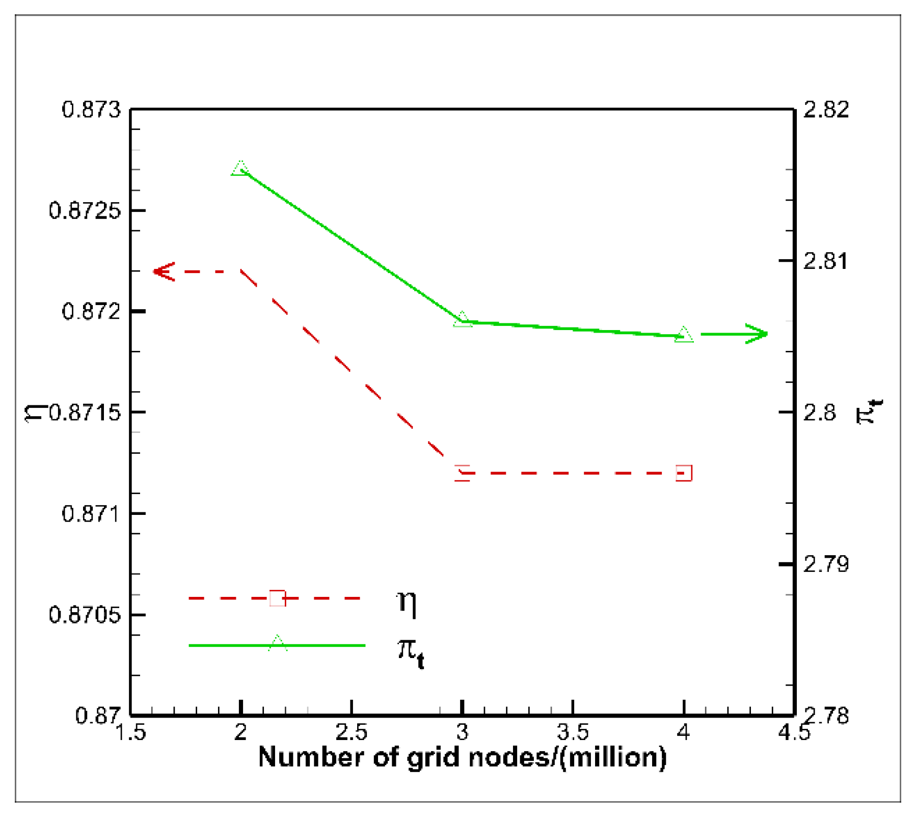
3.2. Grid Topology and Verification

Blade geometry creation and grid generation for the 2.5-stage axial compressor were conducted by using commercial software NUMECA Autogrid 5. Since the grid topology of each blade row is almost similar, this paper describes the grid topology of the second rotor in detail. Multi-block structured grids with hexahedral elements were used in the simulation. Around blade surfaces, the O grids were generated to improve the orthogonality, whereas H grids were used at the inlet, the passage, and the outlet. The distance between the first grid cell and the solid wall was set as 1 × 10⁻⁶ m to meet the need of the solid wall y + < 3 for all computations. Figure 3 shows a single passage for the highly loaded compressor.

To conduct grid independence to eliminate the influence of the number of grid nodes on the flow solution, three different numbers of grid nodes were used to calculate the predicted adiabatic efficiency and total pressure ratio. As can be seen in Figure 4, the adiabatic efficiency and total pressure ratio change slightly from three million grid nodes to four million grid nodes. It means that the number of grid nodes per blade passage was set to three million, which satisfies the requirement of grid independence in the steady-state simulation.

The 2.5-stage highly loaded axial compressor test rig was built at the Institute of Engineering Thermophysics, Chinese Academy of Sciences. The test rig was operated in an open cycle. After the bellmouth and honeycomb, the compressor was driven by an 800 kW AC motor to change the rotational speed. The transmission ratio of the gearbox is 1:12. The range of rotational speed after gearbox is from 0 rpm up to 36,000 rpm, which was measured by an electromagnetic transducer with a relative measurement error within ±0.15%. The mass flow rate was measured by the flow tube mounted in the bellmouth inlet duct within a relative measurement error of ±0.5%. To measure the compressor map, the total temperature and total pressure were captured by probes at the inlet and outlet of the compressor. The temperature was measured by thermocouples with a measurement error of ±0.8 ℃. The total pressure was measured by piezoelectric pressure sensors with a relative full-scale measurement error of ±0.2%. At the compressor inlet, the total pressure was measured by three rake pressure probes with five span-wise locations, while the total temperature was measured by three rake pressure probes with three span-wise locations. At the compressor outlet, the total pressure was measured by six rake pressure probes with three span-wise locations, while the total temperature was measured by six rake pressure probes with three span-wise locations.

To verify the effectiveness of the numerical method, Figure 5 compared the data measured from the experiments and the results from the numerical calculation. The abscissas represented the dimensionless mass flow, which was normalized by the design mass flow. It can be seen that at the 80%, 90% and 100% design speed, the performance maps show the same trend in the adiabatic efficiency and total pressure ratio. For 100% design speed, the total pressure ratios and the peak efficiency in the numerical calculations were almost the same as the experimental value, but when the flow rate was lower than the peak efficiency point the adiabatic efficiency values were higher than the experimental value. The discrepancy of the efficiency maybe since the selected RANS simulation fails to predict the total temperature distribution close to the stall conditions (as shown in the literature [23], which usually occurs in axial compressors) or experimental measurement errors. But the direct numerical simulation calculation is computationally expensive, which makes this approach not suitable for engineering calculations. It should be noted that although the numerical calculation results have a numerical error in predicting the stall flow rate, the following optimization results are only compared to the calculation results, so it will not affect the qualitative conclusion. In a word, the numerical model selected in this paper satisfied the calculation accuracy requirements and could predict the performance of the 2.5-stage highly loaded axial compressor for engineering and analyze the flow mechanism.

4. Optimization Methods

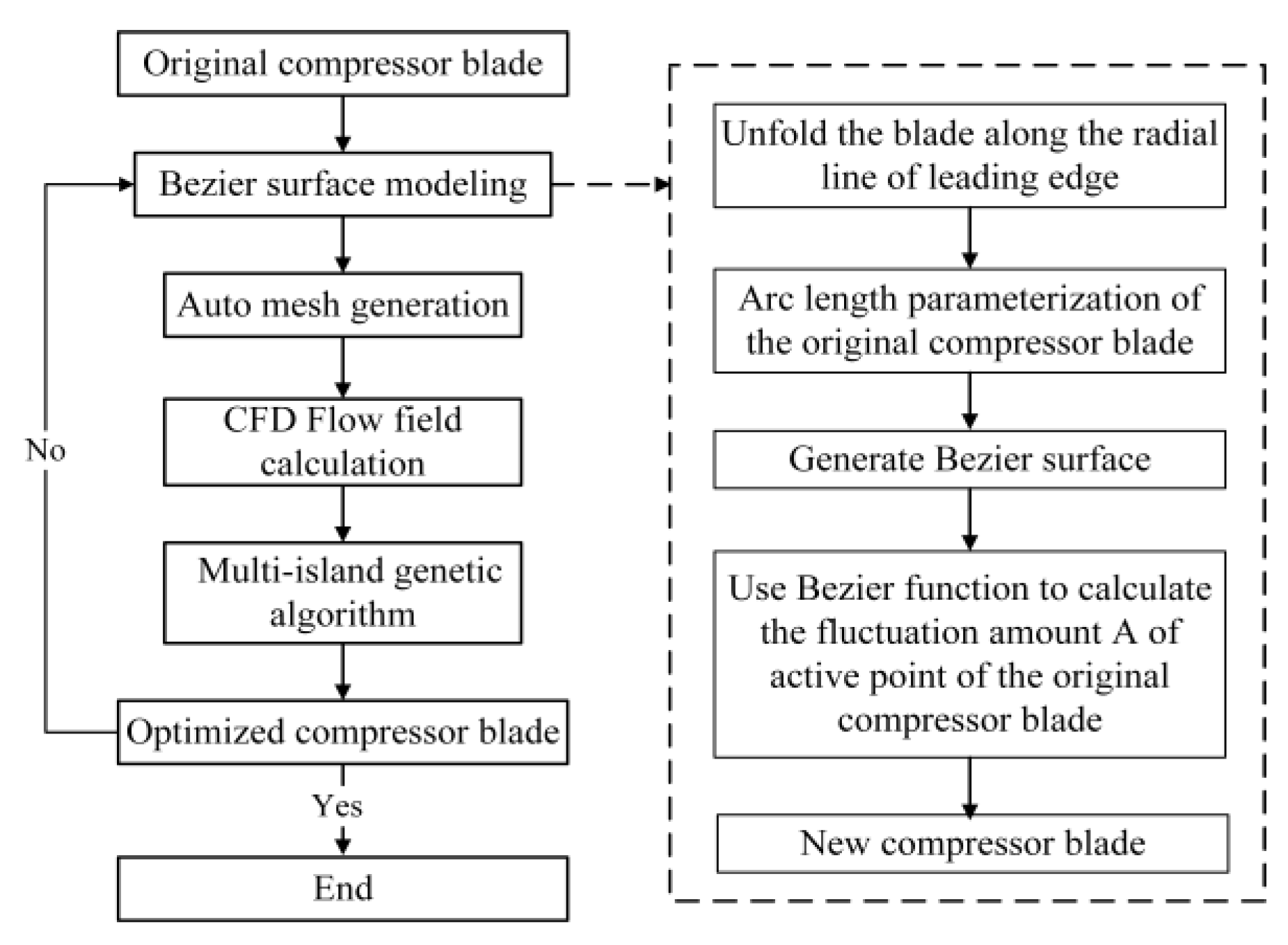
4.1. Bezier Surface Modeling Method

The Bezier surface modeling method means using control points to describe the geometry of the blade. The significant advantage is that the high-order continuity of control points can guarantee the smoothness of the blade surface [16]. This paper first adopts a novel modeling method, as shown in Figure 6, by cutting the compressor blade from the trailing edge, the entire suction surface and pressure surface from a Bezier surface, thereby further reducing the number of design variables. The Bezier surface corresponds to the original blade at the four vertices. The Bezier surface modeling method is to superimpose the Bezier surface based on the original blade by changing the active points.

The process of Bezier surface modeling is divided into two steps. First, the arc length of the original compressor profile is parameterized and converted into the dimensional arc length in the calculation plane. The chord-wise and span-wise directions of the compressor are dimensionless to the unit, respectively. The formula is as follows:

$${\xi }_{i,j}=\frac{{{\displaystyle \sum }}_{m=1}^i{l}_m}{L_j}$$

(1)

$${\gamma }_{i,j}=\frac{{{\displaystyle \sum }}_{n=1}^j{l}_n}{L_i}$$

(2)

where $L_j$ corresponds to the arc length of the radial jth section line; $l_m$ refers to the mth chord length of the radial jth section line; ${\mathsf{\xi }}_{i,j}$ is the dimensionless horizontal coordinates;$L_i$ corresponds to the arc length of the radial ith section line, $l_n$ is the nth chord length on the radial ith section line;${\gamma }_{i,j}$ is the dimensionless ordinate coordinates.

Second, based on the original compressor profile, the Bezier function is used to apply the fluctuation amount A. The value of fluctuation amount A in the circumferential direction is assigned to the original blade to obtain an optimized blade on the calculation plane. The formula is as follows:

$$A={\displaystyle \sum }_{k=0}^n\left\{{\displaystyle \sum }_{l=0}^m{P}_{k,l}{B}_l^m\left(v\right)\right\}{B}_k^n\left(u\right)$$

(3)

$$B_l^m\left(v\right)=C_k^n{v}^l{\left(1-v\right)}^{l-m}$$

(4)

$$B_k^n\left(u\right)=C_k^n{u}^k{\left(1-u\right)}^{n-k}$$

(5)

$$C_k^n=\frac{n!}{\left(n-k\right)!k!}0\le k\le n$$

(6)

In the Formula (3), $P_{k,l}$ corresponds to the control points of the Bezier surface, as can be seen in Figure 6; $B_l^m\left(v\right)$, $B_k^n\left(u\right)$ correspond to Bernstein functions determined by the Formulas (4) and (5), respectively. The v and u are two coordinate axes of the Bezier surface calculation plane; $C_k^n$ is the combinatorial number determined by the Formula (6).

The traditional aerodynamic optimization of the compressor mainly changes the different span-wise profile and three-dimensional sweep-lean characteristics of compressors, resulting in too many design variables, increased design space, and too much calculation cost, which leads to a “dimensional disaster.” It does not meet the actual fast application of the engineering project, thus the optimization fails. In this paper, in order to decrease the number of design variables, the Bezier surface modeling method was selected to optimize the suction surfaces and pressure surfaces of rotors and stators of the compressor, and the 6 × 3 order Bezier surface was used for modeling. According to the engineering philosophy of repeated-stage design, the design variables are further reduced. The fluctuation amount A of the second-stage is the same as the first stage, and the fluctuation amount A of rotors and stators are optimized respectively. The amplitude of fluctuation amount A is plus or minus 2 mm, considering that the geometric changes near the leading edge and the trailing edge have a greater impact on the flow field than the middle chord. Then set seven control points in the direction of ξ (that is, the horizontal coordinate): the positions are 0%, 10%, 30%, 50%, 70%, 90%, and 100% of dimensionless chord length, respectively. Set four control points in the γ direction (that is, the ordinate coordinate) to 0%, 20%, 50%, and 100% of the dimensionless span direction, respectively. The red dots in Figure 7 represent the active control points that can be changed independently. The green dots are located near the leading edge, and the control points have the same magnitude of change in the same span-wise position to avoid discontinuous near the leading edges. Therefore, only 16 active points of each blade row are optimization variables. The 2.5-stage compressor has 32 design variables, which greatly reduces the calculation cost.

4.2. Optimization Process

In this paper, the Isight optimization design platform software is used to build a visual optimization platform under the supercomputing Linux system. Automated optimization is achieved through the C language batch code and Isight Simcode plugin. Due to the objective function of optimization problems encountered in engineering being generally non-linear, the design space has characteristics of being discontinuous and non-linear. The traditional solutions that can be adopted are: adjoint method and surrogate model. The adjoint algorithm is essentially a gradient algorithm, which is easy to fall into local optimal value and cannot find the global optimal value. Thus the reliability of solving the aerodynamic problem of the multi-stage axial compressors is low [24,25,26]. The essence of the surrogate model is to establish a functional relationship between input and output. The disadvantage is that as the variables increase, the number of training samples and the calculation costs increase, and the accuracy deteriorates [27,28,29]. In this paper, the multi-island genetic algorithm (MIGA) is used for optimization. MIGA is a kind of parallel genetic algorithm. It divides the population of individuals into several sub-populations called “islands.” In the MIGA. each population of individuals is altered via the genetic operations of “selection,” “crossover,” and “mutation.” Each design of a population is then evaluated, and its fitness value is determined. All traditional genetic operations are performed separately on each sub-population. Then some individuals are selected from each island and migrated to different islands periodically, which is called “migration.” The parameters of the MIGA are set as follows: the sub-population size and number of generations are set to 10. The mutation rate and the migration rate are set to 0.01. The crossover rate is set to 1 and the migration interval is set to 5. More detail on the MIGA can be found in the literature [30,31,32]. It overcomes the premature convergence problem of traditional genetic algorithms by increasing the diversity of samples, and has a stronger multi-peak searching ability and global optimization capabilities. According to the engineering experience, the peak efficiency point below the design point flow rate is used as an optimization condition to improve the adiabatic efficiency and the surge margin of the original compressor simultaneously. The constraint is that the change in mass flow and total pressure ratio does not exceed 0.5%. The objective function f in the optimization process was set as follows:

$$\max f=\eta \mathrm{if}\{\begin{array}{l}\left|\frac{{\pi }_t-{\pi }_t{}^{Ori}}{{\pi }_t{}^{Ori}}\right|\le 0.5\%\\ \left|m-m_{ori}\right|\le 0.5\%\end{array}$$

(7)

where $\eta$,${\pi }_t$, and $m$ correspond to the adiabatic efficiency, the total pressure ratio of the optimized compressor, the mass flow of the optimized compressor, and${\pi }_t{}^{Ori}$, $m_{ori}$ are the total pressure ratio of the original compressor and the mass flow of the original compressor, respectively.

The whole optimization process of the highly loaded compressor is shown in Figure 8. First, the modeling program reads the geometric information of the original compressor and then generates the Bezier surface modeling of the compressor blade, automatically generating the mesh to perform the three-dimensional CFD flow field calculation. Then, multi-island genetic algorithm optimization is performed to calculate the fitness; that is, the value of the objective function. If the condition for exiting the loop is reached (that is, the global optimal solution is found or the upper limit of the number of iterations is reached), then the optimization is completed and the optimized compressor is the output. Otherwise, the multi-island genetic algorithm will continue to optimize the exploration until the maximum feasible solution of the objective function is searched, thereby obtaining the final optimized compressor blade. The single node of supercomputer used to run the optimization process has an AMD EPYC 7425 2.35 GHz processor, 64 parallel CPUs, and 256 GB RAM. Within the acceptable engineering time requirements, each case takes approximately 8 min and a total of 900 cases are calculated, which takes five days.

5. Results and Discussions

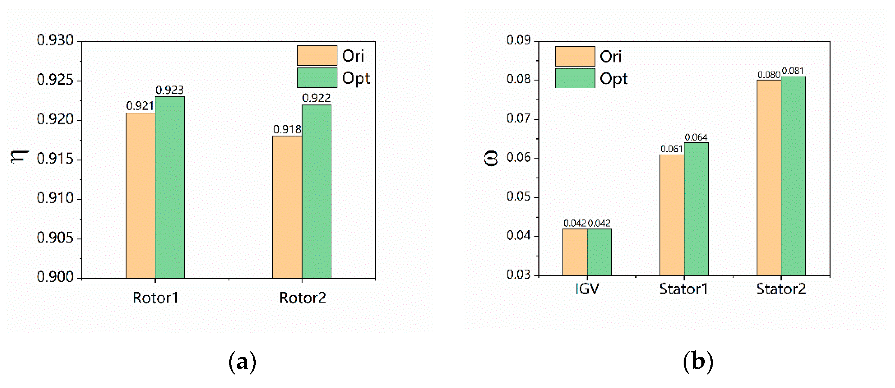
5.1. Analysis of the Optimization Results

Figure 9 shows the original and optimized compressor performance maps. As can be seen in Figure 9, compared with the original compressor the optimized configuration has a higher stall margin, which is about 2.69% higher than that of the original compressor, and the adiabatic efficiency also improves by 0.12%.

To illustrate the information of the optimized blade geometry relative to the original blade geometry, we take the second-stage rotor and the second-stage stator as examples. Figure 10 shows the variation of the second-stage rotor surface of the optimized compressor relative to the original compressor. Among them, Figure 10a shows a three-dimensional modeling diagram of the original second-stage rotor and the optimized second-stage rotor. Figure 10b shows the circumferential fluctuation amount A of the optimized second-stage rotor compared with the original second-stage rotor, where positive values indicate changes in the circumferential position in the direction of the pressure surface and negative values indicate changes in the circumferential position in the direction of the suction surface. It can be seen that the entire second-stage rotor exhibits a positive value, which means the optimized compressor rotor changes in the circumferential position in the direction of the pressure surface. Among them, the area with the largest amplitude of positive values is concentrated near the leading edge in the hub region. This can also be seen from Figure 10a. Besides, the region from the middle section to the trailing edge has the smallest amplitude of positive values, which means that the curvature near the leading edge is greater than that of the middle section, thus the field structure in chord-wise and span-wise direction may be changed.

Figure 11 shows the variation of the second-stage stator surface of the optimized compressor relative to the original compressor. However, it should be noted that the positive values of fluctuation amount A indicate changes in the circumferential position in the direction of the suction surface and negative values indicate changes in the circumferential position in the direction of the pressure surface. This is just the opposite of the rotors. As can be seen in Figure 11b, the changing trend of the second-stage stator is different from that of the second-stage rotor. The area with the largest amplitude of negative values is concentrated near the leading edge above the 50% span region. It means that the stator has a larger turning angle above the 50% span region; this can also be seen from Figure 11a. More analysis of the structure of the flow field is shown below.

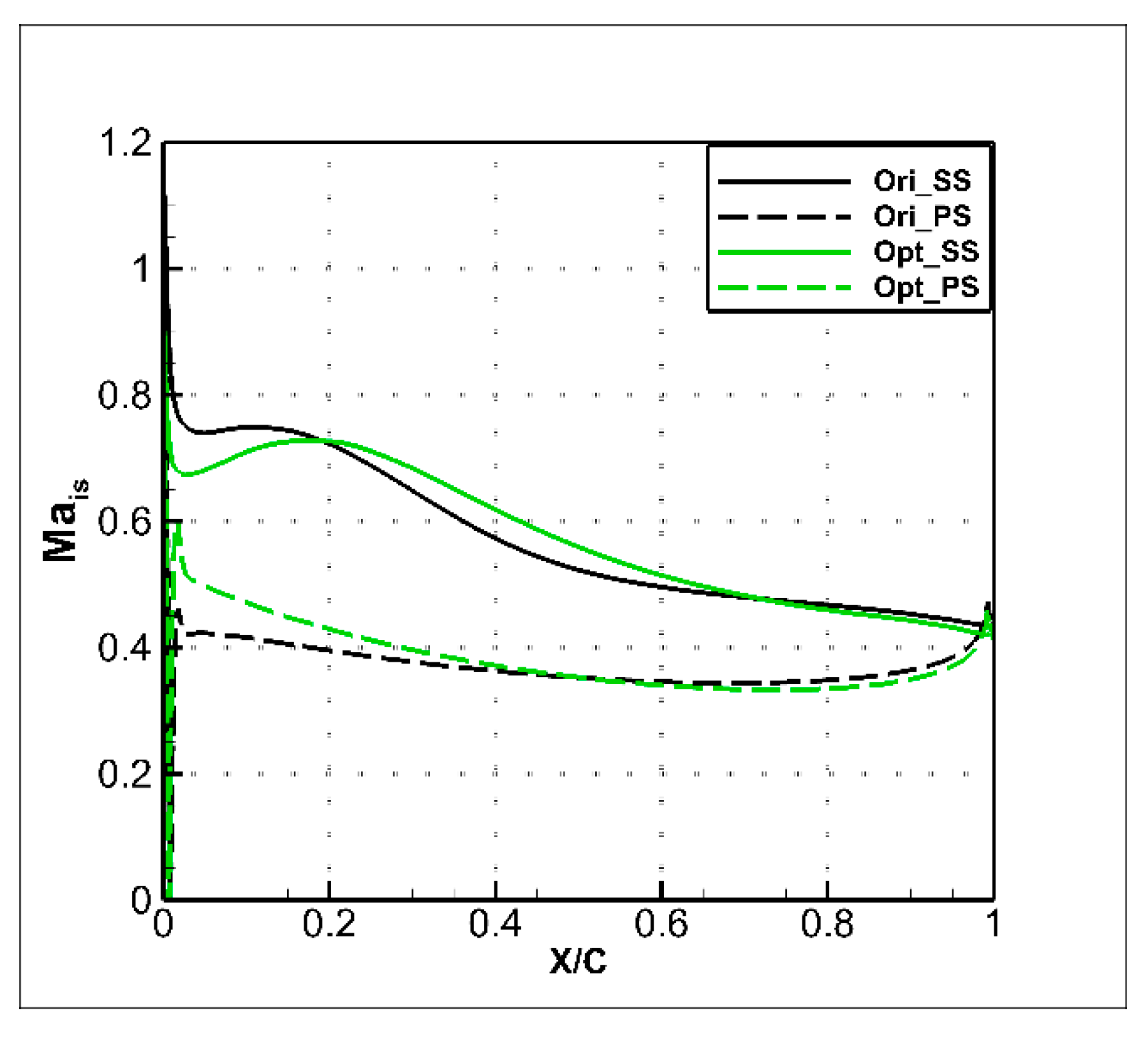
5.2. Discussion on Peak Efficiency Improvement

As shown in Figure 9, the improvement amplitude of the peak efficiency is 0.12%. It also can be seen from Figure 12 that the improvement of the peak efficiency of the highly loaded compressor is mainly due to the improvement in efficiency of rotors. However, the total pressure loss of the stators increases instead. Besides, if we only put the optimization variables on rotors of the original compressor without changing stators, the peak efficiency will be further increased by 0.17% compared with the original compressor, which further supports the trend of efficiency changes. The value of the peak efficiency improvement needs to be further confirmed through experiments. In order to guide the engineering redesign of high loaded compressors, it is worth further analyzing the flow mechanism. In the following, we will focus on analyzing the flow mechanism of the second-stage rotor to improve the peak efficiency of the compressor.

Figure 13 shows the span-wise adiabatic efficiency of the second-stage rotor of the original and optimized compressor. As can be seen in Figure 13, compared with the original rotor the adiabatic efficiency of the optimized rotor above the 30% span height improves, and conversely, the adiabatic efficiency below the 30% span height slightly decreases. This is mainly due to the change of the second-stage rotor of the optimized compressor relative to the original compressor towards the pressure surface, which changes the flow field structure of the second stage rotor in the span-wise and chord-wise direction, as shown in Figure 9. It can be seen from Figure 14 that from the leading edge to 20% of the chord length of the second-stage rotor, the entropy rises rapidly, and then from 20% of the chord length to the trailing edge, the entropy rises gently. Compared with the original compressor, within the range of 10%–30% of the chord length the entropy rise rate of the optimized compressor decreases. Subsequently, the entropy value is always smaller than that of the original compressor. The reasons will be analyzed below.

As shown in Figure 15, after rapid acceleration near the leading edge of the second-stage rotor, the fluid rapidly decelerates along the blade suction surface. Compared with the original rotor, the optimized rotor has a smaller high-speed area range as shown in orange. The fluid decelerates faster and the boundary layer grows more slowly, thus low-energy fluid decreases near the trailing edge. As shown in Figure 16, the isentropic Mach number of the suction surface located at 10% to 30% of the chord length is reduced, which means that the blade loading is reduced, and the change trend of the entropy value shown in Figure 14 is confirmed. Therefore, it indicates that the second-stage rotor of the optimized compressor generates less blade loading and boundary layer losses than that of the second-stage rotor of the original compressor.

5.3. Discussion on Stall Margin Extending

To determine where the stall occurred, we compared the flow fields at different flow coefficients and separately calculated the 1.5-stage and 2-stage compressor flow fields of the original compressor. We found that the compressor can operate at a lower flow coefficient without the second-stage stator, so we infer that the stall of the original compressor occurs in the second-stage stator. From the peak efficiency condition to the near stall condition, when the mass flow decreases the blade loading on the compressor increases. It can be seen in Figure 17 that the flow field near the tip region of the second-stage stator deteriorates and the low-speed region near the trailing edge increases. From Figure 18, we can also find that the fluid separation moves forward on the suction side. Large-scale low-speed areas eventually evolve from small corner separation into corner stall with three-dimensional space spatial backflow.

After optimization, the stall margin of the compressor is increased by 2.69%. To reveal the mechanism of the stall margin improvement, Figure 19 shows absolute Mach number in 95% of the span height of second-stage stator. The near-stall point is chosen for the original compressor, and the same dimensionless flow condition is chosen for the optimized compressor. As shown in Figure 19, compared with the original stator the flow field near the trailing edge region of the optimized second-stage stator in 95% span is improved and the separation region is reduced. As shown in Figure 20, the separation region of the optimized stator moves upstream significantly above the 50% span height. This prevents the occurrence of the corner stall of the second-stage stator and increases the stall margin of the compressor.

However, the study found that at the same normalized mass flow, the inlet swirl angle of the second-stage stator is almost similar, which illustrates the same direction of upcoming flow. The difference of stall margin is in the flow detail of the second-stage stator. Figure 21 shows the isentropic Mach number at the 95% span. It can be seen that the acceleration ability of the fluid near the leading edge on the suction surface of the optimized stator slows down and the peak value of isentropic Mach number slightly decreases. The blade loading is decreased from the leading edge to about 20% of the chord length. The reduced blade loading results in the growth rate of the boundary layer decreases. Finally, the separation region and the three-dimensional spiral backflow decreases. This is mainly as shown in Figure 11, because compared with the original stator the optimized stator has a larger turning angle above the 50% span height. At the same direction of upcoming flow, this means that the incidence is smaller, so the blade loading near the leading edge is smaller and stalls later. Further flow mechanisms, including secondary flows, are worthy of further discussion.

6. Conclusions

Due to the complexity of the internal flow field of axial compressors, the aerodynamic design and optimization of a highly loaded axial compressor with high aerodynamic performance still have three problems, which are rich engineering design experience, high dimensions, and time-consuming calculations. To overcome these three problems, this paper takes an engineering-designed 2.5-stage highly loaded axial flow compressor as an example to introduce the design process and the adopted design philosophies. A new Bezier surface modeling method for the entire suction surface and pressure surface of blades has been successfully applied to the optimization of a highly loaded 2.5-stage axial compressor. Only 32 optimization variables are required, which significantly reduces the number of optimization variables and saves computational costs. Besides, the fine adjustment of the suction surface and the pressure surface of blades can be well achieved, with high smoothness. By using the Bezier surface modeling method the Multi-Island Genetic Algorithm, the aerodynamic performance of the highly loaded transonic 2.5-stage axial compressor is successfully improved. Its advantage is that it can save a lot of calculation costs of engineering design and can quickly and globally optimize the aerodynamic performance of axial compressors. However, its computational costs must be considered in reality, a good engineering design of the compressor is very important.

After optimization, the peak efficiency of the optimized compressor improves by 0.12% compared to the original compressor designed by engineering. The improvement of peak efficiency is mainly due to the rotors. For the second-stage rotor, the adiabatic efficiency improves by approximately 0.4%. Compared with the original compressor, the adiabatic efficiency above 30% of the span height of the optimized compressor improves, and the entropy rise rate within the range of 10%–30% of the chord length of the optimized compressor decreases. For the original compressor, due to the flow field near the tip region of the second-stage stator deteriorating, the large-scale low-speed region eventually evolved from small corner separation into corner stall with the three-dimensional space spiral backflow. For the optimized compressor, the stall margin is increased by 2.69%. The main reason for the increases is that the flow field of the second-stage stator above 50% span height is improved, and the separation region and three-dimensional space spiral backflow are reduced.

References

1. Kalghatgi, G. Development of Fuel/Engine Systems—The Way Forward to Sustainable Transport. Engineering 2019. [Google Scholar] [CrossRef]
2. Hatch, J.E.; Giamati, C.C.; Jackson, R.J. Application of Radial-Equilibrium Condition to Axial-Flow Turbomachine Design Including Consideration of Change of Entropy with Radius Downstream of Blade Row. NASA Clevel. Glenn Res. Cent, USA, RM-E54A20, 1954. Available online: https://digital.library.unt.edu/ark:/67531/metadc60256/ (accessed on 27 April 2020).
3. Reynolds, B.; Etter, S.; Torony, J.; O’Connor, J. Design of a Small Axial Compressor for High Efficiency over a Wide Operating Range. In Proceedings of the ASME 1991 International Gas Turbine and Aeroengine Congress and Exposition, Orlando, FL, USA, 3–6 June 1991. [Google Scholar] [CrossRef] [Green Version]
4. Hu, J.F.; Zhu, X.C.; Ouyang, H.; Qiang, X.Q.; Du, Z.H. Performance prediction of transonic axial compressor based on streamline curvature method. J. Mech. Sci. Technol. 2011, 25, 3037–3045. [Google Scholar] [CrossRef]
5. Attia, M.S.; Li, W. A New Vortex Solution for Axial Compressor Design-Part 1: Design and Methodology. In Proceedings of the AIAA Propulsion and Energy 2019 Forum, Indianapolis, IN, USA, 19–22 August 2019. [Google Scholar] [CrossRef]
6. Attia, M.S.; Li, W. A New Vortex Solution for Axial Compressor Design-Part 2: Validation and CFD Analysis. In Proceedings of the AIAA Propulsion and Energy 2019 Forum, Indianapolis, IN, USA, 19–22 August 2019. [Google Scholar] [CrossRef]
7. Köller, U.; Mönig, R.; Küsters, B.; Schreiber, H.-A. 1999 Turbomachinery Committee Best Paper Award: Development of Advanced Compressor Airfoils for Heavy-Duty Gas Turbines—Part I: Design and Optimization. J. Turbomach. 1999, 122, 397–405. [Google Scholar] [CrossRef]
8. Oyama, A.; Liou, M.-S.; Obayashi, S. Transonic Axial-Flow Blade Optimization: Evolutionary Algorithms/Three-Dimensional Navier-Stokes Solver. J. Propuls. Power 2004, 20, 612–619. [Google Scholar] [CrossRef] [Green Version]
9. Astrua, P.; Piola, S.; Silingardi, A.; Bonzani, F. Multi-Objective Constrained Aero-Mechanical Optimization of an Axial Compressor Transonic Blade. In Proceedings of the ASME Turbo Expo 2012: Turbine Technical Conference and Exposition, Copenhagen, Denmark, 11–15 June 2012. [Google Scholar] [CrossRef]
10. Gümmer, V.; Wenger, U.; Kau, H.-P. Using Sweep and Dihedral to Control Three-Dimensional Flow in Transonic Stators of Axial Compressors. J. Turbomach. 2000, 123, 40–48. [Google Scholar] [CrossRef]
11. Gallimore, S.J.; Bolger, J.J.; Cumpsty, N.A.; Taylor, M.J.; Wright, P.I.; Place, J.M.M. The Use of Sweep and Dihedral in Multistage Axial Flow Compressor Blading—Part I: University Research and Methods Development. J. Turbomach. 2002, 124, 521–532. [Google Scholar] [CrossRef]
12. Gallimore, S.J.; Bolger, J.J.; Cumpsty, N.A.; Taylor, M.J.; Wright, P.I.; Place, J.M.M. The Use of Sweep and Dihedral in Multistage Axial Flow Compressor Blading—Part II: Low and High-Speed Designs and Test Verification. J. Turbomach. 2002, 124, 533–541. [Google Scholar] [CrossRef]
13. Shahpar, S.; Polynkin, A.; Toropov, V. Large scale optimization of transonic axial compressor rotor blades. In Proceedings of the 49th AIAA/ASME/ASCE/AHS/ASC Structures, Structural Dynamics, and Materials Conference, Schaumburg, IL, USA, 7–10 April 2008. [Google Scholar] [CrossRef] [Green Version]
14. Hanan, L.; Li, Q. Analysis and application of a new type of sweep optimization on cantilevered stators for an industrial multistage axial-flow compressor. Proc. Inst. Mech. Eng. Part A J. Power Energy 2015, 230, 44–62. [Google Scholar] [CrossRef]
15. Denton, J.D.; Xu, L. The exploitation of three-dimensional flow in turbomachinery design. Proc. Inst. Mech. Eng. Part C J. Mech. Eng. Sci. 1998, 213, 125–137. [Google Scholar] [CrossRef]
16. Burguburu, S.; Le Pape, A. Improved aerodynamic design of turbomachinery bladings by numerical optimization. Aerosp. Sci. Technol. 2003, 7, 277–287. [Google Scholar] [CrossRef]
17. Dutta, A.K.; Flassig, P.M.; Bestle, D. A Non-Dimensional Quasi-3D Blade Design Approach with Respect to Aerodynamic Criteria. In Proceedings of the ASME Turbo Expo 2008: Power for Land, Sea and Air, Berlin, Germany, 9–13 June 2008. [Google Scholar] [CrossRef]
18. Sanger, N.L. The Use of Optimization Techniques to Design-Controlled Diffusion Compressor Blading. J. Eng. Power 1983, 105, 256–264. [Google Scholar] [CrossRef] [Green Version]
19. Küsters, B.; Schreiber, H.-A.; Köller, U.; Mönig, R. 1999 Turbomachinery Committee Best Paper Award: Development of Advanced Compressor Airfoils for Heavy-Duty Gas Turbines—Part II: Experimental and Theoretical Analysis. J. Turbomach. 1999, 122, 406–414. [Google Scholar] [CrossRef]
20. Benini, E. Three-Dimensional Multi-Objective Design Optimization of a Transonic Compressor Rotor. J. Propuls. Power 2004, 20, 559–565. [Google Scholar] [CrossRef]
21. Yi, W.; Huang, H.; Han, W. Design Optimization of Transonic Compressor Rotor Using CFD and Genetic Algorithm. In Proceedings of the ASME Turbo Expo 2006: Power for Land, Sea and Air, Barcelona, Spain, 8–11 May 2006. [Google Scholar] [CrossRef]
22. Yang, C.; Han, G.; Zhao, S.; Lu, X.; Zhang, Y.; Li, Z. Design and Test of a Novel Highly-Loaded Compressor. In Proceedings of the Turbo Expo: Power for Land, Sea and Air., Phoenix, AZ, USA, 17–21 June 2019. [Google Scholar] [CrossRef]
23. Beheshti, B.H.; Teixeira, J.A.; Ivey, P.C.; Ghorbanian, K.; Farhanieh, B. Parametric Study of Tip Clearance—Casing Treatment on Performance and Stability of a Transonic Axial Compressor. J. Turbomach. 2004, 126, 527–535. [Google Scholar] [CrossRef]
24. Wang, D.X.; He, L. Adjoint Aerodynamic Design Optimization for Blades in Multistage Turbomachines—Part I: Methodology and Verification. J. Turbomach. 2010, 132, 021011. [Google Scholar] [CrossRef]
25. Wang, D.X.; He, L.; Li, Y.S.; Wells, R.G. Adjoint Aerodynamic Design Optimization for Blades in Multistage Turbomachines—Part II: Validation and Application. J. Turbomach. 2010, 132, 021012. [Google Scholar] [CrossRef]
26. Luo, J.; Zhou, C.; Liu, F. Multipoint Design Optimization of a Transonic Compressor Blade by Using an Adjoint Method. J. Turbomach. 2013, 136, 051005. [Google Scholar] [CrossRef]
27. Samad, A.; Kim, K.-Y.; Goel, T.; Haftka, R.T.; Shyy, W. Multiple Surrogate Modeling for Axial Compressor Blade Shape Optimization. J. Propuls. Power 2008, 24, 301–310. [Google Scholar] [CrossRef]
28. Lian, Y.; Liou, M.-S. Multiobjective Optimization Using Coupled Response Surface Model and Evolutionary Algorithm. AIAA J. 2005, 43, 1316–1325. [Google Scholar] [CrossRef]
29. Mengistu, T.; Ghaly, W. Aerodynamic optimization of turbomachinery blades using evolutionary methods and ANN-based surrogate models. Optim. Eng. 2007, 9, 239–255. [Google Scholar] [CrossRef]
30. Wang, W.; Yuan, S.; Pei, J.; Zhang, J. Optimization of the diffuser in a centrifugal pump by combining response surface method with multi-island genetic algorithm. Proc. Inst. Mech. Eng. Part E J. Process. Mech. Eng. 2016, 231, 191–201. [Google Scholar] [CrossRef]
31. Kim, S.; Kim, K.; Son, C. Adaptation Method for Overall and Local Performances of Gas Turbine Engine Model. Int. J. Aeronaut. Space Sci. 2018, 19, 250–261. [Google Scholar] [CrossRef]
32. Jiang, Y.; Lin, H.; Yue, G.; Zheng, Q.; Xu, X. Aero-thermal optimization on multi-rows film cooling of a realistic marine high pressure turbine vane. Appl. Therm. Eng. 2017, 111, 537–549. [Google Scholar] [CrossRef]
Figure 1. Schematic diagram of the 2.5-stage highly loaded compressor.
Applsci 10 03860 g001
Figure 2. Simplified schematic diagram of the design process of the highly loaded compressor.
Applsci 10 03860 g002
Figure 3. Grid topology for the highly loaded compressor.
Applsci 10 03860 g003
Figure 4. Compressor performance with different numbers of grid nodes at the optimization point.
Applsci 10 03860 g004
Figure 5. Calculated and measured compressor performance maps. (a) Adiabatic efficiency at the different normalized mass flow; (b) total pressure ratio at the different normalized mass flow.
Applsci 10 03860 g005
Figure 6. Bezier surface modeling of a compressor blade.
Applsci 10 03860 g006
Figure 7. Bezier surface active control points.
Applsci 10 03860 g007
Figure 8. Optimization process of the highly loaded compressor.
Applsci 10 03860 g008
Figure 9. Original and optimized compressor performance maps. (a) Adiabatic efficiency at the different normalized mass flow; (b) total pressure ratio at the different normalized mass flow.
Applsci 10 03860 g009
Figure 10. Comparison of suction and pressure surface of the original and optimized second-stage rotor. (a) Three-dimensional modeling diagram of the original second-stage rotor and the optimized second-stage rotor; (b) the circumferential fluctuation amount A of the optimized second-stage rotor compared with the original second-stage rotor.
Applsci 10 03860 g010
Figure 11. Comparison of suction and pressure surface of the original and optimized second-stage stator. (a) Three-dimensional modeling diagram of the original second-stage stator and the optimized second-stage stator; (b) the circumferential fluctuation amount A of the optimized second-stage stator compared with the original second-stage stator.
Applsci 10 03860 g011
Figure 12. Rotor adiabatic efficiency and stator total pressure loss of the original and optimized compressor. (a) Rotor adiabatic efficiency at peak efficiency condition; (b) stator total pressure loss at peak efficiency condition.
Applsci 10 03860 g012
Figure 13. Span-wise adiabatic efficiency of the second-stage rotor of the original and optimized compressor.
Applsci 10 03860 g013
Figure 14. Chord-wise entropy rise of the second-stage rotor of the original and optimized compressors.
Applsci 10 03860 g014
Figure 15. Relative Mach number in 70% of the span height of second-stage rotor of the original and optimized compressor. (a) Relative Mach number of the original compressor; (b) relative Mach number of the optimized compressor.
Applsci 10 03860 g015
Figure 16. Isentropic Mach number on 70% of the span height of second-stage rotor of the original and optimized compressor.
Applsci 10 03860 g016
Figure 17. Absolute Mach number in 95% of the span height of second-stage stator from the peak efficiency condition to near stall condition. (a) Absolute Mach number at peak efficiency condition; (b) absolute Mach number at near stall condition.
Applsci 10 03860 g017
Figure 18. Limiting streamline on the suction surface of the second-stage stator from the peak efficiency condition to the near stall condition. (a) Limiting streamline on the suction surface at peak efficiency condition; (b) limiting streamline on the suction surface at near stall condition.
Applsci 10 03860 g018
Figure 19. Absolute Mach number in 95% of the span height of the second-stage stator for original and optimized compressor. (a) Absolute Mach number for original compressor; (b) absolute Mach number for optimized compressor.
Applsci 10 03860 g019
Figure 20. Limiting streamline on the suction surface of the second-stage stator for original and optimized compressor. (a) Limiting streamline on the suction surface for original compressor; (b) limiting streamline on the suction surface for optimized compressor.
Applsci 10 03860 g020
Figure 21. Isentropic Mach number on 95% of the span height of second-stage stator for original and optimized compressor.
Applsci 10 03860 g021