Neural Architecture Search for a Highly Efficient Network with Random Skip Connections

Abstract

Regarding the sequence learning of neural networks, there exists a problem of how to capture long-term dependencies and alleviate the gradient vanishing phenomenon. To manage this problem, we proposed a neural network with random connections via a scheme of a neural architecture search. First, a dense network was designed and trained to construct a search space, and then another network was generated by random sampling in the space, whose skip connections could transmit information directly over multiple periods and capture long-term dependencies more efficiently. Moreover, we devised a novel cell structure that required less memory and computational power than the structures of long short-term memories (LSTMs), and finally, we performed a special initialization scheme on the cell parameters, which could permit unhindered gradient propagation on the time axis at the beginning of training. In the experiments, we evaluated four sequential tasks: adding, copying, frequency discrimination, and image classification; we also adopted several state-of-the-art methods for comparison. The experimental results demonstrated that our proposed model achieved the best performance.

1. Introduction

Sequence learning is a promising field for modeling sequential data [1] and is widely used in time-series predictions, video analysis, information retrieval, etc., where models must learn from sequences, such as those found in speech, documents, videos, etc. Using a recurrent neural network (RNN) has become the standard approach for processing sequential data. Although RNNs have shown remarkable performances in many areas, long-term sequence learning remains challenging due to the gradient vanishing problem. Hence, many improved cell structures have been proposed to manage this problem, such as long short-term memory (LSTM) [2], gated recurrent units (GRUs) [3], and the Just Another Network (JANET) [4]. Others focus on the networks’ architectures, such as, the skip RNN [5], dilated RNNs [6] and hierarchical multi-scale RNNs [7]. However, these networks depend on human design, which demands a lot of expert knowledge and it is usually hard to obtain ideal frameworks. The neural architecture search has emerged for solving this problem, which aims to find good architectures using a controller network, such as an RNN. Investigating neural architecture search (NAS) [8,9] methods has become an important research direction nowadays, which comprises three parts: a search space, a search strategy, and a performance estimation strategy. A search space defines which architecture can be discovered in principle, such as chain-structured neural networks [10]; many different search strategies are used to explore the search space, including random search, evolutionary methods, reinforcement learning, etc.; while performance estimation is used as a feedback to the search strategy. In this paper, we propose to utilize a neural architecture search for managing long-term dependencies in sequential data. First, we designed a dense neural network to construct the search space, which was composed of a novel resource-saving cell structure, and then we selected a network architecture with skip connections via random sampling on the generated probabilities. Next, the architecture was chrono-initialized and trained. The network’s high efficiency lay in three aspects: (1) the remote skip connections directly capture long-term dependencies and can shorten the path length of information propagation; (2) the cell structure demands minimum computational and memory resources compared with other algorithms like JANET; and (3) chrono-initialization can alleviate the gradient vanishing problem along the propagation path.

This paper is organized as follows. Section 2 presents related work. In Section 3, the first part illustrates our proposed method of architecture generation, while the second part presents a special initialization scheme that can capture the dependencies more effectively and alleviate the gradient vanishing problem. Section 4 analyzes the advantages of our network in terms of memory and computational power consumption, and then provides the experimental results. Section 5 gives concluding remarks and prospects for future work.

2. Related Work

For modeling the long-term memory, numerous approaches have been proposed. As mentioned above, some utilize new cell structures, such as the GRU and JANET, which both employ information-latching to alleviate the gradient vanishing problem. Additionally, JANET has achieved good performances by using the least parameters so far. In a JANET cell, only one forgetting gate is preserved and the input gate relies on the forgetting gate, which can save half of the parameters.

Some try to exploit an appropriate initialization scheme of parameters; for instance, Tallec et al. [11] proposed a chrono-initializer that can make the characteristic forgetting time of models lie in approximately the same range as the dependencies in the data sequences, thus the long-term information is much easier to be memorized using a more appropriate initial setting. The chrono-initializer is also adopted in JANET, where the authors demonstrated that the initializing scheme can promote performance when used in their own designed cell structures.

Others adopt alternative neural architectures to shorten the recurrent length [6] and then improve the memory capacity. For instance, a hierarchical recurrent neural network [7] was designed to extract temporal dependencies from multiple time scales by assuming that the dependencies are structured hierarchically; a dilated recurrent neural network [6] was designed to utilize multi-resolution skip connections to learn dependencies in different scales; a phased LSTM [12] applied a time gate controlled by oscillations to update its cell states; and a skip RNN [5] learned to skip state updates at certain times, in which binary gates were trained as an indicator for updating. The former two networks in this category rely on multilayers to capture dependencies at different scales, which tends to incorporate too many parameters, which requires a large amount of memory; the third model produces rhythmic updates of the cell and the last one performs updating on arbitrary time steps, but neither of them can connect the dependencies over remote distances. Thus, in this paper, we propose a neural architecture with remote random connections and provide an optimization scheme based on a neural architecture search.

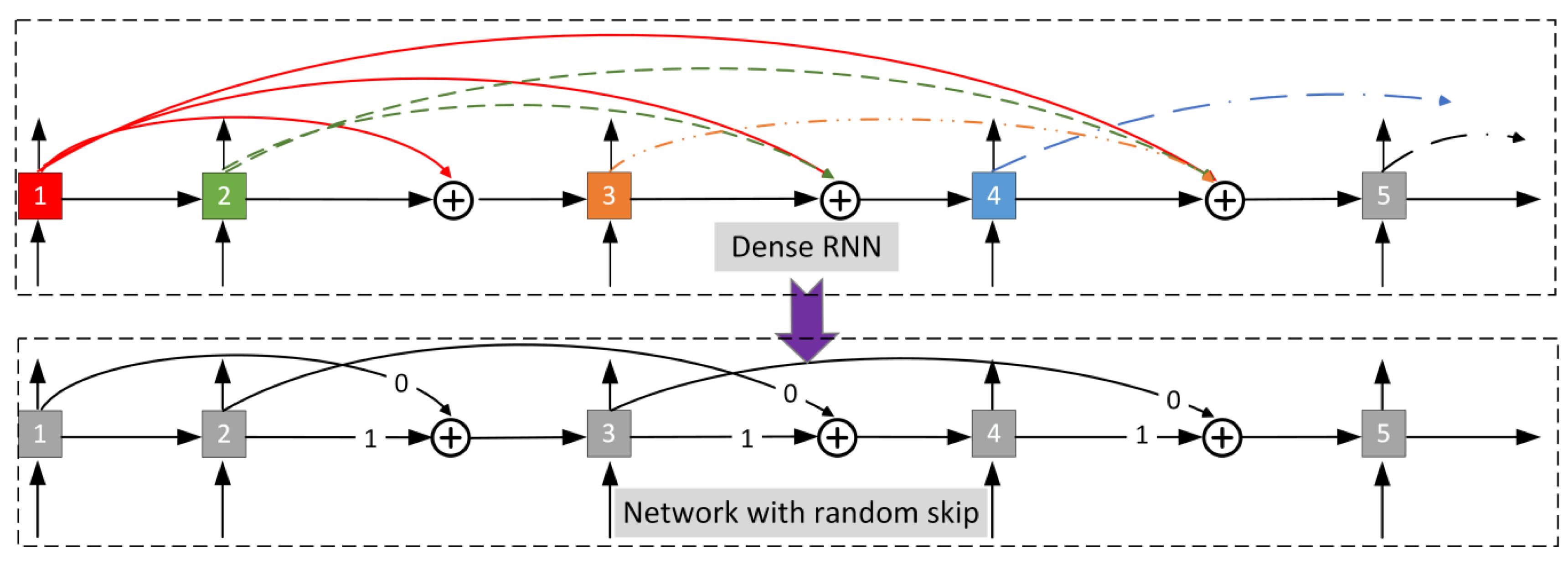
3. A Highly Efficient Network with Random Skip Connections

3.1. Architecture Generation via a Neural Architecture Search

Skip connections across multiple timestamps have been demonstrated to be beneficial for solving the gradient vanishing problem [13,14], but too many remote connections would slow the network’s execution speed down sharply, and unfortunately, it is difficult to select them by hand. Hence, we used a neural architecture search to manage this problem. First, we proposed a dense network that can provide a selection space for the skip connections, where the cell structure is based on that of the standard LSTM [15], which is defined as:

$$\begin{array}{l}{f}_t=\sigma (W_f{h}_t+U_f{y}_{t-1}+b_f)\\ i_t=\sigma (W_i{h}_t+U_i{y}_{t-1}+b_i)\\ g_t=\sigma (W_g{h}_t+U_g{y}_{t-1}+b_g)\\ o_t=\sigma (W_o{h}_t+U_o{y}_{t-1}+b_o)\\ c_t=f_t\odot c_{t-1}+i_t\odot g_t\\ h_t=o_t\odot tanh(c_t)\end{array}$$

(1)

where ${\{\mathrm{f},\mathrm{i},\mathrm{o}\}}_{\mathrm{t}}$ denote the forget, input, and output gates at time t, respectively; $\sigma$ denotes the sigmoid function; ${\mathrm{c}}_t$ represents the cell state; and ${\mathrm{h}}_t$ indicates the output of the hidden layer. Taking the standard meaning, our cell structure can be formulated as:

$$\begin{array}{l}{f}_t=\sigma (W_f{x}_t+b_f)\\ i_t=\sigma (W_i{x}_t+b_i)\\ c_t=f_t\odot \left({\displaystyle \sum _{i=1}^{t-1}}{\omega }_i{c}_i\right)+i_t\odot tanh(W_c{x}_t+b_c)\\ h_t=c_t,\end{array}$$

(2)

where $\sigma$ represents the sigmoid function, ${\mathrm{x}}_t$ is an input vector at t-th time step and ${\omega }_{\mathrm{i}}$ is a combination coefficient. In the cell structure, the forget gate ${\mathrm{f}}_t$ only depends on the inputs at the current timestamp and the input gate ${\mathrm{i}}_t$ only depends on the previous hidden vector, which is different from the standard LSTM; the benefit of this difference is analyzed in Section 4. Moreover, each cell receives state vectors from all of its counterparts at previous timestamps; this architecture consequently forms a dense network. A linear combination of coefficients can be obtained via network training until convergence, where a larger value of ${\omega }_{\mathrm{i}}$ indicates a stronger remote dependency associated with the corresponding skip connection. Thus, it is reasonable to sample one connection and construct a new network. The probabilities of sampling are generated using $\mathrm{soft}\max (\{{\omega }_i|i=1,2,\cdots ,t-2\})$, where the timestamp $\mathrm{t}-1$ is excluded since its corresponding cell will be used in the constructed network.

The framework of this process is depicted in Figure 1 and the auto-generated network is given as:

$$\begin{array}{l}{f}_t=\sigma (W_f{h}_t+b_f)\\ i_t=\sigma (U_i{y}_{t-1}+b_i)\\ c_t=f_t\odot ({\omega }_1{c}_{t-1}+(1-{\omega }_1)c_s)+i_t\odot tanh(W_c{x}_t+b_c)\\ h_t=c_t,\end{array}$$

(3)

where ${\mathrm{c}}_t$ means a sampled state vector. Using this method, the network establishes one remote connection for each cell and is capable of shortening the path length of long-term dependencies. Note that when training the dense network, we can use a small number of hidden units to decrease the dimensions and accelerate the speed because only the dependency relationship needs to be explored. Then, we can use the proper number of hidden units to train the constructed network, which is concentrated on performance improvement.

3.2. Initialization of the Auto-Generated Network

The networks are trained using a gradient backpropagation algorithm to effectively capture the dependencies that Tallec et al. [11] proposed, which use a chrono-initializer in LSTM and GRU cell structures. Here, we adopted the initializer in our designed cell and demonstrate two aspects of theoretical advantages: capturing dependencies and unhindered gradient propagation. We took the auto-generated network as an example, where the coefficients were initialized as ${\omega }_1=1$ such that the cell structure became:

$$c_t={\mathit{f}}_t\odot c_{t-1}+{\mathit{i}}_t\odot tanh(W_c{x}_t+b_c),$$

(4)

which was then considered to be a leaky RNN [12]:

$$c_t=(1-\alpha )\odot c_{t-1}+\alpha \odot tanh(W_c{x}_t+b_c),$$

(5)

where $1-\alpha$ and $\alpha$ represent combination coefficents and should be learned with ${\mathrm{f}}_t$ and ${\mathrm{i}}_t$, respectively. By taking the first-order Taylor expansion [4], we have:

$$\frac{dc(t)}{\mathit{d}t}=-\alpha \odot c(t)+\alpha \odot tanh(W_c{x}_t+b_c),$$

(6)

with the inputs ${\mathrm{x}}_t$ and hidden vectors centered around zero, and ${\mathrm{b}}_c$ initialized to be $0$, we have:

$$\begin{array}{l}\frac{dc(t)}{\mathit{d}t}=-\alpha \odot c(t)\\ {{\displaystyle \int }}_{t_0}^t\frac{1}{c(t)}\mathit{d}c(t)=-\alpha {{\displaystyle \int }}_{t_0}^t\mathit{d}t\\ c(t)=c(t_0)exp(-\alpha (t-t_0)),\end{array}$$

(7)

$\mathrm{c}(t)$ will decrease to ${\mathrm{e}}^{-1}\mathrm{c}(t)$ over a time of $\frac{1}{\alpha }$, which is called the forgetting time and is symbolized as $\mathrm{T}$. Then, the forget and input gates in the auto-generated network should approximate $1-\frac{1}{T}$ and $\frac{1}{T}$, respectively. As $\mathrm{T}$ cannot be known previously, we set:

$$b_f\sim \log (\mu (\left[1,T_{max}-1\right], b_i=-b_f$$

(8)

where $\mu$ represents a uniform distribution. Under the conditions of zero-centered inputs and hidden layers, we have $\sigma (W_f{x}_t+b_f)=\sigma (b_f)\approx 1-\frac{1}{T}$ and $\sigma (U_i{h}_{t-1}+b_i)=\sigma (b_i)\approx \frac{1}{T}$. This means that the forgetting time of our network can lie in approximately the same range as the dependencies of the sequential data.

Moreover, the gradient used for updating one parameter can be formulated as:

$$\begin{array}{l}\frac{\partial J}{\partial U_i}=\frac{\partial J}{\partial c_T}\frac{\partial c_T}{\partial U_i}+\frac{\partial J}{\partial c_T}\frac{\partial c_T}{\partial c_{T-1}}\frac{\partial c_{T-1}}{\partial U_i}+\cdots +\frac{\partial J}{\partial c_T}{\displaystyle \prod _{k=2}^T}\left[\frac{\partial c_k}{\partial c_{k-1}}\right]\frac{\partial c_1}{\partial U_i}\\ \frac{\partial c_t}{\partial c_{t-1}}=\sigma (W_f{x}_t+b_f)+U_i{\sigma }^{\prime }(U_i{h}_{t-1}+b_i)\odot tanh(W_c{x}_t+b_c),\end{array}$$

(9)

where $J$ symbolizes the objective function, $\sigma (W_f{x}_t+b_f)$ approaches 1 when the dependency length $T$ is large, and other items will approximate 0. Thus, we have $\frac{\partial c_k}{\partial c_{k-1}}\approx 1$. In this case, the vanishing gradient can be prevented remarkably well as the multiplication effect is dramatically eliminated; meanwhile, the long-term gradient propagation can be retained.

4. Experimental Results

In this section, we analyze the advantages of our proposed model in terms of memory and computational power first, and then evaluate two kinds of datasets: (1) synthesized data, such as sinusoids and sequences for adding or copying; and (2) public databases, such as the digit dataset of MNIST, which is commonly tested in sequence learning. For the evaluation part, we selected several methods, including those that are the state of the art, for comparison; for instance, the RNN, standard LSTM (abbreviated as sLSTM) [15], JANET [4], Skip GRU [5], Recurrent Neural Network using rectified linear units (iRNN) [16] and Unitary evolution Recurrent Neural Network (uRNN) [17], etc. We cite the results directly if they were presented in the original papers. For the methods run by us, training was performed with an Adam [18] optimizer, a batch size of 200, a learning rate of 0.001, and a gradient clipping [19] threshold of 1. In our model, the dense network was set to have eight units in its hidden layers in all the experiments below since the purpose of this network was to capture the dependencies in the training data and provide a search space; therefore, a limited unit number was sufficient and could guarantee a satisfactory training speed. The unit numbers adopted in the generated network were different and are shown in the testing tasks.

4.1. Benefits Regarding Memory and Computational Power

The use of less computational resources is an important performance criterion for a network. We compared our auto-generated network with the standard LSTM [15] and JANET, which comprises only one forgetting gate and can save resources remarkably well. Assuming the standard LSTM has $n_1$ inputs and $n_2$ hidden units, as declared in Westhuizen and Lasenby [4], the total number of parameters with the LSTM and JANET were $4(n_1{n}_2+n_2^2+n_2)$ and $2(n_1{n}_2+n_2^2+n_2)$, respectively. In our network (see Equation (3)), the numbers were as follows: $f_t$: $n_1{n}_2+n_2$, $i_t$: $n_2^2+n_2$, and others: ${1+n}_1{n}_2+n_2$; therefore, the total number was $n_2^2{+2\mathrm{n}}_1{n}_2+3n_2$. Typically, the values are dominated by the $n_2^2$ term since the hidden units number $n_2$ is usually much larger than the input size $n_1$. The memory requirements lie in approximately the same range as the parameter numbers [4]. As for the computational power, Adolf et al. [20] demonstrated that the LSTM matrix and element-wise multiplication occupy roughly half of the computation, and JANET requires roughly $\frac{5}{6}$ of the amount of LSTM. In our network, there are no matrix nor element-wise multiplication operations with the output gate, hence the ratio to the LSTM is about $\left(\frac{n_1}{n_1+n_2}\times \frac{1}{4}+\frac{{2n}_2}{n_1+n_2}\times \frac{1}{4}\right)\times \frac{1}{2}+\frac{2}{3}\times \frac{1}{2}=\frac{n_1+2n_2}{8(n_1+n_2)}+\frac{1}{3}$; if $n_1$ is small enough compared to $n_2$, and hence ignorable, the ratio equals $\frac{3.5}{6}$, and if $n_1\approx n_2$, it roughly equals $\frac{3.1}{6}$. In both cases, a large amount of computational power is saved.

4.2. Adding Task

In the adding task, the networks were fed with sequences of (value, marker) tuples with the aim of outputting the addition of the two values marked with 1 while ignoring others with 0. The generated sequential data included 50,000 sequences of length 120, where the values were drawn from $\mu \left[-0.5,0.5\right]$, where $\mu$ symbolizes a uniform distribution; the first markers were randomly placed in the first 10% of the sequences’ length, while the second markers were placed among the ninth 10% length. Using this method, the useful information distributed in the sequences had intervals of at least 80% of the total length, which is beneficial for the testing of long-term memory. In the sequential data, 70% was used as the training set, 10% for validation, and the last 20% for testing. The networks applied in this task were trained with a single layer of 16 hidden units and 100 epochs.

The mean squared error (MSE) test results between the output and the ground truth over five independent runs are presented in

Table 1. The experimental results of the adding task.

Model	RNN	sLSTM	JANET	Skip GRU	Ours
MSE	4.37 × 10−4	6.43 × 10−5	6.03 × 10−5	1.11 × 10−4	3.44 × 10−5
	8.55 × 10−2	9.03 × 10−5	3.91 × 10−5	4.76 × 10−3	2.83 × 10−5
	3.40 × 10−3	1.23 × 10−4	3.12 × 10−5	4.44 × 10−4	2.77 × 10−5
	4.79 × 10−4	1.90 × 10−4	6.64 × 10−5	3.14 × 10−4	4.93 × 10−5
	2.62 × 10−3	2.41 × 10−5	4.97 × 10−5	5.20 × 10−4	4.08 × 10−5
Mean	1.85 × 10−2	9.83 × 10−5	4.93 × 10−5	1.23 × 10−3	3.61 × 10−5
Std	3.75 × 10−2	6.27 × 10−5	1.45 × 10−5	1.98 × 10−3	9.09 × 10−6

, and the corresponding mean values and standard deviations (Std) are also presented. Our method produced the smallest MSE on average and achieved the most stable performance due to the minimum standard deviation. Moreover, we selected the Skip GRU from the work of Campos et al. [5] for comparison since it has been demonstrated to behave better than others, such as the Skip LSTM. However, it still performed worse than our model when facing this task.

4.3. Copy Task

In the copy task, 50,000 sequences were generated and divided into training, validation, and testing sets using the same proportion as in the adding task. The sequence included I+21 items, where each of them indicated a category selected from ${\{a_i\}}_{i=0}^9$. The first 10 items were sampled uniformly from ${\{a_i\}}_{i=0}^8$ and were intended to be copied by networks, while the following I items were filled with zeros; the item located at I+11 was set to $a_9$, which acted as a delimiter telling the network to start copying; the last 10 items were also filled with zeros. Consequently, the ground truth contained I+11 items of zeros and ten items copied from the head of the input sequence. The networks aimed to minimize the average cross-entropy of the category predictions. The results of the cross-entropy are presented in

Table 2. Experimental results of the copy and frequency discrimination tasks.

Model Task	Copy (len = 120)	Frequency (len = 120)
RNN	0.1475	86.4%
sLSTM	0.1263	81.2%
JANET	0.0886	89.8%
Skip GRU	0.1147	90.4%
Ours	0.0829	91.2%

.

4.4. Frequency Discrimination

The goal of the frequency discrimination task was to discriminate between sinusoids with two kinds of periods. Different from the experimental setting in Campos Camunez et al. [5], which generated data on the fly, our constructed dataset had 50,000 sequences drawn from sinusoids, in which half of the sinusoids had periods P in the range of $\mu (1,2)$ milliseconds and the other half had periods in the range of $\{\mu (0,1)\cup \mu (2,3)\}$ milliseconds [12]. Moreover, each sequence had a random phase shift drawn from $\mu (0,\mathrm{P})$. As a sinusoid is a continuous signal, the amplitudes were sampled and saved at intervals of 1.0 milliseconds, and we utilized sequences of length 120 for the discrimination. The results of the accuracy as percentages are shown in Table 2.

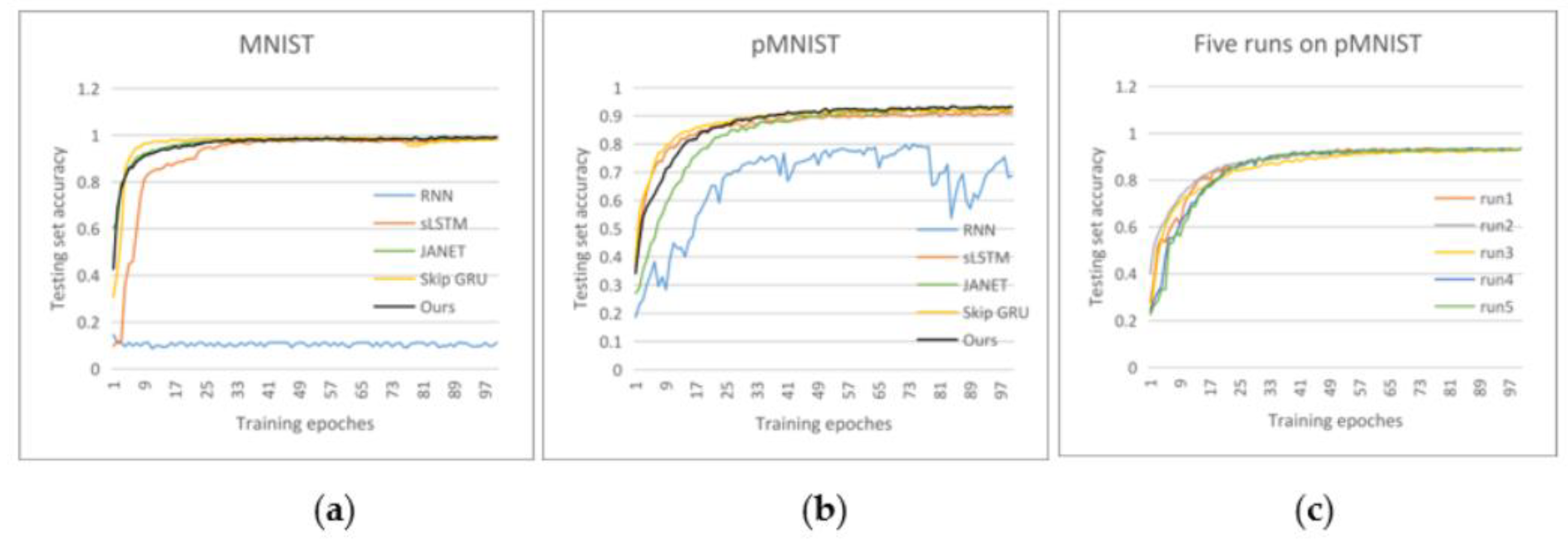
4.5. Classification Using MNIST and Permuted MNIST

In this section, we evaluate the methods considered on two publicly available datasets: the MNIST and the permuted MNIST (pMNIST) [17]. The MNIST comprises 55,000 images for training, 5000 for verification, and 10,000 for testing, where each of them is flattened from a size of 28 $\times$ 28 into 784-dimensional. The pMNIST is generated by permuting the image pixels in the MNIST and intends to create longer-term dependencies [17].

The means and standard deviations of the testing accuracy are presented in

Table 3. Results of the testing accuracy.

Model Dataset	Accuracy on MNIST	Accuracy on pMNIST
RNN	10.8 ± 0.689	67.8 ± 20.18
sLSTM	98.5 ± 0.183	91.0 ± 0.518
JANET	99.0 ± 0.120	92.5 ± 0.767
Skip GRU	98.9 ± 0.099	92.7 ± 0.738
Ours	99.1 ± 0.093	93.2 ± 0.483
iRNN [16]	97.0	82.0
uRNN [17]	95.1	91.4
TANH-RNN [16]	35.0	–
LSTM [15]	98.9	–
BN-LSTM [15]	99.0	–

, where the values are displayed in percentage form. We produced the results of our model and the results of Skip GRU on the datasets over five independent runs, and following the experimental setup in JANET [4], we utilized two hidden layers with 128 units for the MNIST and a single layer with the same units for the pMNIST. Then, as for the other results, we cited the presented results directly and the total number of layers or runs have been declared in their works; for instance, RNN, sLSTM, and JANET all utilized two layers on the MNIST and performed ten runs independently. From Table 3, we can see that our model achieved the best accuracy and had the most stable performance due to its minimum standard deviations.

The test accuracies on two datasets over the epochs of training are depicted in Figure 2a,b. We executed the programs of all the comparative methods and obtained the average results over five runs. Regarding the results using the MNIST set, which are presented in Figure 2a, all the methods behaved well, except for the RNN, and the Skip GRU converged the quickest in the beginning stage, whereas our method eventually achieved the best accuracy. Figure 2b depicts the accuracy curves for the methods used on pMNIST, which was more challenging than the MNIST; all the methods had a slower ascent to reaching their highest accuracies. Our method obtained the best accuracy compared with others, although its ascent curve was not the steepest. We also present the curves of different runs in Figure 2c, from which we can see that the curves differed from each other in the ascent stage but reached similar final maximum values. The sampled skip connections in our network partly contributed to this phenomenon as proper connections could accelerate the network’s convergence.

5. Conclusions

In this paper, we propose a neural network with random skip connections based on a neural architecture search scheme. A dense network is used for the construction of the search space, and then skip connections are generated via random sampling. To make the network computation efficient, we designed a novel cell structure that requires less memory and computational power; moreover, a special initialization scheme was utilized for parameter setting. In the experiments, we evaluated the models in four kinds of tasks. Several state-of-the-art methods were adopted for comparison and different criteria were used for evaluation. The experimental results demonstrated that our model behaved better than the other methods used for comparison in terms of different criteria. In the future, we plan to use reinforcement learning to search for the optimal architecture and compare the performance with our proposed method.

References

1. Dai, A.M.; Le, Q.V. Semi-supervised Sequence Learning. arXiv 2015, arXiv:1511.01432. [Google Scholar]
2. Hochreiter, S.; Schmidhuber, J. Long short-term memory. Neural Comput. 1997, 9, 1735–1780. [Google Scholar] [CrossRef]
3. Yao, K.; Cohn, T.; Vylomova, K.; Duh, K.; Dyer, C. Depth-gated recurrent neural networks. arXiv 2015, arXiv:1508.03790. [Google Scholar]
4. Westhuizen, J.V.D.; Lasenby, J. The unreasonable effectiveness of the forget gate. arXiv 2018, arXiv:1804.04849. [Google Scholar]
5. Campos Camunez, V.; Jou, B.; Giro-i-Nieto, X.; Torres, J.; Chang, S.F. Skip rnn: Learning to skip state updates in recurrent neural networks. In Proceedings of the Sixth International Conference on Learning Representations, Vancouver, BC, Canada, 30 April–3 May 2018; pp. 1–17. [Google Scholar]
6. Chang, S.; Zhang, Y.; Han, W.; Yu, M.; Guo, X.; Tan, W.; Cui, X.; Witbrock, M.; Hasegawa-Johnson, M.A.; Huang, T.S. Dilated recurrent neural networks. In Proceedings of the Advances in Neural Information Processing Systems, Long Beach, CA, USA, 4–9 December 2017; pp. 77–87. [Google Scholar]
7. Chung, J.; Ahn, S.; Bengio, Y. Hierarchical multiscale recurrent neural networks. arXiv 2016, arXiv:1609.01704. Available online: http://arxiv.org/abs/1609.01704 (accessed on 6 May 2016).
8. Elsken, T.; Hendrik Metzen, J.; Hutter, F. Neural architecture search: A survey. arXiv 2018, arXiv:1808.05377. [Google Scholar]
9. Bello, I.; Zoph, B.; Vasudevan, V.; Le, Q.V. Neural optimizer search with reinforcement learning. In Proceedings of the 34th International Conference on Machine Learning-Volume 70, Sydney, Australia, 6–11 August 2017. [Google Scholar]
10. Brock, A.; Lim, T.; Ritchie, J.M.; Weston, N. SMASH: One-shot model architecture search through hypernetworks. arXiv 2017, arXiv:1708.05344. Available online: http://arxiv.org/abs/1708.05344 (accessed on 17 August 2017).
11. Tallec, C.; Ollivier, Y. Can recurrent neural networks warp time? arXiv 2018, arXiv:1804.11188. [Google Scholar]
12. Neil, D.; Pfeiffer, M.; Liu, S.C. Phased lstm: Accelerating recurrent network training for long or event-based sequences. In Proceedings of the Advances in Neural Information Processing Systems, Barcelona, Spain, 5–10 December 2016; pp. 3882–3890. [Google Scholar]
13. El Hihi, S.; Bengio, Y. Hierarchical recurrent neural networks for long-term dependencies. In Proceedings of the Advances in Neural Information Processing Systems, Denver, CO, USA, 2–5 December 1996; pp. 493–499. [Google Scholar]
14. Zhang, S.; Wu, Y.; Che, T.; Lin, Z.; Memisevic, R.; Salakhutdinov, R.; Bengio, Y. Architectural complexity measures of recurrent neural networks. In Proceedings of the Advances in Neural Information Processing Systems, Barcelona, Spain, 5–10 December 2016; Available online: http://arxiv.org/abs/1602.08210 (accessed on 12 November 2016).
15. Lipton, Z.C.; Berkowitz, J.; Elkan, C. A critical review of recurrent neural networks for sequence learning. arXiv 2015, arXiv:1506.00019. [Google Scholar]
16. Le, Q.V.; Jaitly, N.; Hinton, G.E. A simple way to initialize recurrent networks of rectified linear units. arXiv 2015, arXiv:1504.00941. Available online: http://arxiv.org/abs/1504.00941 (accessed on 7 April 2015).
17. Arjovsky, M.; Shah, A.; Bengio, Y. Unitary evolution recurrent neural networks. In Proceedings of the 33rd International Conference on Machine Learning (ICML 2016), New York, NY, USA, 19–24 June 2016; pp. 1120–1128. Available online: http://jmlr.org/proceedings/papers/v48/arjovsky16.html (accessed on 25 May 2016).
18. Kingma, D.P.; Ba, J. Adam: A method for stochastic optimization. arXiv 2014, arXiv:1412.6980. Available online: http://arxiv.org/abs/1412.6980 (accessed on 22 December 2014).
19. Razvan Pascanu, T.M.; Bengio, Y. On the difficulty of training recurrent neural networks. In Proceedings of the International Conference on Machine Learning, Atlanta, GA, USA, 16–21 June 2013; pp. 2342–2350. [Google Scholar]
20. Adolf, R.; Rama, S.; Reagen, B.; Wei, G.; Brooks, D.M. Fathom: Reference work-loads for modern deep learning methods. In Proceedings of the 2016 IEEE International Symposium on Workload Characterization (IISWC), Providence, RI, USA, 25–27 September 2016; Available online: http://arxiv.org/abs/1608.06581 (accessed on 23 September 2016).
Figure 1. The framework of our proposed model. RNN: Recurrent neural network.
Applsci 10 03712 g001
Figure 2. The change in test accuracy with training epochs. (a) accuracy on the MNIST, (b) accuracy on the pMNIST, (c) accuracy over five runs on the pMNIST.
Applsci 10 03712 g002