CARMA—Cellular Automata with Refined Mesh Adaptation—The Easy Way of Generation of Structural Topologies

Abstract

This paper is focused on the development of a Cellular Automata algorithm with the refined mesh adaptation technique and the implementation of this algorithm in topology optimization problems. Traditionally, a Cellular Automaton is created based on regular discretization of the design domain into a lattice of cells, the states of which are updated by applying simple local rules. It is expected that during the topology optimization process the local rules responsible for the evaluation of cell states can drive the solution to solid/void resulting structures. In the proposed approach, the finite elements are equivalent to cells of an automaton and the states of cells are represented by design variables. While optimizing engineering structural elements, the important issue is to obtain well-defined solutions: in particular, topologies with smooth boundaries. The quality of the structural topology boundaries depends on the resolution level of mesh discretization: the greater the number of elements in the mesh, the better the representation of the optimized structure. However, the use of fine meshes implies a high computational cost. We propose, therefore, an adaptive way to refine the mesh. This allowed us to reduce the number of design variables without losing the accuracy of results and without an excessive increase in the number of elements caused by use of a fine mesh for a whole structure. In particular, it is not necessary to cover void regions with a very fine mesh. The implementation of a fine grid is expected mainly in the so-called grey regions where it has to be decided whether a cell becomes solid or void. The benefit of the proposed approach, besides the possibility of obtaining high-resolution, sharply resolved fine optimal topologies with a relatively low computational cost, is also that the checkerboard effect, mesh dependency, and the so-called grey areas can be eliminated without using any additional filtering. Moreover, the algorithm presented is versatile, which allows its easy combination with any structural analysis solver built on the finite element method.

1. Introduction

Topology optimization is still one of the most important issues in the field of optimal design of engineering structures. It has gained enormous popularity, for many years being an effective tool applied to innovative design projects with a wide range of applications in various areas, including mechanical engineering, civil engineering, bioengineering, material science, and many others. Today, the interest of researchers and designers is mainly focused on improving the quality, versatility, and effectiveness of optimization algorithms to be applied to solving demanding engineering design tasks. Apart from studies on theoretical issues, e.g., [1,2], new numerical algorithms and methods, e.g., [3], and innovative applications, the attention is focused on computational efficiency and accuracy. Modern fast algorithms are developed with the aim of getting optimization codes, which will guarantee that a relatively small number of iterations is needed. At the same time, the reduction of the dimensionality of problems, combined with the refined mesh adaptation, has been considered. Since the first implementation of adaptive mesh in topology optimization [4], the concept of reduction of the number of design variables has become popular, because it allows creation of similar topologies, compared to those with a large number of design variables involved, without extensive computational effort. Moreover, mesh refinement allows inexpensive but efficient improvement of the finite element solution, as shown in [5,6]. A broad discussion of the current state of knowledge can be found in [7,8,9]. Most published papers focused on adaptive strategies discuss filtering, e.g., [10], errors indicators [11,12], or some aspects of a finite element grid, e.g., [13,14].

This paper is focused on the development of a Cellular Automata algorithm with the refined mesh adaptation technique, and the implementation of this algorithm in topology optimization problems. The versatility of the method was confirmed by the results of numerical tests performed for structures under one- and two-load cases, and also for the design-dependent self-weight loading. The results were compared with solutions gained for very fine mesh to confirm their correctness. In this paper, the discussion is also expanded to include some results obtained using algorithms proposed by other authors.

2. The Aim of the Paper

While optimizing engineering structural elements, the important issue is to obtain well-defined solutions, in particular, topologies with smooth boundaries. The quality of the structure topology boundaries depends mainly on the resolution level of mesh discretization; usually the greater the number of elements in the mesh, the better the representation of the optimized structure (see Figure 1).

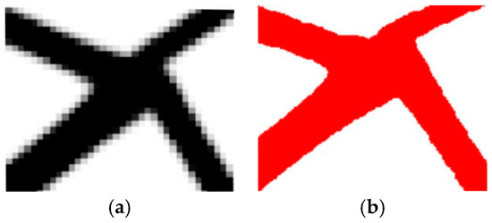
Figure 1. Mesh refining as the remedy for non-smooth boundaries: (a) example of a coarse mesh; (b) example of a fine mesh.

One can observe, however, that even for a very dense mesh, the so-called grey elements can still be present at the boundaries, even if some filtering techniques have been implemented (see Figure 2). This is because these techniques mainly reduce the effect of mesh dependency and not necessarily eliminate grey elements. This usually requires additional filtering.

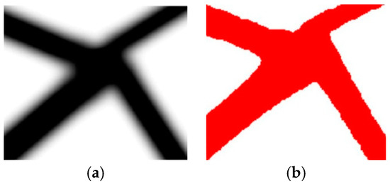
Figure 2. Mesh refining may not eliminate grey elements: (a) example of a fine mesh with the presence of grey elements; (b) example of a fine mesh without grey elements at boundaries.

It can be observed that while implementing dense meshes some thin and slender parts of structural topology can appear. This effect should also be controlled by filtering techniques (see Figure 3).

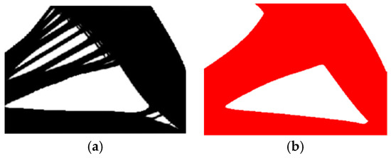
Figure 3. The appearance of thin and slender parts of structural topology in the case of a fine mesh has to be controlled by filtering techniques: (a) example of a fine mesh without filtering; (b) example of a fine mesh with filtering.

All of the abovementioned issues have to be taken into consideration while developing topology generators for engineering applications. The main goal is to achieve a regular, well-defined structural layout. It seems that the remedy for the above can be the implementation of refined mesh adaptation techniques. Adaptive mesh refinement allows for reduction of the number of design variables without losing the accuracy of results and without an excessive increase in the number of elements caused by using a fine mesh for the whole structure. It is possible to obtain high-resolution optimal topologies with a relatively low computational cost. It is not necessary to cover void regions or solid regions, the appearance and necessity of which are detected in the very first stage of optimization process with a very fine mesh. The implementation of a fine grid is expected to be used mainly for the so-called grey regions, where it is decided whether a cell becomes solid or void. The benefit of such an approach is also that the checkerboard effect and the so-called grey areas can be eliminated without using any additional filtering.

The aim of this paper is to develop a Cellular Automata algorithm with the refined mesh adaptation technique and to present the implementation of this algorithm into topology optimization problems.

3. Topology Optimization Using the Cellular Automata Method

The concept of topology optimization can be dated back to 1904 and is attributed to the paper by Michell [15], but the papers by Bendsoe and Kikuchi [16], and Bendsoe [17] published in the late 1990s sparked the development of this research area. The idea of topology optimization is to find a material layout which meets the assumed criteria, and in this sense gives the optimal solution. During the optimization process, the material is redistributed within the desired design domain, which leads to the creation of a new shape of optimized structure.

In topology optimization, the computational design domain is discretized and represented by finite elements, for which design variables called relative densities $d_i$ are selected. The material representation can be defined using the well-known and broadly accepted solid isotropic material with penalization (SIMP) approach, e.g., [18,19], where the elastic modulus $E_i$ of each element is a function of relative density $d_i$:

$$E_i=d_i^p{E}_0, d_{min}\le d_i\le 1.$$

(1)

In Equation (1), $E_0$ is the Young modulus of a solid material, whereas the power $p$(usually equal to 3) is introduced to penalize intermediate densities. The constraints are imposed on the design variables, and $d_{min}$ in Equation (1) is a non-zero minimum relative density introduced in order to avoid singularity.

For the design domain discretized and represented by finite elements, the topology optimization problem aimed at minimizing the function of compliance $U\left(d\right)$of a structure subject to a total volume constraint can be expressed as (see Equation (2)):

$$\begin{array}{c}\hfill \mathrm{minimize}\\ \hfill \mathrm{subject} \mathrm{to}\end{array}\begin{array}{cc}& \hspace{1em}\hspace{1em}\hspace{1em}U\left(d\right)=u^{T}ku={\displaystyle {\displaystyle \sum }_{i=1}^N}{d}_i^p{u}_i^T{k}_i{u}_i\\ & V\left(d\right)=\kappa V_0\\ \hspace{1em}\hspace{1em}\hspace{1em}\hspace{1em}ku=f& \end{array}$$

(2)

In (2), $u$ and $f$ are the global displacement and force vectors, $k$ is the global stiffness matrix, $u_i$ and $k_i$ are the element displacement vector and stiffness matrix, respectively, and $N$ is the number of elements. Simultaneously, a constraint imposed on global volume of a structure, represented by the function $V\left(d\right)$ of the design variables $d_i$, has been applied for a specified volume fraction $\kappa$, and $V_0$ standing for the initial design domain volume. A broad discussion of the principles of topology optimization can be found, for example, in [16,17,18,20].

Simultaneously with the development of the topology optimization area, especially within engineering applications, numerous numerical optimization techniques aimed at solving newly formulated problems efficiently and quickly have been proposed. Some of those optimization techniques are based on gradient information, e.g., the optimality criteria method [21,22] or level set methods [21,22,23], some others implement non-gradient evolutionary techniques [23]. Among many proposals one can also find Cellular Automata (CA). This method has become more and more popular since the introduction of the concept by von Neumann [24] and Ulam [25]. However, the application of Cellular Automata to structural optimization has occurred only in the last two decades. In particular, this concept has been successfully applied to topology optimization, which was illustrated in a series of published papers, e.g., [26,27,28,29,30,31]. In particular, the efficiency of the Cellular Automata method is discussed in [32].

The idea of Cellular Automata is to model a complex system by its discrete idealization and to mimic system performance based on local interactions governed by simple local update rules. The application of CA requires decomposition of the design domain into a lattice of cells, which can have influence only on the neighboring cells. The examples of plane neighborhoods for rectangular cells are presented in Figure 4.

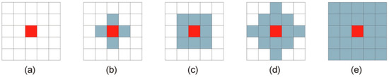
Figure 4. Neighborhoods for plane problems: (a) empty; (b) von Neumann; (c) Moore; (d) MvonN; (e) extended Moore.

Having selected a neighborhood, the problem can now be formulated as a set of local minimizations posed for each element:

$$\min U\left(d_i\right)=d_i^p{u}_i^T{k}_i{u}_i$$

(3)

In order to solve the problem, a heuristic, local CA update rule is here proposed, utilizing the information gathered from a selected neighborhood. New values of design variables can be calculated based on the Gauss-Seidel iteration mode, i.e., cell updates its state based on updated values found for cell neighbors in the current and previous iteration, or on the Jacobi iteration mode, i.e., cell updates its state based on the states of the surrounding cells obtained in the previous iteration only. This scheme was chosen for this paper. In what follows:

$$d_i^{\left(t+1\right)}=d_i^{\left(t\right)}+\mathsf{∆}{d}_i^{\left(t\right)},$$

(4)

where t is the current iteration and:

$$\mathsf{∆}{d}_i^{\left(t\right)}=\frac{1}{M+1}\left({\alpha }_i+{\displaystyle \sum }_{k=1}^M{\alpha }_{ik}\right)m .$$

(5)

The rule is illustrated in Figure 5:

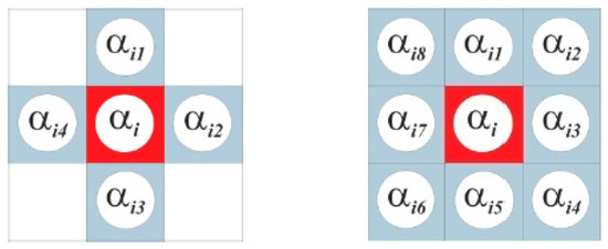
Figure 5. Updating the density of a central cell is based on information gathered among neighboring rectangular cells. The von Neumann (left) and Moore (right) neighborhood.

In Equation (5) $m$ denotes move limit (e.g., $m$ = 0.2), coefficients, ${\alpha }_i$ (for central cell $i$) and ${\alpha }_{ik}$ (for M neighboring cells) are calculated based on the concept preliminary reported in [33]—see Equation (6):

$${\alpha }_i=\{\begin{array}{c}-C_{\alpha } \mathrm{if} U_i<U_1\\ f\left(U_i\right) \mathrm{if} U_1 \le U_i\le U_2\\ C_{\alpha } \mathrm{if} U_i>U_2 ,\end{array} {\alpha }_{ik}=\{\begin{array}{c}-C_{\alpha } \mathrm{if} U_{ik}<U_1\\ f\left(U_{ik}\right) \mathrm{if} U_1 \le U_{ik}\le U_2\\ C_{\alpha } \mathrm{if} U_{ik}>U_2 ,\end{array}$$

(6)

where $U_i , U_{ik}$ are the values of compliances of the central and neighboring cells, $U_1$ and $U_2$ are the threshold values of compliances which separate cells of the lowest and the largest compliances, and can be selected for each example. For the remaining cells, the linear function was built to fulfill the assumptions $f\left(U_1\right)=-C_{\alpha }$ and $f\left(U_2\right)=C_{\alpha }$

$$f\left(U\right)=\frac{2C_{\alpha }}{U_2-U_1}U-C_{\alpha }\frac{U_2+U_1}{U_2-U_1} .$$

(7)

4. Numerical Treatment

The numerical algorithm has been built in order to apply the above proposed approach to the generation of structural topologies.

4.1. General

As to the iterative optimization procedure, the sequential/nested approach has been adapted. Thus, for each iteration a structural analysis for the optimized element is performed first, and then the local updating rules are applied. It means that the objective is computed from the state solution obtained, and the design field is updated based on the local rule. As for the material density, the design variables field follows the discretization of the FEM solver.

One of the assumptions was to combine the algorithm with a professional structural analysis code. The CA topology generator introduced can easily be combined with such programs. In this paper, the finite element analysis tool ANSYS stands for the structural analysis module.

The global volume constraint can be applied for a specified volume fraction. The volume constraint is implemented in each iteration when local update rules have been applied to all elements. In practice, the design variables multiplier is introduced, and then its value is sought, to fulfill the volume constraint. As a result, the topologies generated preserve a specified volume fraction of a solid material during the optimization process.

In the present study, the assumed change of the objective function value for subsequent iterations was implemented as the stopping criterion, but in general it can also be defined as performing a selected number of iterations.

4.2. The Local Rule

As for the practical numerical realization of the CA local rule (4)–(7), it is proposed to introduce the threshold number of cells, instead of the threshold compliance value. To do this, the cell compliances are sorted in ascending order and consecutive indices $n$ are ascribed to the sorted cells. In what follows, $U_1$ and $U_2$ can be replaced now by $N_1$ and $N_2$, where $N_1$ is the number of elements of the smallest compliance and $N-N_2$ stands for the number of elements of the largest compliance. Equation (7) can be rewritten in the form of Equation (8):

$$f\left(n\right)=\frac{2C_{\alpha }}{N_2-N_1}n-C_{\alpha }\frac{N_2+N_1}{N_2-N_1}$$

(8)

In this method, $C_{\alpha }=1$ is implemented, but a selection is not restricted to this value. It is important to underline that in the presented algorithm, only two parameters to adjust are defined, namely $N_1$ and $N_2$. One can select these values to control and tune the algorithm performance, for example, start with a wide interval $\left[N_1{N}_2\right],$ decreasing it as the generation of topologies proceeds. Based on numerical tests performed, it is recommended to start with the selection: $N_1=0.1 N$ and $N_2=0.9 N$, which means the selection of 10 percent of elements in both the subset of the smallest and the subset of the largest compliances. After a given number of iterations, the values of $N_1$ and $N_2$ can be modified. For the test examples in this paper, after 20 iterations the value $N_1=0.7 N$, whereas $N_2=0.9 N$remained unchanged. It has been observed that adjusting the interval $\left[N_1{N}_2\right]$ can speed up the process of eliminating the so-called grey elements at the final stage of topology generation.

4.3. Neighborhood

Each cell has the same selected neighborhood, therefore those at the boundary have neighboring cells that lie outside the design domain. For those cells, the values of the design variables must be also specified. The most common approach, utilized in this paper, is to set all these values to a fixed value; zero is the usual choice. As an alternative, adiabatic or reflecting boundary conditions (e.g., [29]) can also be adopted (see Figure 6).

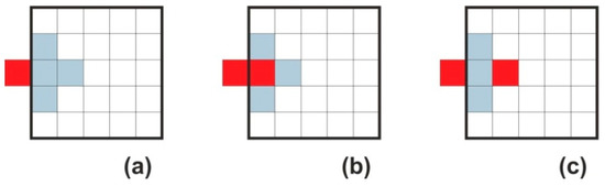
Figure 6. Boundary cells: (a) fixed; (b) adiabatic; (c) reflected.

4.4. The Pseudo-Code

Below, in Table 1, the pseudo-code of the proposed algorithm is listed.

Table 1. The pseudo-code of the proposed algorithm.

GET input data SELECT initial mesh—material density field follows FEM discretization SET initial values of design variables SELECT neighborhood type ASSIGN neighbors to each element SELECT values of control parameters $N_1$ and $N_2$ SELECT move limit $m$ DO UNTIL stopping criteria are met INTRODUCE mesh adaptation if required PERFORM structural analysis—ANSYS solver   IMPORT data from structural analysis    FOR all elements      CALCULATE local compliances $U_i$    END FOR   CALCULATE ${\alpha }_i$ and ${\alpha }_{ik}$    FOR all elements      UPDATE design variables $d_i$     END FOR   IMPOSE volume constraint END DO

5. Cellular Automata Algorithm with Refined Mesh Adaptation

The effectiveness of any algorithm applied to solve topology optimization problems relies on the computational effort required to obtain the optimal solution in terms of the number of iterations to perform, number of elements used in the structural analysis, number of design variables, and so on. This computational effort can be reduced by introducing a non-regular mesh of finite elements during the iteration process, by adapting the algorithm to perform mesh refinement within selected regions of the design domain. From the numerical point of view, it is not so obvious where and how to apply such refining, and it is generally assumed that this choice is related to the problem under consideration [34]. For example, the regions of stress concentration or the value of the numerical error indicator can suggest the refinement. While performing topology optimization, the attention is focused on the regions where it has to be decided whether design elements become solids or voids, i.e., on the so-called grey regions defined by the refinement indicator γ_i [10]:

$${\gamma }_i=\left(1-d_i\right)d_i.$$

(9)

According to [10], the value of γ_i ≥ 0.16 indicates the necessity of refinement of the ith element. Nevertheless, the numerical studies performed have shown that this value can be slightly modified and adjusted to specific examples being considered. It is also possible to choose a different adaptive strategy based on, for example, the values of compliance or stress calculated for design cells. Based on preliminary studies, one can state that the adjustments of the boundary values of the refinement indicator have a more significant influence on the final refinement than the values of physical quantities on which they are defined. It is also worth mentioning that the function in Equation (9) does not need to be a quadratic function, including asymmetry. This issue could be investigated in detail in further research.

Based on the above discussion, the mesh refinement was applied to inner and outer boundaries to improve the quality of the boundary representation. Importantly, it allows grey elements on the boundaries to be avoided, and a solid/void (black-and-white) structure to be obtain, at the same time controlling the mesh resolution. The proposed Cellular Automata approach does not require any additional density filtering to generate solid/void topologies, and the simplest refinement strategy described above is entirely sufficient to meet a condition of smooth boundaries with a very fine mesh.

To control the process of the mesh refinement, the principles described, e.g., in [6] and [8] were adopted. The first rule is to keep the element size within the defined range, i.e., the smallest size of elements which can be refined is set. That prevents the creation of very small elements, which bring no improvement to the solution. The next issue is when to apply a refinement. If it is applied too early, after a small number of iterations, a large number of cells will be refined because of a large number of grey elements at this stage. In the end, this causes the profit from the reduction of the total elements number to be low. If refining is applied too late, the resulting topology can be formed by a coarse mesh, and the topology details may be omitted. Detailed discussion of this issue can be found in [7].

The main goal of the work described in this paper was the reduction of the number of finite elements in mesh discretization during topology optimization, without losing the accuracy of the final solution. Various strategies of mesh refinement were investigated, and based on that research, the authors propose a strategy which performed effectively when incorporated into the topology optimization algorithm. The idea employed in this paper is as follows. First, a given number (up to 10) of optimization steps are performed—those iterations are performed for a coarse mesh. At this stage, first void and solid elements appear, but the structure topology is still far away from the final solution. Based on the coarse mesh layout, the elements for the first refinement are selected. Hence, the second stage of the optimization process (i.e., up to 5 iterations), followed by the second refinement for the selected elements, is performed. The iterative procedure continues until the minimal allowable element size has been reached. This strategy eliminates the situation, when the refinement is applied too early, after a small number of iterations, and a large number of cells is refined because of a large number of grey elements at this stage. Fine mesh applied to the whole structure at an early stage of the process practically eliminates all advantages related to the adaptive strategy implementation, in particular the reduction of the number of elements. On the other hand, if refining is applied too late, the resulting topology can be formed by a coarse mesh and the topology details may be omitted. The number of iterations required for subsequent refinement stages is controlled by the user and may differ depending on the problem being solved.

As mentioned earlier, in this method the efficient finite element analysis tool ANSYS is used as the structural analysis module. The solution using the ANSYS package has more advantages, namely the refinement is carried out automatically after the optimization program has indicated refinement regions, and there are also various tools which can be used to improve element quality automatically at each step of the refining process. Additionally, the user can define any complicated geometry, or use different types of elements without implementing significant changes into the main optimization program.

The automatic mesh refinement of selected elements proceeds in order to get the resulting element edge length equal to approximately 0.5 of the original element edge length. The mesh created is free from so-called hanging nodes, because the neighboring cells of the refined element are affected (split) in order to preserve the transition between elements. In the automatic refinement of the meshing procedure, the depth of refinement is equal to one element outward of the selected cell, and introducing triangular elements is forbidden; these options can be defined in ANSYS. An illustration of the mesh refinement concept is presented in detail in Figure 7.

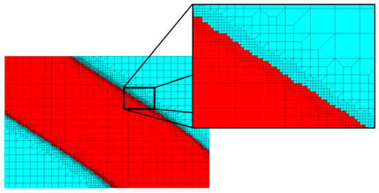
Figure 7. Mesh refining on the boundaries of the structure.

It is worth noting that within the regions of refinement, the number of neighboring cells can vary depending on the type of neighborhood.

6. Introductory Examples

6.1. The Square Cantilever Structure

As an introductory example of the implementation of the proposed idea, a plain elastic square structure, fixed along the left edge and loaded as presented in Figure 8, was chosen. The Young modulus and the Poisson ratio were E = 2 × 10¹¹ Pa and ν = 0.3, respectively. A volume fraction equal to 0.5 was implemented. A concentrated force P equal to 1000 N was applied.

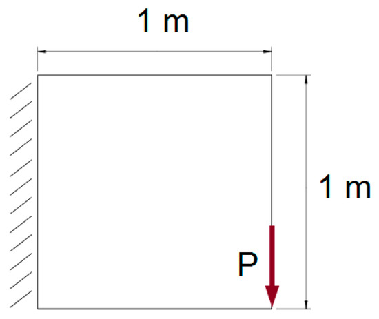
Figure 8. Initial structure with applied loads and supports, example 1.

First, the structure was discretized with a regular mesh of 2500 cells (0.0004 m²). The topology optimization with an adaptive refinement procedure was applied and the results are presented in Figure 9, where the selected middle topologies and the final one are shown. At the end of the optimization process, the resulting number of cells equaled 26,217. The final value of the compliance equaled 2.149·10⁻⁴ Nm. The iteration history showing the fast convergence to the final solution is provided in Figure 10.

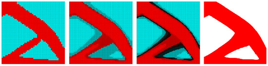
Figure 9. Selected middle topologies and the final one for the introductory example—for the last iteration, the grid has not been shown, to improve the clarity of the picture.

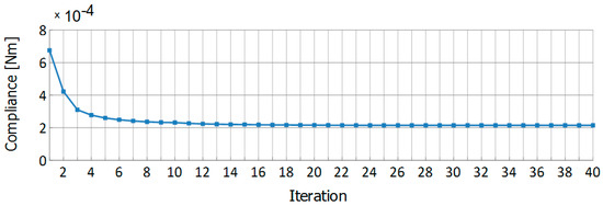
Figure 10. Iteration history for the introductory example.

For these calculations, the von Neumann neighborhood was chosen, but the implementation of the Moore one was also tested. According to the results of this study, the choice of the neighborhood type had no significant influence on the final results of the topology optimization for the examples discussed in this paper. Below (Figure 11), the final topologies found for von Neumann (left) and Moore (right) neighborhoods are presented. The final values of the compliance for both types were the same, i.e., 2.149·10⁻⁴ Nm.

Figure 11. The final topologies obtained for von Neumann (left) and Moore (right) neighborhoods.

To compare the results of the application of the Cellular Automata to the refined mesh adaptation with the results obtained for a regular mesh, the structure was discretized with a regular lattice of 211,600 elements (~4.726·10⁻⁶ m², see Figure 12d), which corresponds to the size of the smallest elements of the mesh formed during refinement. To get the results for the refined mesh and for the regular mesh, the proposed algorithm needed 39 and 48 iterations, respectively.

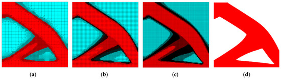
Figure 12. Final topologies obtained for four sizes of initial elements: 0.0025 m² (a), 0.0004 m² (b), 0.0001 m² (c) and ~4.726 × 10⁻⁶ m² regular mesh (d). For the last case the grid has not been shown to improve the clarity of the picture.

The comparison of the computing time for the example discussed was performed to illustrate the effectiveness of the proposed approach. The timing information for the case of mesh refinement, and calculation for the corresponding fine mesh, were taken into account. A clock-time was used as a metric of algorithm runtime. The calculation process consists of two main stages: FEM analysis and design variable update. For the optimization involving the mesh refinement, after a given number of iterations with initial mesh, two refinement processes were performed. The times of those processes had minimal influence on the final time of all calculations, and the profit from applying the mesh adaptation was not reduced by the need to carry out the mesh refinement. The time spent on an optimization iteration is less than 2 s, even for a large number of elements. The time consumption is therefore caused by the structural analyses. For the example considered (where a 4-node finite element was used), the total time of the whole process in the case of a mesh adaptation was equal to about 24 min, while for a fine uniform mesh it was more than 140 min. The ANSYS Mechanical 14.0 was used as the analysis tool with two Intel(R) Xeon(R) CPU E5645 2.4 GHz processors and 192 GB of RAM (64 bit architecture). It is important to underline that for every iteration for a regular mesh, 168 s are needed to perform the analysis, while for each step of a mesh refinement, 8, 15, and 45 s are needed, respectively.

To check if the resulting designs depend on the initial resolution of the mesh, the calculations were repeated for three sizes of initial elements: 0.0025 m², 0.0004 m², and 0.0001 m². Final topologies are presented in Figure 12, including those calculated for a regular mesh for 211,600 elements. In each case, the same number (2) of mesh refinements was performed during the adaptation process, to get a more appropriate comparison.

For the sake of comparison, this example was solved using both the code based on [35] with different filtering techniques, including the one based on Helmholtz type differential equations [36], and the code based on [37]. The results are given in Figure 13 and Figure 14, respectively.

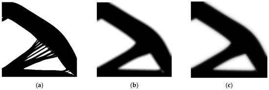
Figure 13. Final topology obtained using [35] with a small (a) and a large filtering radius. Case (b) refers to density filtering, whereas case (c) is the result of application of filtering based on Helmholtz-type differential equations.

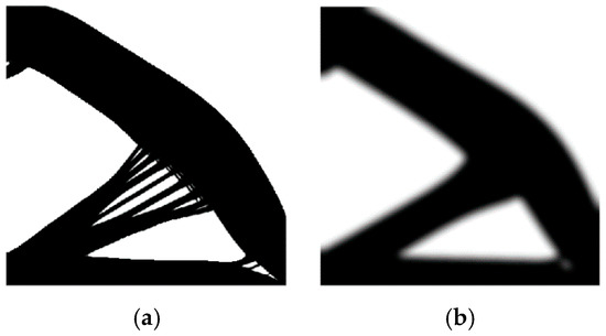
Figure 14. Final topology obtained using [37] with a small (a) and a large (b) filtering radius.

Additionally, the initial irregularities in the mesh were introduced to illustrate the flexibility of the method. Irregularities (a denser mesh) were located in places with the expected concentration of stresses for the initial structure (see Figure 15). The final value of the compliance equaled 2.388 × 10⁻⁴ Nm. The iteration history is shown in Figure 16.

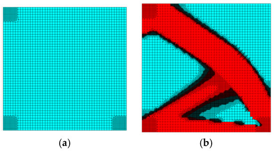
Figure 15. Initial irregularity of the mesh density (a) and the final topology (b).

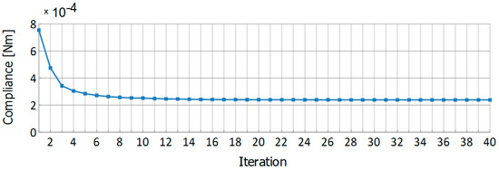
Figure 16. Iteration history for the introductory example for the mesh presented in Figure 15.

6.2. The Rectangular Cantilever Structure

As a second introductory example, a plain elastic structure fixed along the left edge, and loaded with three concentrated forces, as presented in Figure 17, was chosen. The Young modulus and the Poisson ratio were E = 2 × 10¹¹ Pa and ν = 0.3, respectively, and P equaled 1000 N. A volume fraction equal to 0.5 was implemented.

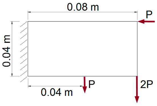
Figure 17. Initial structure with applied loads and supports, example 2.

In the first step, the structure was discretized with a regular mesh of 1500 cells. The topology optimization with a refining procedure was applied, and the results, including selected iterations and final topology, and the iteration history, are presented in Figure 18 and Figure 19, respectively. At the end of the optimization process, the resulting number of cells equaled 33,853, and the final value of the compliance equaled 0.820·10⁻⁵ Nm. To cover the whole structure with a fine mesh with 8-node elements (the same size as the smallest elements as in the refined grid), 101,250 elements were needed. For the example considered, the total time of the whole process in the case of a mesh adaptation was equal to about 37 min, while for a fine uniform mesh it was more than 250 min. It is important to underline that for every iteration for a regular mesh, 500 s are needed to make an analysis, while for each step of a mesh refinement, 7, 33, and 85 s are needed, respectively. The computational cost is generated mostly by the structural analysis. Time spent on updating the design variables is 1–2 s per iteration, the optimization part returns an almost immediate response.

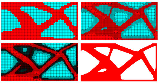
Figure 18. Selected middle topologies and the final one for the cantilever structure. For the last iteration the grid has not been shown to improve the clarity of the picture.

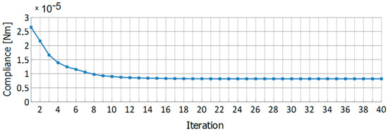
Figure 19. The iteration history for the cantilever structure.

For comparison, this example was calculated using both the code based on [35] and the code based on [37]. The results are given in Figure 20 and Figure 21, respectively.

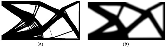
Figure 20. The final topology obtained using [35] with a small (a) and a large (b) filtering radius.

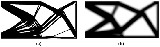
Figure 21. The final topology obtained using [37] with a small (a) and a large (b) filtering radius.

7. The Algorithm Performance

7.1. The T-bracket Structure

To examine the proposed Cellular Automata method combined with the refined mesh adaptation, more complicated geometries were investigated. The first of them is a T-bracket structure (see Figure 22).

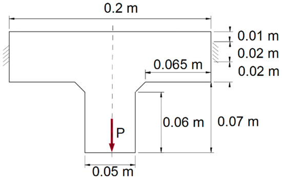
Figure 22. The T-bracket example, an initial structure with applied loads and supports.

Half of the element was considered due to symmetry. The Young modulus and the Poisson ratio were E = 2 × 10¹¹ Pa and ν = 0.3, respectively. A volume fraction equal to 0.5 was implemented, a concentrated force P = 1000 N was applied. As in the previous example, the dynamic mesh refinement was implemented for an initially regular mesh of 775 elements. The initial mesh, a selected iteration, and the final topology for this example are shown in Figure 23. The compliance value of the optimized structure equals 1.741·10⁻⁴ Nm, the iteration history is presented in Figure 24.

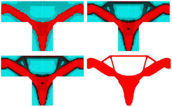
Figure 23. Selected middle topologies and the final one for the T-bracket structure—for the last iteration the grid has not been shown to improve the clarity of the picture.

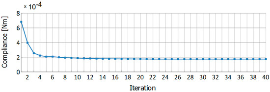
Figure 24. The iteration history for the T-bracket example.

At the end of the optimization process, the number of elements equaled 16,472, while the regular mesh needed 130,896 elements to cover the whole structure with elements of the same size as the smallest cell of irregular mesh.

To illustrate the results obtained for a regular mesh, the final topologies for 1830, 7180, 15,359, and 130,896 elements are presented in Figure 25.

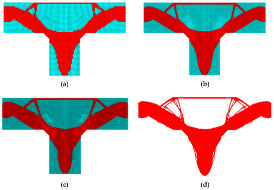
Figure 25. The final topologies for 1830 (a), 7180 (b), 15,359 (c), and 130,896 (d) elements. In the last case a grid has not been shown to improve the clarity of the figure.

For comparison, this example was calculated using the code based on [35]. The resulting topology is given in Figure 26.

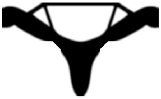
Figure 26. The final topology obtained using [35].

7.2. The Kneestructure

A knee-structure was chosen as the next example to illustrate the performance of a proposed methodology (Figure 27). The Young modulus and the Poisson ratio were E = 2 × 10¹¹ Pa and ν = 0.3, respectively. A volume fraction equal to 0.5 was implemented, and force P = 1000 N.

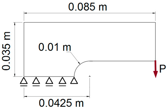
Figure 27. The knee structure, an initial structure with applied loads and supports.

The optimization process started with 645 elements, and at the end the mesh consisted of 18,191 elements. To cover the whole structure with the same very fine mesh, 69,348 elements were required. The final value of a compliance equaled 1.486·10⁻⁴ Nm. Selected middle topologies and the final one are presented in Figure 28, the iteration history is presented in Figure 29.

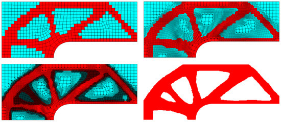
Figure 28. Selected middle topologies and the final one for the knee structure. For the last iteration the grid has not been shown to improve the clarity of the picture.

Figure 29. Iteration history for the knee structure.

Next, this example was calculated with the code based on [35], with the resulting topology shown in Figure 30.

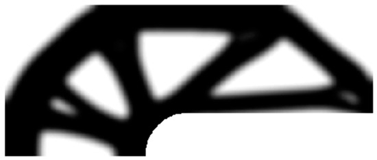
Figure 30. The final topology obtained using [35].

7.3. The Plane Structure with Holes

The plane symmetric structure with holes presented in Figure 31 was selected to illustrate the performance of the algorithm for more complicated geometry. The radii of the holes were R1 = 0.075 m, R2 = 0.03 m, R3 = 0.045 m. The Young modulus and the Poisson ratio were E = 2 × 10¹¹ Pa and ν = 0.3, respectively. A volume fraction equal to 0.75 and a concentrated force P = 1000 N were applied.

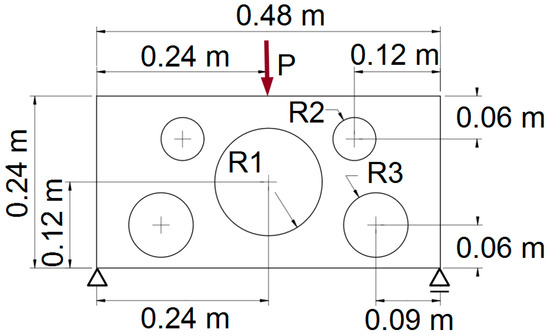
Figure 31. The initial structure with applied loads and supports.

The optimization process started with 2818 and at the end the mesh consisted of 34,596 elements. To cover the whole structure with the same very fine mesh, 770,775 elements were required. The final results are presented in Figure 32 and the iteration history is presented in Figure 33. The final value of the compliance equaled 0.716·10⁻³ Nm.

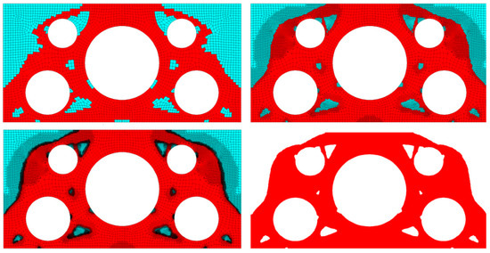
Figure 32. Selected middle topologies and the final one for the plane structure with holes. For the last iteration the grid has not been shown to improve the clarity of the picture.

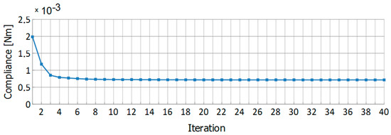
Figure 33. Iteration history for the plane structure with holes.

In this case of a mesh with high irregularities, an additional CA rule was introduced; solid elements that are surrounded by voids are converted into voids, and vice versa. This prevents the appearance of sharp details along the edges.

The example was calculated with the code based on [35] with resulting topology shown in Figure 34.

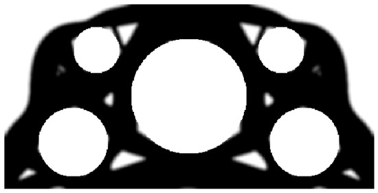
Figure 34. The final topology obtained using [35].

7.4. Topology Optimization for a Multiple Load Case

As the example of the two-load scheme, a plain elastic square structure fixed along the left edge and loaded as shown in Figure 35 was chosen. The Young modulus and the Poisson ratio were E = 2 × 10¹¹ Pa and ν = 0.3, respectively. A volume fraction equal to 0.4 was implemented, and a concentrated force P = 4000 N was applied.

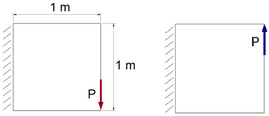
Figure 35. The initial structure with applied loads—the two loads scheme and support.

The initial regular mesh consisted of 1156 elements. The topology optimization steps (selected iterations) with mesh refinement are presented in Figure 36. The iteration history is shown in Figure 37. The final value of the compliance equaled 0.451 × 10⁻² Nm.

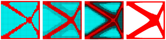
Figure 36. Selected middle topologies and the final one for the structure under two-load case—for the last iteration the grid has not been shown, to improve the clarity of the picture.

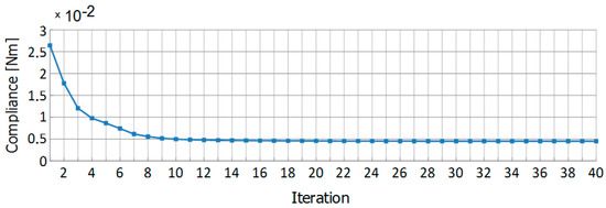
Figure 37. Iteration history for the structure under two-load case.

At the end of the optimization process according to the refinement, the resulting number of cells equaled 44,034, while the regular mesh needed 92,416 elements to cover the whole structure with elements of the same size as the smallest cell of the irregular mesh. The resulting topology was free from grey elements on the boundaries, small holes, and thin elements, which is desirable from the point of view of the manufacturing technology. This effect was gained without additive filtering, in contrast to the studies presented in [38].

7.5. Topology Optimization under Self-Weight Load

Including design-dependent loading like self-weight makes the examples considered more practical and realistic, but computationally more demanding. On the other hand, this aspect has significant importance while considering, for example, massive engineering structures. The problem of topology optimization with design-dependent loads is discussed, for example, in [39] and [40]. When dealing with self-weight loading, the modification and extension of a standard SIMP method is necessary (see [41]), so that the material density ρ_i of each element is defined according to Equation (8):

$${\rho }_i=d_i^p{\rho }_0.$$

(10)

It is worth noticing that the total volume constraint can be inactive while considering topology optimization, including self-weight loading. The right choice of algorithm control parameters can prevent this problem.

A rectangle (2 m × 1 m) supported at the left and right lower corners under self-weight was investigated to illustrate the topology optimization under the presence of self-weight loading. Half of the element was considered due to the symmetry. The Young modulus E = 2 × 10¹¹ Pa and the Poisson ratio ν = 0.3, were implemented. The density of the material equaled ρ = 8000 kg/m³. The volume fraction was equal to 0.5. Only self-weight loading was taken into account. The initial regular mesh consisted of 400 elements, and at the end of the refinement process this number reached the value of 4593. Selected middle topologies and the final one are presented in Figure 38. The corresponding regular grid would require 32,400 elements.

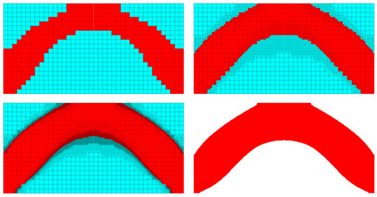
Figure 38. Selected middle topologies and the final one for the structure under self-weight. For the last iteration the grid has not been shown to improve the clarity of the picture.

8. Conclusions

The quality of structural topologies depends on the density of mesh discretization. On the other hand, the use of fine mesh for a whole structure in order to obtain a topology with smooth boundaries implies a high computational cost. The remedy for that can be the implementation of the adaptive mesh refinement. Refining mesh in an adaptive way allows for reduction of the number of elements without losing the accuracy of results. Choosing this approach in this paper, a Cellular Automata approach with the refined mesh adaptation has been proposed in order to generate structural topologies. The fine grid was implemented mainly in the so-called grey regions, where it has to be decided whether a cell becomes solid or void. The results of topology generation for illustrative examples confirmed the accuracy of the approach presented in this paper.

The benefits of applying the Cellular Automata algorithm with the refined mesh adaptation can be summarized as follows:

• high-resolution optimal topologies can be generated with a relatively low computational cost
• the algorithm presented is versatile, which allows for its easy combination with any solver built on a finite element method
• using Cellular Automata does not require additional density filtering
• boundaries of the resulting structures are smooth
• in the case of a fine mesh, thin and slender parts of structural topology do not appear
• the so-called grey areas are eliminated without using any additional filtering
• the mesh dependency phenomenon has not been observed
• topologies generated are free of the checkerboard effect.

Although the discussion in this paper has been restricted to generation of plane topologies, it has to be stressed that the proposed concept can be extended to spatial problems. Both the form of the Cellular Automata local rules and the possibility of refinement of the meshing procedure offered by the ANSYS solver allow adjustment to 3D tasks.

It is also worth noting that the proposed approach can also be extended to the implementation of the adaptive mesh refinement based on solution errors, e.g., equivalent stress error or deformation error, which allows for improvement in the numerical accuracy of the structural analysis.

References

- Lewiński, T.; Rozvany, G.I.N.; Sokół, T.; Bołbotowski, K. Exact analytical solutions for some popular benchmark problems in topology optimization III: L-shaped domains revisited. Struct. Multidisc. Optim. 2013, 47, 937–942. [Google Scholar] [CrossRef]
- Rozvany, G.I.; Sokół, T.; Pomezanski, V. Fundamentals of exact multi-load topology optimization—Stress-based least-volume trusses (generalized Michell structures)–Part I: Plastic design. Struct. Multidisc. Optim. 2014, 50, 1051–1078. [Google Scholar] [CrossRef]
- Bochenek, B.; Tajs-Zielińska, K. GHOST—Gate to Hybrid Optimization of Structural Topologies. Materials 2019, 12, 1152. [Google Scholar] [CrossRef] [PubMed]
- Maute, K.; Ramm, E. Adaptive topology optimization. Struct. Optim. 1995, 10, 100–112. [Google Scholar] [CrossRef]
- de Sturler, E.; Paulino, G.; Wang, S. Topology optimization with adaptive mesh refinement. In Proceedings of the 6th International Conference on Computation of Shell and Spatial Structures IASS-IACM 2008: “Spanning Nano to Mega”, Ithaca, NY, USA, 28–31 May 2008; Abel, J.F., Cooke, J.R., Eds.; Cornell Universit: Ithaca, NY, USA, 2012. [Google Scholar]
- Baiges, J.; Martínez-Frutos, J.; Herrero-Pérez, D.; Otero, F.; Ferrer, A. Large-scale stochastic topology optimization using adaptive mesh refinement and coarsening through a two-level parallelization scheme. Methods Appl. Mech. Eng. 2019, 343, 186–206. [Google Scholar] [CrossRef]
- Zhang, S.; Gain, A.; Norato, J. Adaptive Mesh Refinement for Topology Optimization with Discrete Geometric Components. arXiv 2019, arXiv:1910.05585. [Google Scholar] [CrossRef]
- Hoshina, T.Y.S.; Menezes, I.F.M.; Pereira, A. A simple adaptive mesh refinement scheme for topology optimization using polygonal meshes. J. Braz. Soc. Mech. Sci. Eng. 2018, 40, 1–17. [Google Scholar] [CrossRef]
- Nana, A.; Cuillière, J.C.; Francois, V. Towards adaptive topology optimization. Adv. Eng. Softw. 2016, 100, 290–307. [Google Scholar] [CrossRef]
- Lambe, A.B.; Czekanski, A.B. Topology optimization using a continuous density field and adaptive mesh refinement. Int. J. Numer. Meth. Eng. 2018, 113, 357–373. [Google Scholar] [CrossRef]
- Troya, M.; Tortorelli, D. Adaptive mesh refinement in stress-constrained topology optimization. Struct. Multidiscip. Optim. 2018, 58, 2369–2386. [Google Scholar] [CrossRef]
- Wang, Y.; Kang, Z.; He, Q. Adaptive topology optimization with independent error control for separated displacement and density fields. Comput. Struct. 2014, 135, 50–61. [Google Scholar] [CrossRef]
- Nguyen-Xuan, H. A polytree-based adaptive polygonal finite element method fortopology optimization. Int. J. Numer. Methods Eng. 2017, 110, 972–1000. [Google Scholar] [CrossRef]
- Egger, A.; Saputra, A.; Triantafyllou, S.; Chatzi, E. Exploring Topology Optimization on Hierarchical Meshes by Scaled Boundary Finite Element Method. In Proceedings of the International Conference on Computational Methods (Vol. 6, 2019) 10th ICCM, Singapore, 9–13 July 2019; Liu, G.R., Cui, F., Xu, G., Eds.; [Google Scholar]
- Michell, A.G.M. The limits of economy of material in frame structures. Philos. Mag. 1904, 8, 589–597. [Google Scholar] [CrossRef]
- Bendsoe, M.P.; Kikuchi, N. Generating optimal topologies in optimal design using a homogenization method. Comput. Methods Appl. Mech. Eng. 1988, 71, 197–224. [Google Scholar] [CrossRef]
- Bendsoe, M.P. Optimal shape design as a material distribution problem. Struct. Optim. 1989, 1, 193–200. [Google Scholar] [CrossRef]
- Bendsoe, M.P. Optimization of Structural Topology, Shape and Material, 1st ed.; Springer: Berlin/Heidelberg, Germany, 1995. [Google Scholar] [CrossRef]
- Zhou, M.; Rozvany, G.I.N. The COC algorithm, part II: Topological, geometry and generalized shape optimization. Comput. Methods Appl. Mech. Eng. 1991, 89, 197–224. [Google Scholar] [CrossRef]
- Bendsoe, M.P.; Sigmund, O. Topology Optimization. Theory, Methods, and Applications, 2nd ed.; Springer: Berlin/Heidelberg, Germany, 2004. [Google Scholar] [CrossRef]
- Allaire, G.; Jouve, F.; Toader, A.M. A level-set method for shape optimization. C. R. Math. 2002, 334, 1125–1130. [Google Scholar] [CrossRef]
- Allaire, G.; Jouve, F.; Toader, A.M. Structural optimization using sensitivity analysis and a level-set method. J. Comput. Phys. 2004, 194, 363–393. [Google Scholar] [CrossRef]
- Xie, Y.M.; Steven, G.P. A simple evolutionary procedure for structural optimization. Comput. Struct. 1993, 49, 885–896. [Google Scholar] [CrossRef]
- Von Neumann, J. Theory of Self-Reproducing Automata; University of Illinois Press: Urbana, IL, USA, 1966. [Google Scholar]
- Ulam, S. Random processes and transformations. In Proceedings of the International Congress of Mathematics, Cambridge, UK, 30 August–6 September 1950; Volume 2, pp. 85–87. [Google Scholar]
- Tovar, A.; Patel, N.; Kaushik, A.K.; Letona, G.; Renaud, J.; Sanders, B. Hybrid Cellular Automata: A biologically-inspired structural optimization technique. In Proceedings of the 10th AIAA/ISSMO Multidisciplinary Analysis and Optimization Conference, Albany, NY, USA, 30 August–1 September 2004; p. 15. [Google Scholar] [CrossRef]
- Bochenek, B.; Tajs-Zielinska, K. Novel local rules of cellular automata applied to topology and size optimization. Eng. Optim. 2012, 44, 23–35. [Google Scholar] [CrossRef]
- Zeng, D.; Duddeck, F. Improved hybrid cellular automata for crashworthiness optimization of thin-walled structures. Struct. Multidiscip. Optim. 2017, 56, 101–115. [Google Scholar] [CrossRef]
- Tovar, A.; Quevedo, W.I.; Patel, N.M.; Renaud, J.E. Topology optimization with stress and displacement constraints using the hybrid cellular automaton method. In Proceedings of the Third European Conference on Computational Mechanics, Solids, Structures and Coupled Problems in Engineering, Lisbon, Portugal, 5–8 June 2006; Springer: Berlin/Heidelberg, Germany, 2006. [Google Scholar]
- Bochenek, B.; Tajs-Zeilinska, K. GOTICA-generation of optimal topologies by irregular cellular automata. Struct. Multidiscip. Optim. 2017, 55, 1989–2001. [Google Scholar] [CrossRef]
- Inou, N.; Shimotai, N.; Uesugi, T. A cellular automaton generating topological structures. In Proceedings of the 2nd European Conference on Smart Structures and Materials, Glasgow, UK, 12–14 October 1994; Volume 2361, pp. 47–50. [Google Scholar] [CrossRef]
- Bochenek, B.; Tajs-Zielińska, K. Topology optimization with efficient rules of cellular automata. Eng. Comput. 2013, 30, 1086–1106. [Google Scholar] [CrossRef]
- Bochenek, B.; Mazur, M. A novel heuristic algorithm for minimum compliance optimization. Eng. Trans. 2016, 64, 541–546. [Google Scholar]
- Li, S. Comparison of refinement criteria for structured adaptive mesh refinement. J. Comput. Appl. Math. 2010, 233, 3139–3147. [Google Scholar] [CrossRef]
- Andreassen, E.; Clausen, A.; Schevenels, M.; Lazarov, B.S.; Sigmund, O. Efficient topology optimization in MATLAB using 88 lines of code. Struct. Multidisc. Optim. 2010, 43, 1–16. [Google Scholar] [CrossRef]
- Bruns, T.E.; Tortorelli, D.A. Topology optimization of non-linear elastic structures and compliant mechanisms. Comput. Methods Appl. Mech. Eng. 2001, 190, 3443–3459. [Google Scholar] [CrossRef]
- Biyikli, E.; To, A.C. Proportional topology optimization: A new non-sensitivity method for solving stress constrained and minimum compliance problems and its implementation in Matlab. PLoS ONE 2015, 10, 1–23. [Google Scholar] [CrossRef]
- Wang, H.; Liu, J.; Wen, G. An adaptive mesh-adjustment strategy for continuum topology optimization to achieve manufacturable structural layout. Numer. Methods Eng. 2019, 117, 1304–1322. [Google Scholar] [CrossRef]
- Bruyneel, M.; Duysinx, P. Note on Topology Optimization of Continuum Structures Including Self Weight. Struct. Multidisc. Optim. 2005, 29, 245–256. [Google Scholar] [CrossRef]
- Tajs-Zielinska, K.; Bochenek, B. A Heuristic Approach to Optimization of Structural Topology Including Self-Weight. AIP Conf. Proc. 2018, 1922, 020001. [Google Scholar] [CrossRef]
- Felix, L.; Gomes, A.; Suleman, A. Wing topology optimization with self-weight loading. In Proceedings of the 10th World Congress on Structural and Multidisciplinary Optimization, Orlando, FL, USA, 19–24 May 2013; Furnish, M.D., Ed.; [Google Scholar] [CrossRef]
© 2020 by the authors. Licensee MDPI, Basel, Switzerland. This article is an open access article distributed under the terms and conditions of the Creative Commons Attribution (CC BY) license (http://creativecommons.org/licenses/by/4.0/).