Article

Improved U-Net: Fully Convolutional Network Model for Skin-Lesion Segmentation

The School of Computer Science and Engineering, Kyungpook National University, Daegu 41566, Korea
*
Authors to whom correspondence should be addressed.
Appl. Sci. 2020, 10(10), 3658; https://doi.org/10.3390/app10103658
Submission received: 23 March 2020 / Revised: 20 May 2020 / Accepted: 22 May 2020 / Published: 25 May 2020

Abstract

:
The early and accurate diagnosis of skin cancer is crucial for providing patients with advanced treatment by focusing medical personnel on specific parts of the skin. Networks based on encoder–decoder architectures have been effectively implemented for numerous computer-vision applications. U-Net, one of CNN architectures based on the encoder–decoder network, has achieved successful performance for skin-lesion segmentation. However, this network has several drawbacks caused by its upsampling method and activation function. In this paper, a fully convolutional network and its architecture are proposed with a modified U-Net, in which a bilinear interpolation method is used for upsampling with a block of convolution layers followed by parametric rectified linear-unit non-linearity. To avoid overfitting, a dropout is applied after each convolution block. The results demonstrate that our recommended technique achieves state-of-the-art performance for skin-lesion segmentation with 94% pixel accuracy and a 88% dice coefficient, respectively.

1. Introduction

Melanoma is one of the most serious skin ailments worldwide, accumulating 287,723 new cases and over 60,000 estimated fatalities in 2018 [1]. Skin cancer is one of the most significant public health issues, with over 2000 new diagnoses in South Korea just in the past 5 years [2]. New melanoma arising on the skin surface can be easily identified via visual inspection. Unfortunately, most melanomas are not noticed in a timely manner by sufferers [3]. Nevertheless, individual visual inspection by professional dermatologists provides a diagnostic accuracy of ~60%, which means many potentially treatable melanomas are not detected until they are quite advanced [4]. The accurate and early segmentation of skin lesions is critical to the detection and localization of visual dermoscopic features of the skin and the classification of skin-based diseases. Dermoscopy is an imaging technique that decreases the surface reflection of skin, allowing deeper layers to be visually inspected. It is used to improve diagnostic performance and minimize melanoma deaths. Figure 1 displays a few dermoscopic images of melanoma skin lesions.
The deep-learning community has applied various techniques to boost traditional computer-vision activities by utilizing neural networks. Hence, convolutional neural networks (CNN) have revolutionized image classification, scene identification, target recognition, and other capabilities because of their ability to build inner descriptions of images. CNN-based approaches are much better than other technologies for comprehending location and dimension in various forms. CNNs have led to vast improvements in task recognition. Apart from enhancing image classification tasks [5,6,7], they have also gained ground in regional tasks requiring organized results. Such advancements have been made in object detection [8,9,10], part and key-point prediction [11,12] and local correspondences [11,13]. CNNs are used for current semantic segmentation techniques [14,15,16,17,18,19], in which every pixel is classified according to its nearby object or region. Indeed, this is essential when dealing with medical images. Consistent image segmentation is a very important task, and successfully enabling diagnostic capability is the main objective of medical image segmentation, which is principally a pixel-level classification problem.
Fully convolutional networks (FCN) are one of the successful methods among the initially proposed neural networks for image segmentation [5]. By applying FCNs to CNN technology, feature to feature mapping can be achieved without first obtaining spatial information [20,21,22,23,24]. The FCN architecture is a broadened type of CNN and contains only convolutional and pooling layers, which provide the ability to make predictions about inputs. These are generally applied to local tasks instead of global ones [25,26]. A variety of FCN-based methods have been suggested recently to mitigate this problem. For example, the author of [27] suggested a multi-scale CNN that contained sub-networks having different resolution results to gradually expand coarse estimation.
In order to reconstruct accurate forms of target borderlines, sort pixel-wise class labels and calculate segmentation masks, the straightforward deconvolutional step has been replaced with a deep up-convolution network in [28]. Several studies tried to achieve better segmentation accuracy by using spatial information. U-Net has achieved great performance through skip connections by joining features of low-level layers and high-level layers [29].
The foremost weakness of the U-Net architecture is that training may reduce the training speed in the middle layers of deeper neural networks, so there is the threat of overlooking the layers. The main reason for this phenomenon is that gradients become weakened further away from the output layer of a network, where the loss of the training is computed. Additionally, the rectified linear unit (ReLU) activation function was used in the original U-Net paper. The dead neuron problem of the ReLU has been detected by Lu et al. [30]. We substituted ReLU activation function with PReLU non-linearity for training the network to lessen the effect of this problem.
The foremost responsibility of activation functions is to convert an input signal of a layer in the neural network to an output signal. A rectified linear unit (ReLU) is the key activation function for this activity in deep-neural networks [31]. It expedites the convergence of the training procedure and produces better results compared with standard sigmoid-like activation functions. Apart from the numerous benefits of a ReLU rectifier, recent studies have shown that there are shortcomings [30,32].
The main downside of U-Net is that training can decelerate in the intermediate layers of deeper networks. Thus, there is risk of ignoring layers where abstract attributes are exemplified. This is caused by gradients becoming weakened farther away from the last layer of the network, where the difference between predicted and actual values is calculated, causing slower updates for far-removed weights. Another limitation is that the classic deconvolutional method of generating images, achievements notwithstanding, has produced theoretical concerns that direct artifacts are sometimes produced in images. In our approach, we apply an interpolation method for upsampling to overcome these problems. We achieve an adequate accuracy for skin-lesion segmentation because of the aspects of the bilinear interpolation and a parametric ReLU (PReLU) nonlinearity, which admirably matches the chosen interpolation method.
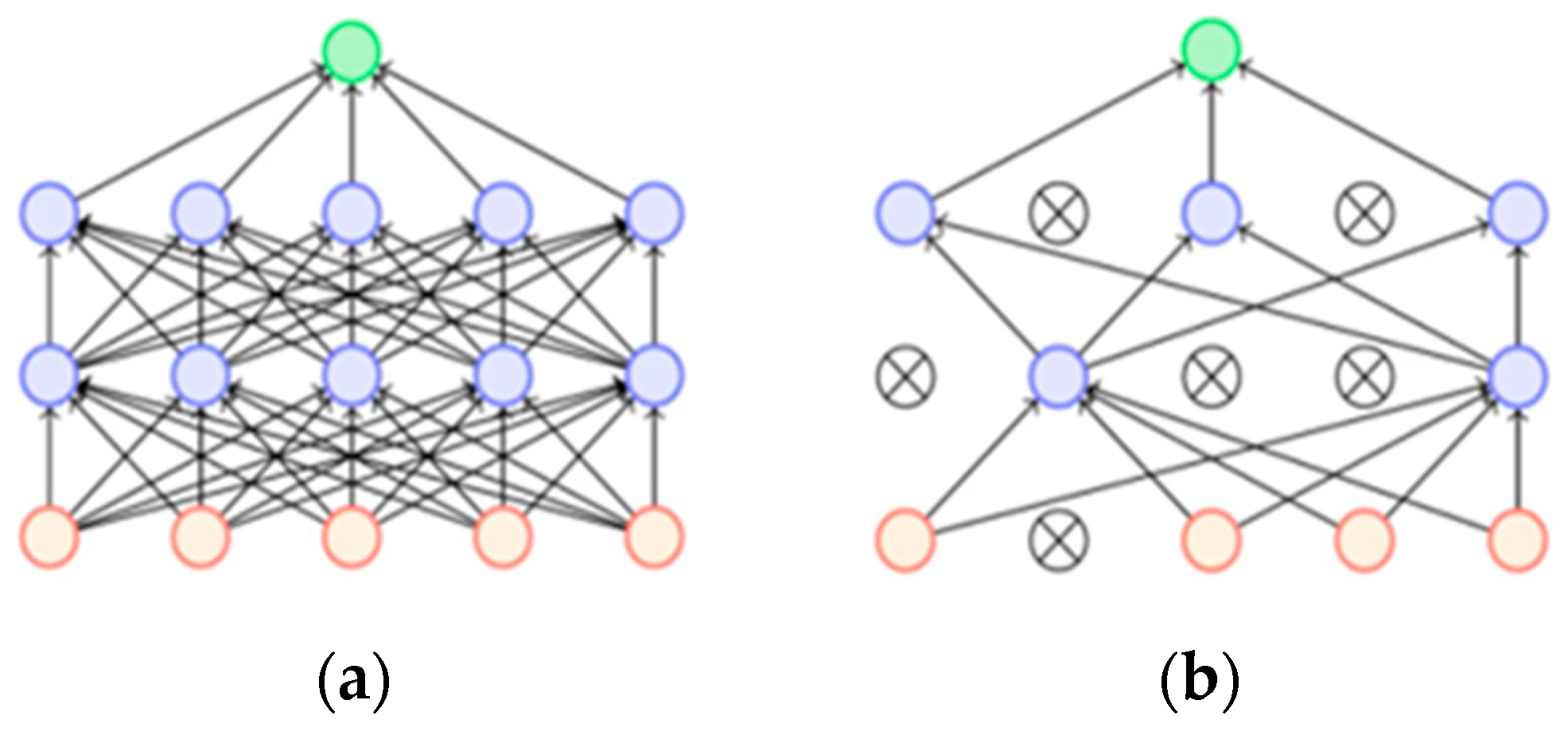
Deep-neural networks include multiple nonlinear concealed layers, leading to expressive models learning very complex relations between inputs and results. With restricted training data, many of these complex relationships will refer to noise, which leads to overfitting. Several approaches have been applied to avoid this. Strivastava et al. proposed a dropout method to mitigate this problem. The technique randomly drops units from the neural network during training [33]. This prevents excessive perfect co-adaptations. More technically, individual nodes are either dropped from the net with probability of 1 p or kept with probability of p . The reduced network is then left for training while the inputs and outputs for the dropped-out nodes are eliminated, as illustrated in Figure 2.
The main purpose of this paper is achieving an adequate accuracy for skin-lesion segmentation because of the aspects of the bilinear interpolation and a parametric ReLU (PReLU) nonlinearity, which admirably matches the chosen interpolation method. In order to avoid overfitting and speeding up the training step, we use a dropout technique after convolutional layers.

2. Materials and Methods

2.1. Overview

We propose a novel neural-network architecture that can overcome uneven overlapping and fading gradients in the intermediate layers. The key advantage of this recommended architecture over the classical U-Net framework entails its upsampling stage. The attained segmentation accuracy is commensurate-to-slightly-better-than that accomplished using the standard U-Net architecture. Furthermore, its accuracy is increased, reducing segmentation artifacts. Our modified architecture is also more computationally effective than the standard transposed convolutional U-Net method. The proposed method has been trained with the following system configuration: a Intel(R) Core (TM) i7-9700K processor, 32 GB of installed memory (RAM) and an 8 GB NVIDIA GeForce RTX 2060 SUPER graphics card.

2.2. Dataset

We use the dataset reported in [34], which contains both training and testing data. The training dataset includes 2594 dermoscopic skin-lesion images and corresponding ground-truth response masks. The testing dataset consists of 1000 images. Originally, every image in both the training and testing sets is of different size. First, images should be equal in size and grayscale. We thus resized all the input images to 256 × 256 and converted them to binary prior to training. Second, normalization must be applied before training. For image normalization, the matrices representing training and testing were divided by 255 to place them in the range (0, 1). We then split the training dataset into training and validation at 90% and 10%, respectively.

2.3. Proposed Method Architecture

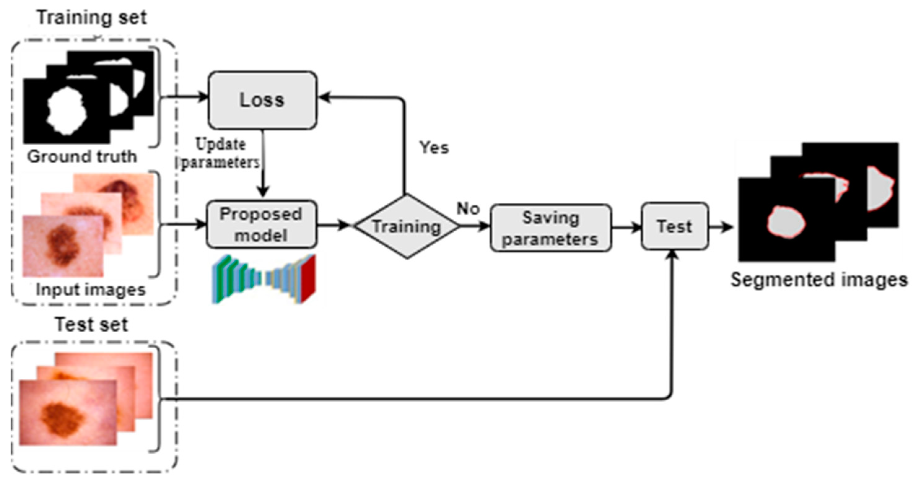
Figure 3 provides a general flowchart of our image segmentation model, through which the input images transit. The initial training step is executed automatically by default. The binary cross-entropy loss function is computed by comparing the ground truth with the resultant image segmentation. This procedure is repeated until the properties of the callback function are satisfied during training. At each iteration, the weights and biases are updated via backpropagation. When training is complete, the model checkpoints save the final parameter values. These weight values and biases are then used for testing unseen images.
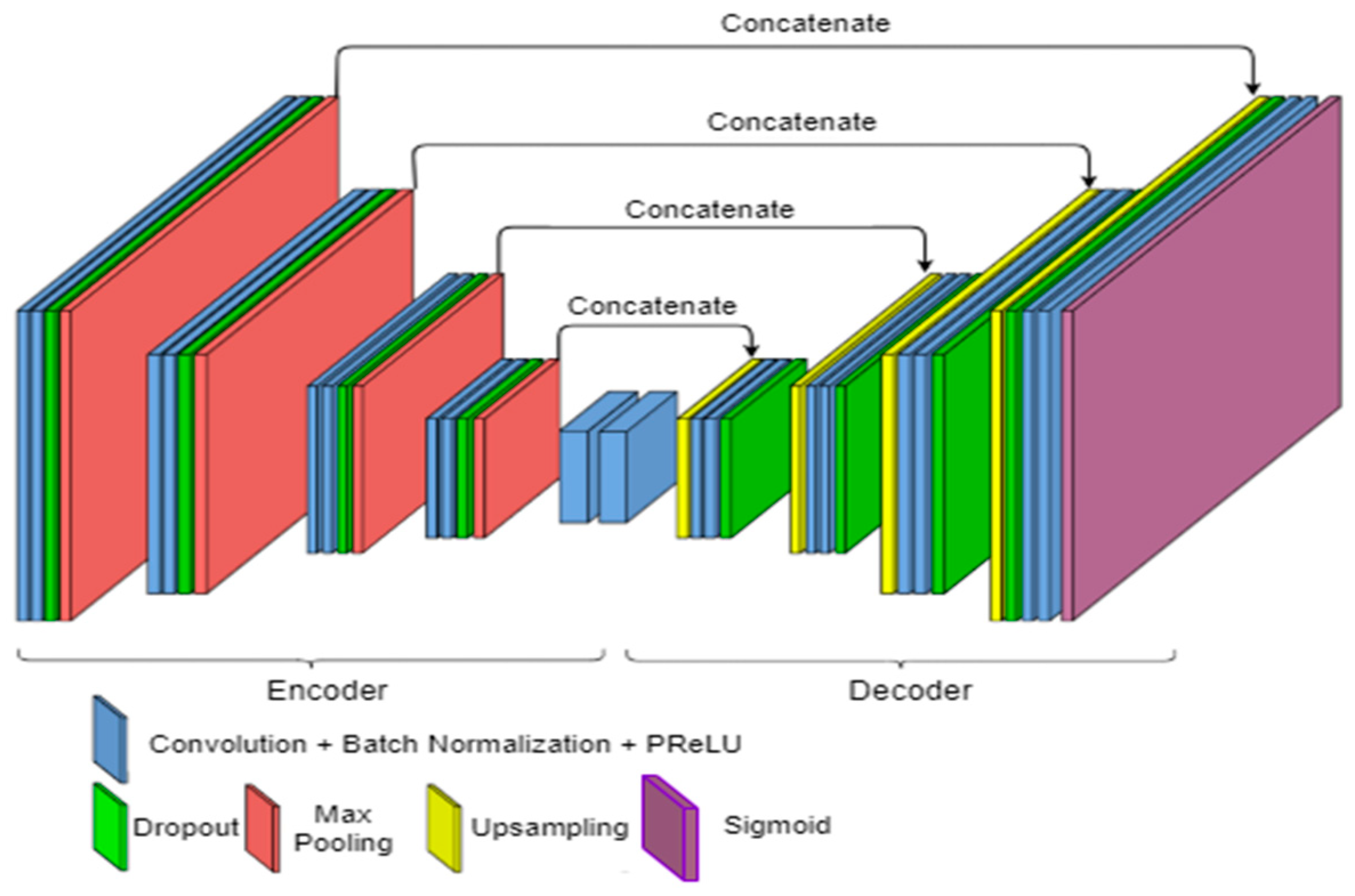
In Figure 4, the model architecture consists of two paths: encoder (left side) and decoder (right side). The encoder path operates like a classic CNN. It includes joint 3 × 3 convolutions with batch normalization, followed by a PReLU activation function. In every down-sampling step, we have two convolution layers. To avoid overfitting, the dropout method is used before applying a max-pooling operation. The channel size is increased twice at each down-sampling step so that the size of the feature map declines.
The most important path in CNN-based image segmentation is that of the decoder. At each decoder path step, a 2 × 2 bilinear interpolation is applied for upsampling the feature map. To reform the spatial data, the result of the decoder path and the correspondingly cropped feature map from the encoder feature map are merged and tracked by again operating the same-size convolution layers, batch normalization, and PReLU nonlinearity. A 1 × 1 convolution is used for the final layer to record each feature vector tailed with its sigmoid activation function for extracting the binary image. In the next sub-sections, we discuss the techniques used in the network architecture.

2.4. Upsampling Method

U-Net normally includes two sections: downsampling and upsampling. The authors of [29] attained accurate pixel-level localization by concatenating the downsampling and upsampling layers together. Upsampling is the most important part of the U-Net architecture, because the spatial information of the feature map is generated here. Transpose convolution (or deconvolution), having learnable parameters, is used in the upsampling section. Apart from its learnable parameters, this execution method is very time-consuming, because the kernels require additional weights for training. Moreover, it can lead to uneven overlap [35], as depicted by the checkerboard pattern of Figure 5, which causes artifacts at a variety of scales.
We use bilinear interpolation, an alternative to standard deconvolution, in the decoder part of our model to avoid artifacts. In contrast to deconvolution, this method does not have artifacts because of its default behavior. The image coordinates, f ( n 10 , n 20 ) , f ( n 11 , n 21 ) , f ( n 12 , n 22 ) and f ( n 13 , n 23 ) , are the nearest neighbors of g ( n 1 , n 2 ) . The intensity values of the interpolated image g ( n 1 , n 2 ) are computed as follows:
g ( n 1 , n 2 ) = A 0 + A 1 n 1 + A 2 n 2 + A 3 n 1 n 2
Equation (1) represents a bilinear function having coordinates ( n 1 , n 2 ) . Here, we refer to f as an intensity value at given ( n 10 , n 20 ) ,   ( n 11 , n 21 ) , ( n 12 , n 22 ) and ( n 13 , n 23 )   pixel locations before applying interpolation and g as an intensity value of interpolated image matrix in ( n 1 , n 2 ) coordinates, and A s are the bilinear weights. The bilinear weights, A 0 , A 1 , A 2 and A 3 , are computed by solving the matrix in Equation (2):
[ A 0 A 1 A 2 A 3 ] = [ 1 n 10 1 n 11 n 20 n 10 n 20 n 21 n 11 n 21 1 n 12 1 n 13 n 22 n 12 n 22 n 23 n 13 n 23 ] 1 [ f ( n 10 , n 20 ) f ( n 11 , n 21 ) f ( n 12 , n 22 ) f ( n 13 , n 23 ) ]
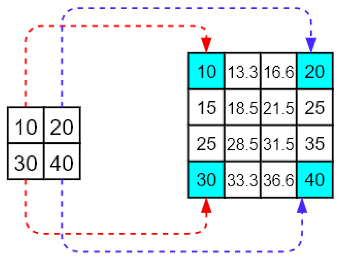
As a result, g ( n 1 , n 2 ) is defined as a linear combination of the gray levels of its four nearest neighbors. The linear combination defined by Equation (1) is, in fact, the value assigned to g ( n 1 , n 2 ) when the perfect least-squares planar fit is made to these four neighbors. This process of optimal averaging produces smoother results. In Figure 6, we visually describe bilinear interpolation.
In this example, we increase the size of the 2 × 2 matrix into a 4 × 4 one. According to Equation (2), the weight values of specific elements in the up-sampled matrix depend on how near this element is to known elements.
Transpose convolution has learnable parameters for training. The number of parameters is more than 10 million in deep-neural networks, such as U-Net, because of their trainable weight and bias values in transpose convolution. Consequently, this causes adverse impacts triggered by voiding the middle layers’ gradients of the U-Net models. We achieve a reduction of this detrimental impact by applying bilinear interpolation to the decoder part.

2.5. Activation Functions

2.5.1. ReLU

Activation functions are key to artificial neural networks discovering and making sense of complex and nonlinear relationships between input and output, because they bring nonlinearity to the network. Their objective is to convert an input signal layer of the neural network into an output signal. The ReLU is the most common activation function in deep networks. It expedites the convergence of the training procedures and provides better results compared with standard sigmoid-like activation functions [36,37,38]. The function and derivative of this nonlinearity are represented as follows:
f ( x ) = {   x i f x 0 0 i f x < 0 f ( x ) = {   1 i f x > 0 0 i f x < 0 ( a )   Function ( b )   Derivative
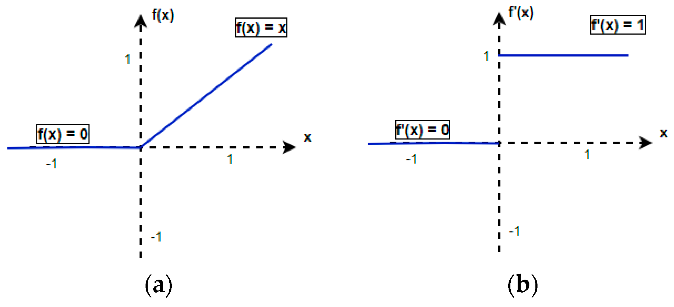
Geometrically, the ReLU function and its derivative are illustrated as follows:
The ReLU is linear for all non-negative values and zero otherwise. The derivative, an important factor for updating gradients, is zero when it takes negative values and one otherwise. Apart from the numerous benefits of the ReLU rectifier, recent studies show that there are some shortcomings [39,40]. Several gradients can be unstable during training and can “die” by causing a weight to update in such a way that it will never activate on any data point again. Thus, the ReLU can result in “dead neurons”. For activations in the region (x < 0) of the ReLU, the gradient will be zero, and the weights 0 will not be fine-tuned during descent. Thus, the neurons that go into that state will stop responding to variations in the input. Simply because the gradient is zero, nothing will change. This is called the “dying ReLU” problem [30,32].
Systems using these units sometimes manifest the dying ReLU issue during training, in which the state (x < 0) is very likely for most training examples for nodes within the network. It is comprehensible that the error backpropagation algorithm utilizes a derivative function, f’(x), such that the ReLU nonlinearity is zero for x < 0 (see Figure 7). Thus, patterns that cause x < 0 do not change the unit’s parameters. This condition can cause ambiguity in practice, because units that are not active will probably not be trained. The dying ReLU problem is likely to occur when:
  • The learning rate is too high.
  • There is a large negative bias.
Consider the following equation used to update the weight values during backpropagation:
w n e w = w o l d ( ծ L ծ w ) α + b .
Here, α is the learning rate, b is the bias, and ծ L ծ w is the derivative of the loss function with respect to the weight value (w). Thus, if the learning rate is too high or the bias is negative, it may bring negative new weight values after the backpropagation step. After the weight becomes negative, the ReLU activation function of that neuron will never be activated and will lead to the death of the neuron.

2.5.2. PReLU

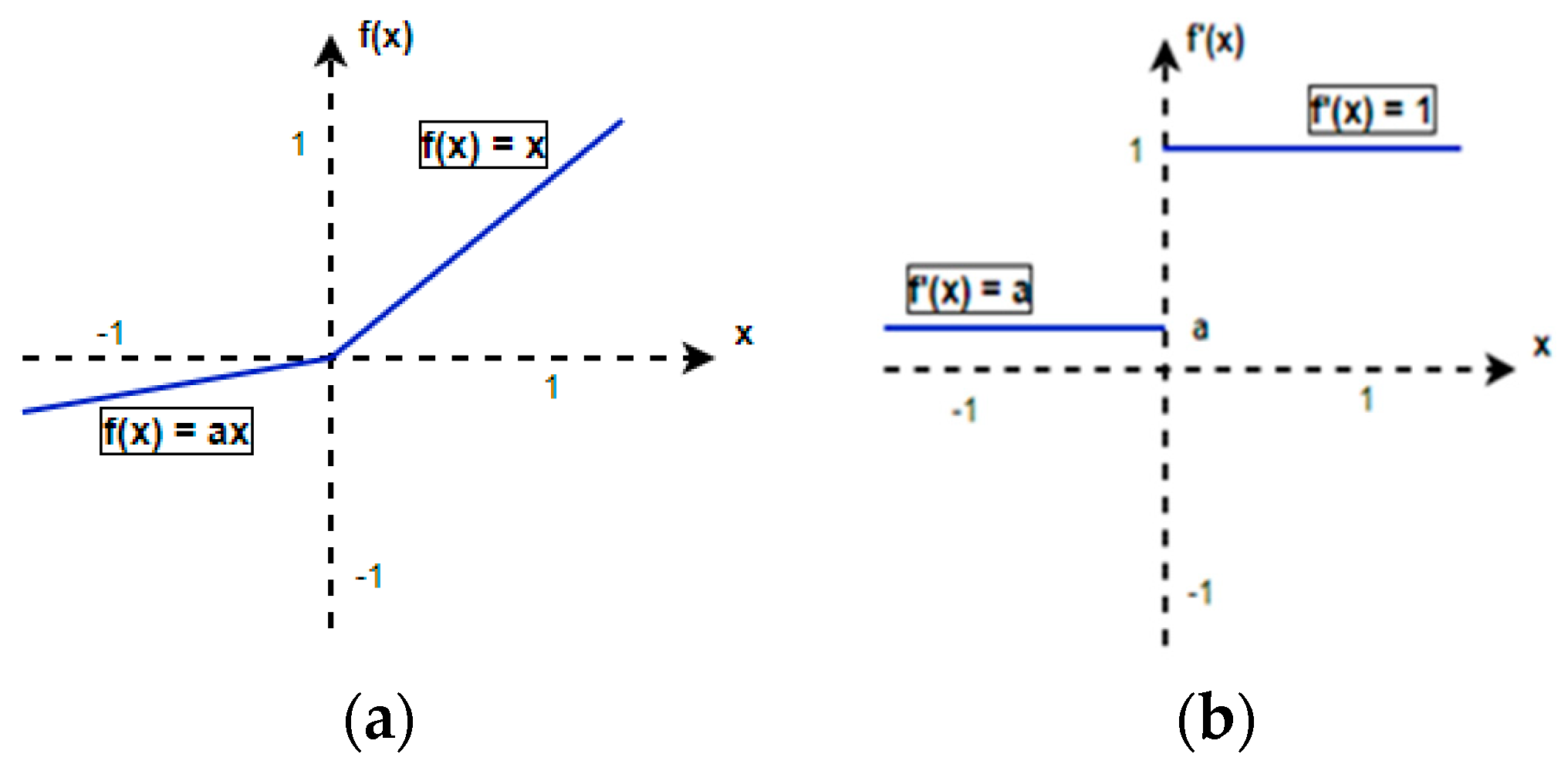
To overcome the downsides of ReLU nonlinearity, the PReLU has been introduced. This is a new generalization of the ReLU, in which the activation function adaptively learns the parameters of the rectifiers and increases accuracy at little additional computational cost. The PReLU attempts to fix the dying ReLU problem by providing a slight negative slope when the input values are negative. This activation function allows the neurons to decide the most correct slope for the negative region. The formal definition of the PReLU and its derivative are given below:
f ( x i ) = { x i i f x i a i x i     i f     x i < 0 f ( x i ) = {   1     i f     x i > 0 a i     i f     x i < 0 ( a )   PReLU   activation   function ( b )   Derivative   of   PReLU
In Equation (5), x i is the input of the activation function, f, in the i th node, and a i is a coefficient managing the angle of the negative section that allows the nonlinearity to differ at each node. When a i = 0, it becomes a ReLU. If a i is small and remains the same value, the ReLU becomes a “leaky” ReLU and has an insignificant impact on precision. If a i is a learnable parameter of the network, the equation becomes a PReLU. Figure 8 shows the PReLU activation function.
In the PReLU, the alpha parameter (i.e., the “leak”) is included to prevent the gradient from becoming zero. This makes the gradient more robust for optimization, because the weight is adapted for those neurons that are not active within the ReLU. The PReLU has non-constant coefficients in its negative part, and these are adaptively learned by the model. Taking all benefits of the PReLU into consideration, we use this activation function for our proposed neural network.

3. Experimental Settings

3.1. Training Network

Convolutions of 3 × 3 were applied to each convolution layer followed by the PReLU and max pooling with a size of 2 × 2 and a stride of 2. Sixteen filters were used for the first hidden layer. This number was doubled for each consecutive hidden layer until the end of the encoder path. This caused an increase in the number of channels and a decrease in the size of feature map. The volume of the feature map in the bottleneck (the part of the network between the encoder and decoder path) was 16 × 16 with 256 channels. A 2 × 2 interpolation operated in the decoder path simultaneously enlarged the size of the feature map and decreased the number of channels. After each upsampling process, the convolution layer and the PReLU nonlinearity was utilized again. The predicted output size was the same as the input size: 256 × 256. Overall, the network contained more than 7 million trainable parameters. Batch normalization was used to normalize the input layer by adjusting and scaling the activations. Additionally, this permitted each layer of the network to learn by itself, separately from other layers.

3.2. Data Augmentation

The demand for biomedical image data is always high. Data augmentation is a tactic that allows the deep-learning community to significantly increase the diversity of data available for training without collecting new images. The size of the training dataset used in our work was insufficient for satisfactory training. Thus, we implemented data augmentation for the training set with horizontal flipping and a 20% rotation range. This way, we prevented our network from learning irrelevant features and essentially boosted the overall performance.

3.3. Evaluation Metrics

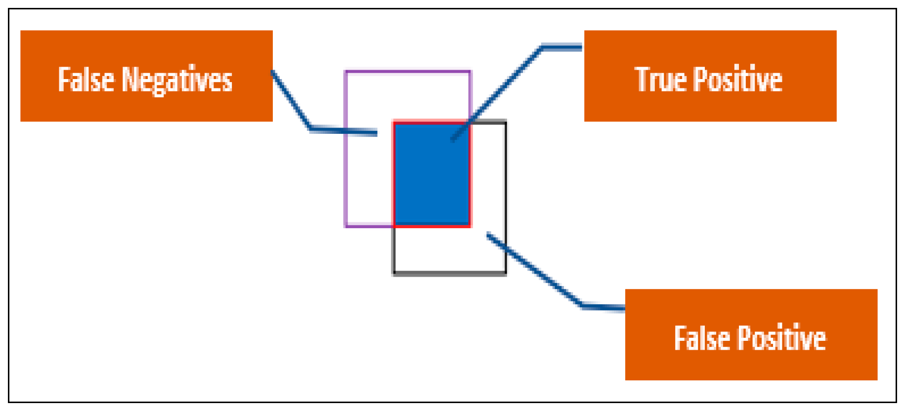
Ground truth is represented by the segmentation region defined by individual experts. The deep-neural network output is the segmentation result of the identical image generated by the deep-learning algorithm. The area of overlap defines how the two factors are matched with each other, and this area represents true positives (TP). False negatives result from the difference between the ground truth and TP. The remaining part of the union comprises false positives. Another part of the image that is not predicted by segmentation contains the true negatives. Figure 9 illustrates the above-mentioned terms geometrically.
To measure our method’s performance, we used three types of metric: the dice coefficient (DC), intersection-over-union (IOU), and pixel accuracy. The IOU metric (i.e., the Jaccard index) identifies the percentage overlap between the actual mask and our output prediction. Using the terms in Figure 9, we define IoU as
I o U = T P T P + F P + F N
Similarly, the DC can be written as
D i c e = 2 T P ( T P + F P ) + ( T P + F N )
An alternative metric used to assess semantic segmentation calculates the percentage of pixels in the image that were precisely classified. This pixel accuracy (PA) is usually reported independently for each class as well as globally for all classes:
P A = T P + T N T P + T N + F P + F N

4. Results and Discussion

When we compared our recorded result with different U-Net methods such as the original U-Net, FCN-1 (U-Net with the PReLU and transpose convolution), and FCN-2 (U-Net with the PreLU and bilinear interpolation), we achieved acceptable metrics accuracy with the test dataset. Table 1 shows the average accuracies over different models. Via experiments, we identified that using bilinear interpolation jointly with the PreLU was an effective method for skin-lesion segmentation. The training time per epoch is around 6 min for the original U-Net, and the proposed method spends less than 5 min per epoch.
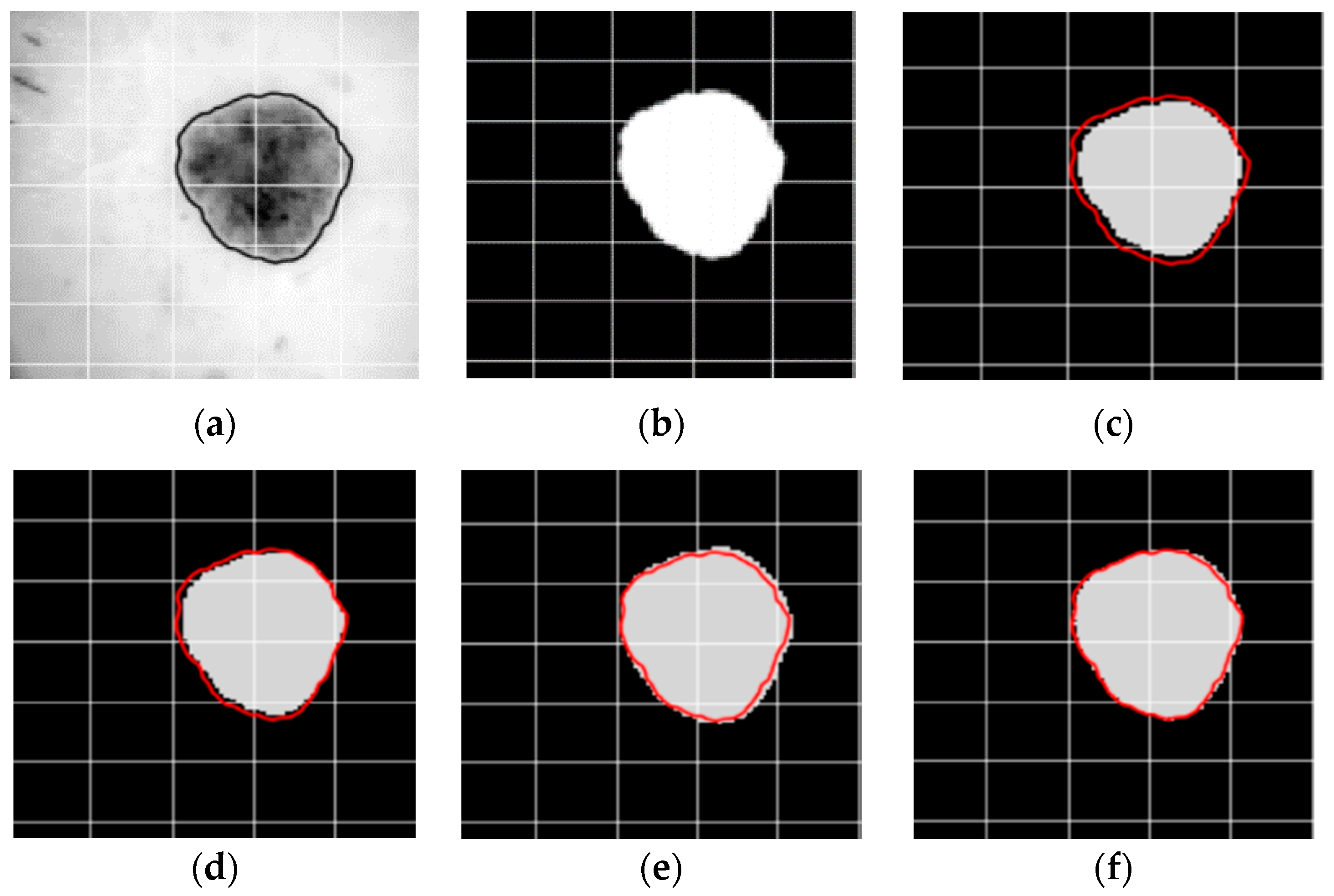
Figure 10 depicts image differences from the above-given versions of U-Net. The transpose convolution method for upsampling had more false negative results in the validation set. The experiments showed that a slight underfitting was recorded in the case of using transpose convolution (see Figure 10c,d). When the interpolation method was used with PreLU nonlinearity, the model detected more outliers in the validation set images. Figure 10e shows an image of high variance (overfitting). After applying the dropout technique, we overcame this problem in the interpolation method. The final visual result of the model is given in Figure 10f.
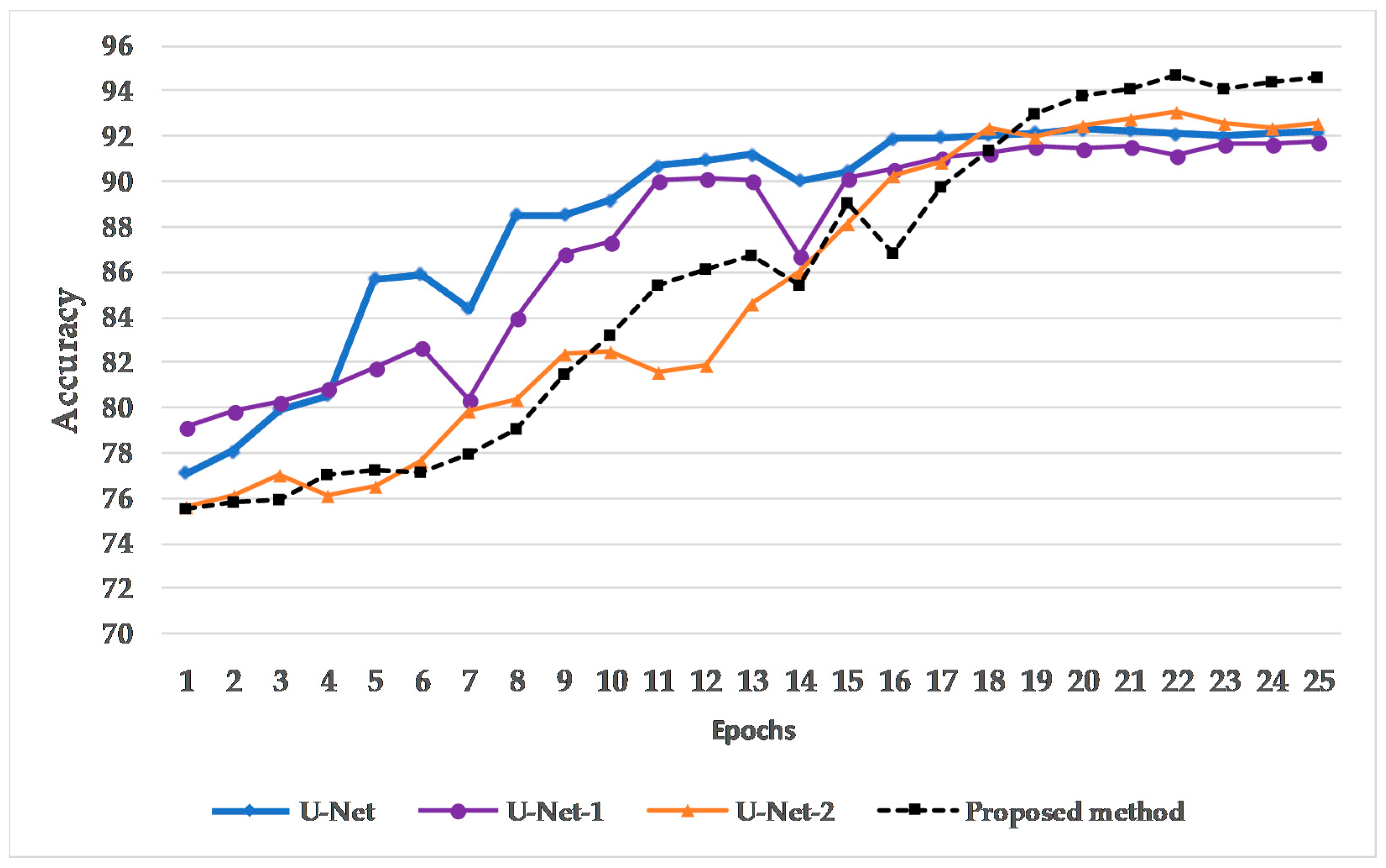
We compared the validation set accuracies of each model during training (see Figure 11). After 20 training epochs, the validation accuracy of each method remained nearly the same. In Figure 11, U-Net-1 and U-Net-2 reflect FCN-1 and FCN-2, respectively.
The illustration in Figure 11 helps us reach a conclusion about the learning procedure of each method. Transpose convolution-based models tend to learn faster, compared with interpolation-based methods. They almost always achieve their highest accuracy after 12 epochs. Contrarily, interpolation-based methods take much more time to achieve desired accuracies. The reason for this phenomenon is that the dropout effect causes a delay in reaching the desired accuracy. Another explanation for why bilinear interpolation-based approaches (FCN-2 and the proposed method) tend to learn more slowly than transpose convolution-based methods (U-Net and FCN-1) is that transpose convolution uses more learnable parameters compared with interpolation methods. In the initial steps of learning, transpose convolution-based methods try to learn with higher accuracy because of their default parameters. On the other hand, interpolation-based methods do not use learnable weights and biases. Therefore, they start to learn with lower accuracy and slowly reach the desired accuracy.
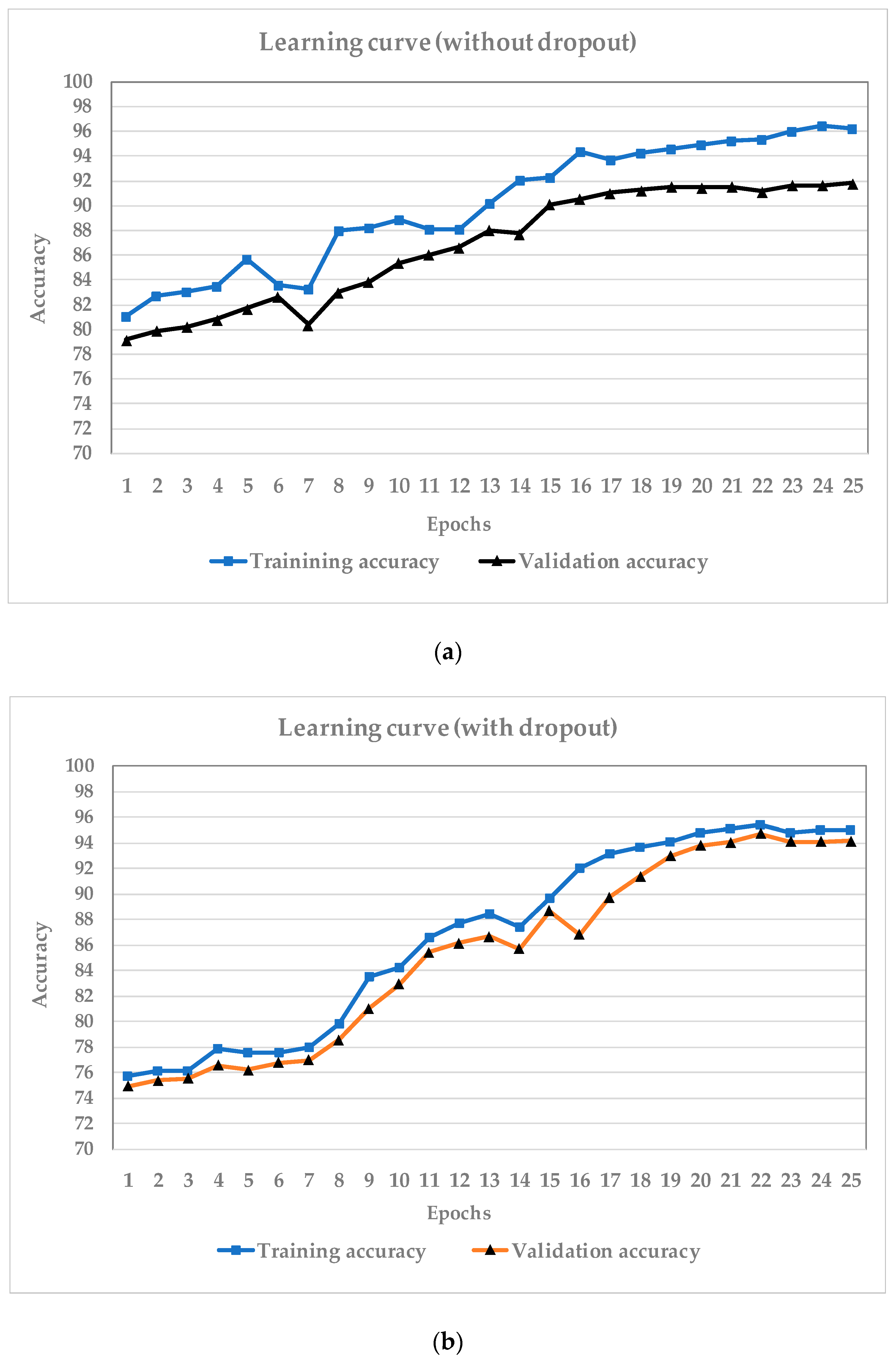
The graphs in Figure 12 clarify the training and validation accuracies of our technique. There is not much difference between training and validation accuracy, owing to the dropout regularization applied to the network.
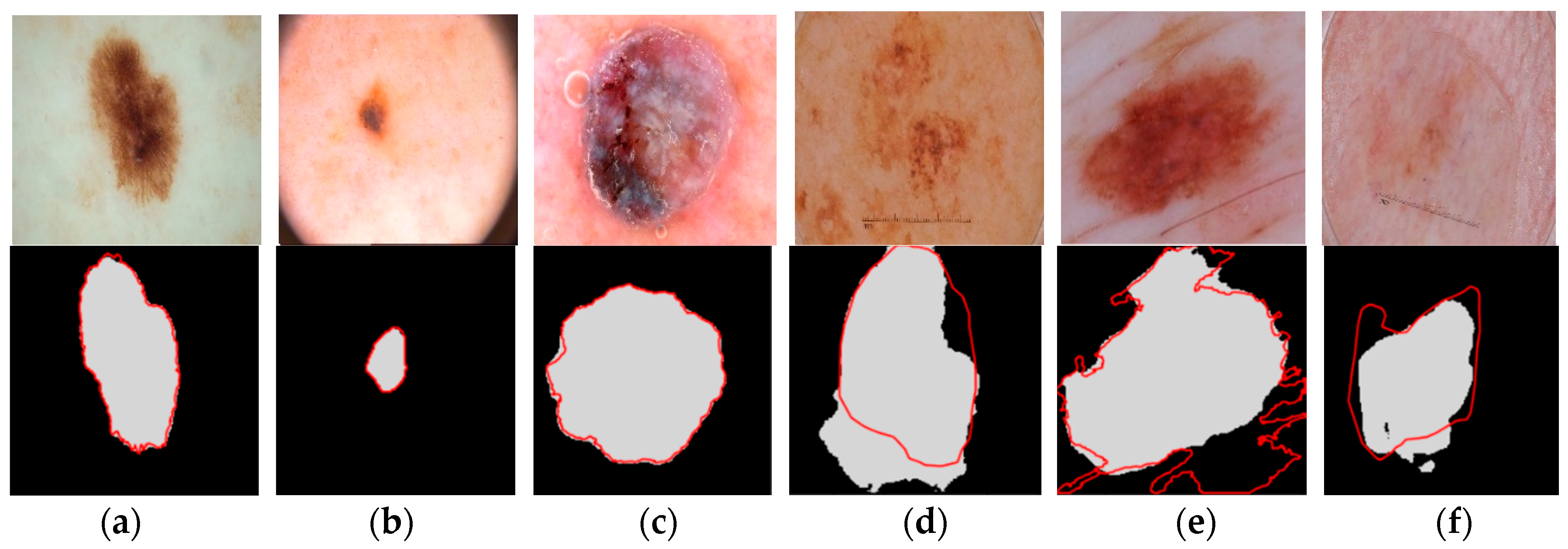
The overall dice coefficient was determined by calculating the average means of the individual dice coefficients of all images. Some DC values were relatively small because of noise in the input image. Another reason for the less DC values is that the skin and lesion colors are similar to each other in some test sample images. Consequently, there is the emergence of similar pixel intensities in those sample images. Figure 13 illustrates several examples of high and low dice coefficients in the validation set.

5. Conclusions and Future Work

In this paper, we used a bilinear interpolation method for the upsampling part of our FCN with a block of convolution layers. Our proposal approach provided good results for skin-lesion segmentation by jointly applying the PReLU and bilinear interpolation methods. We successfully eliminated artifacts caused by theoretical issues and reduced the detrimental impacts of U-Net parameters by using the interpolation method in the decoder part. To avoid overfitting, dropout was applied after each convolution block. We achieved ~94% PA and an 88.33% dice coefficient for skin-lesion segmentation. In future work, we plan to determine the reasons for low dice coefficients in some of our experimental cases by applying advanced image-processing techniques.

Author Contributions

Conceptualization, K.S.; data curation, O.B.; formal analysis, J.K. (Jaesoo Kim); funding acquisition, J.K. (Jeonghong Kim); investigation, J.K. (Jaeil Kim); methodology, K.S.; project administration, J.K. (Jeonghong Kim); resources, O.B.; software, K.S.; validation, J.K. (Jaeil Kim), J.K. (Jaesoo Kim) and A.P.; writing—original draft, K.S.; writing—review & editing, A.P. and J.K. (Jeonghong Kim). All authors have read and agreed to the published version of the manuscript.

Funding

This research received no external funding.

Acknowledgments

This study was supported by the BK21 Plus project (SW Human Resource Development Program for Supporting Smart Life) funded by the Ministry of Education, School of Computer Science and Engineering, Kyungpook National Univ ersity, Korea (21A20131600005).

Conflicts of Interest

The authors declare no conflict of interest.

References

  1. Gutman, D.; Codella, N.C.F.; Celebi, E.; Helba, B.; Marchetti, M.; Mishra, N.; Halpern, A. Skin Lesion Analysis toward Melanoma Detection: A Challenge at the International Symposium on Biomedical Imaging (ISBI) 2016, hosted by the International Skin Imaging Collaboration (ISIC). arXiv 2016, arXiv:1605.01397. [Google Scholar]
  2. Chang, M.O.; Hyunsoon, C.; Young, J.W. International agency for research on cancer. Asian Pac. J. Cancer Prev. 2003, 4, 3–4. [Google Scholar]
  3. Brady, M.S.; Oliveria, S.A.; Christos, P.J.; Berwick, M.; Coit, D.G.; Katz, J.; Halpern, A.C. Patterns of detection patients with cutaneous melanoma: Implications for secondary prevention. Cancer 2000, 89, 342–347. [Google Scholar] [CrossRef]
  4. Kittler, H.; Pehamberger, H.; Wolff, K.; Binder, M. Diagnstic accuracy of dermoscopy. Lancet Oncol. 2002, 3, 159–165. [Google Scholar] [CrossRef]
  5. Shelhamer, E.; Long, J.; Darrell, T. Fully Convolutional Networks for Semantic Segmentation. IEEE Trans. Pattern Anal. Mach. Intell. 2017, 39, 640–651. [Google Scholar] [CrossRef] [PubMed]
  6. Zeng, G.; He, Y.; Yu, Z.; Yang, X.; Yang, R.; Zhang, L. Preparation of novel high copper ions removal membranes by embedding organosilane-functionalized multi-walled carbon nanotube. J. Chem. Technol. Biotechnol. 2016, 91, 2322–2330. [Google Scholar] [CrossRef]
  7. Simonyan, K.; Zisserman, A. Very Deep Convolutional Networks for Large-Scale Image Recognition. arXiv 2014, arXiv:1409.1556. [Google Scholar]
  8. Girshick, R.; Donahue, J.; Darrell, T.; Malik, J.; Berkeley, U.C.; Malik, J. Rich Feature Hierarchies for accurate Object Detection and Segmentation. Proc. IEEE Comput. Soc. Conf. Comput. Vis. Pattern Recognit. 2014, 1, 580–587. [Google Scholar]
  9. He, K.; Zhang, X.; Ren, S.; Sun, J. Spatial Pyramid Pooling in Deep Convolutional Networks for Visual Recognition. IEEE Trans. Pattern Anal. Mach. Intell. 2015, 37, 1904–1916. [Google Scholar] [CrossRef] [Green Version]
  10. Sermanet, P.; Eigen, D.; Zhang, X.; Mathieu, M.; Fergus, R.; LeCun, Y. OverFeat: Integrated Recognition, Localization and Detection using Convolutional Networks. arXiv 2013, arXiv:1312.6229. [Google Scholar]
  11. Long, J.; Zhang, N.; Darrell, T. Do convnets learn correspondence? Adv. Neural Inf. Process. Syst. 2014, 2, 1601–1609. [Google Scholar]
  12. Zhang, N.; Donahue, J.; Girshick, R.; Darrell, T. Part-based R-CNNs for fine-grained category detection. Lect. Notes Comput. Sci. 2014, 8689 LNCS, 834–849. [Google Scholar]
  13. Fischer, P.; Dosovitskiy, A.; Brox, T. Descriptor Matching with Convolutional Neural Networks: A Comparison to SIFT. arXiv 2014, arXiv:1405.5769. [Google Scholar]
  14. Khan, N.; Ahmed, I.; Kiran, M.; Rehman, H.; Din, S.; Paul, A.; Reddy, A.G. Automatic segmentation of liver & lesion detection using H-minima transform and connecting component labeling. Multimed. Tools Appl. 2019. [Google Scholar] [CrossRef]
  15. Lu, X.; Wang, W.; Ma, C.; Shen, J.; Shao, L.; Porikli, F. See More Know More Unsupervised Video Object Segmentation with Co-Attention CVPR 2019 paper. Cvpr 2019, 1, 3623–3632. [Google Scholar]
  16. Falk, T.; Mai, D.; Bensch, R.; Çiçek, Ö.; Abdulkadir, A.; Marrakchi, Y.; Böhm, A.; Deubner, J.; Jäckel, Z.; Seiwald, K.; et al. U-Net: Deep learning for cell counting, detection, and morphometry. Nat. Methods 2019, 16, 67–70. [Google Scholar] [CrossRef]
  17. Gupta, S.; Girshick, R.; Arbeláez, P.; Malik, J. Learning rich features from RGB-D images for object detection and segmentation. Lect. Notes Comput. Sci. 2014, 8695 LNCS, 345–360. [Google Scholar]
  18. Firdaus-Nawi, M.; Noraini, O.; Sabri, M.Y.; Siti-Zahrah, A.; Zamri-Saad, M.; Latifah, H. Encoder-Decoder with Atrous Separable Convolution for Semantic Image Segmentation. Pertanika J. Trop. Agric. Sci. 2011, 34, 137–143. [Google Scholar]
  19. Hariharan, B.; Arbeláez, P.; Girshick, R.; Malik, J. Simultaneous Detection and Segmentation. In Proceedings of the Computer Vision—ECCV 2014, Zurich, Switzerland, 6–12 September 2014; Fleet, D., Pajdla, T., Schiele, B., Tuytelaars, T., Eds.; Springer International Publishing: Cham, Switzerland, 2014; pp. 297–312. [Google Scholar]
  20. Kim, S.; Bae, W.C.; Masuda, K.; Chung, C.B.; Hwang, D. Fine-grain segmentation of the intervertebral discs from MR spine images using deep convolutional neural networks: BSU-Net. Appl. Sci. 2018, 8, 1656. [Google Scholar] [CrossRef] [Green Version]
  21. Zhao, W.; Fu, Y.; Wei, X.; Wang, H. An improved image semantic segmentation method based on superpixels and conditional random fields. Appl. Sci. 2018, 8, 837. [Google Scholar] [CrossRef] [Green Version]
  22. Lu, J.; Xu, Y.; Chen, M.; Luo, Y. A coarse-to-fine fully convolutional neural network for fundus vessel segmentation. Symmetry 2018, 10, 607. [Google Scholar] [CrossRef] [Green Version]
  23. Liu, Y.; Guo, Y.; Lew, S.M. On the Exploration of Convolutional Fusion Networks for Visual Recognition. In Proceedings of the MultiMedia Modeling; Springer: Cham, Switzerland, 2017; pp. 177–189. [Google Scholar]
  24. Li, Y.; Shen, L. Skin lesion analysis towards melanoma detection using deep learning network. Sensors 2018, 18, 556. [Google Scholar] [CrossRef] [PubMed] [Green Version]
  25. WALLACH, B. Faster R-CNN: Towards Real-Time Object Detection with Region Proposal Networks. A World Made Money 2017, 241–294. [Google Scholar] [CrossRef]
  26. Li, Y.; He, K.; Sun, J. R-fcn: Object detection via region-based fully convolutional networks. Adv. Neural Inf. Process. Syst. 2016, 379–387. [Google Scholar]
  27. Eigen, D.; Fergus, R. Predicting depth, surface normals and semantic labels with a common multi-scale convolutional architecture. In Proceedings of the IEEE International Conference on Computer Vision, Santiago, Chile, 13–16 December 2015. [Google Scholar]
  28. Zhang, Y.; Qiu, Z.; Yao, T.; Liu, D.; Mei, T. Fully Convolutional Adaptation Networks for Semantic Segmentation. Proc. IEEE Comput. Soc. Conf. Comput. Vis. Pattern Recognit. 2018, 6810–6818. [Google Scholar] [CrossRef]
  29. Ronneberger, O.; Fischer, P.; Brox, T. U-net: Convolutional networks for biomedical image segmentation. Lect. Notes Comput. Sci. 2015, 9351, 234–241. [Google Scholar]
  30. Lu, L.; Shin, Y.; Su, Y.; Karniadakis, G.E. Dying ReLU and Initialization: Theory and Numerical Examples. NIPS 2019, 107, 1–32. [Google Scholar]
  31. Krizhevsky, A.; Sutskever, I.; Hinton, G.E. Imagenet classification with deep convolutional neural networks. NIPS 2012, 1106–1114. [Google Scholar] [CrossRef]
  32. Douglas, S.C.; Yu, J. Why RELU Units Sometimes Die: Analysis of Single-Unit Error Backpropagation in Neural Networks. Conf. Rec. Asilomar Conf. Signals Syst. Comput. 2019, 2018, 864–868. [Google Scholar]
  33. Srivastava, N.; Hinton, G.; Alex, K.; Sutskever, I.; Ruslan, S. Dropout: A Simple Way to Prevent Neural Networks from Overfitting. J. Mach. Learn. Res. 2014, 299, 1929–1958. [Google Scholar]
  34. Available online: https://challenge.kitware.com/#phase/5841916ccad3a51cc66c8db0 (accessed on 24 October 2019).
  35. Kamrul Hasan, S.M.; Linte, C.A. A Modified U-Net Convolutional Network Featuring a Nearest-neighbor Re-sampling-based Elastic-Transformation for Brain Tissue Characterization and Segmentation. 2018 IEEE West. New York Image Signal Process. Work. WNYISPW 2018 2018, 1–5. [Google Scholar] [CrossRef]
  36. Glorot, X.; Bordes, A.; Bengio, Y. Deep sparse rectifier neural networks. J. Mach. Learn. Res. 2011, 15, 315–323. [Google Scholar]
  37. Maas, A.L.; Hannun, A.Y.; Ng, A.Y. Rectifier Nonlinearities Improve Neural Network Acoustic Models. Pdfs.Semanticscholar.Org. 2007, 33. [Google Scholar] [CrossRef]
  38. Zeiler, M.D.; Ranzato, M.; Monga, R.; Mao, M.; Yang, K.; Le, Q.V.; Nguyen, P.; Senior, A.; Vanhoucke, V.; Dean, J.; et al. On rectified linear units for speech processing. ICASSP IEEE Int. Conf. Acoust. Speech Signal. Process. Proc. 2013, 3517–3521. [Google Scholar] [CrossRef]
  39. He, K.; Zhang, X.; Ren, S.; Sun, J. Delving deep into rectifiers: Surpassing human-level performance on imagenet classification. Proc. IEEE Int. Conf. Comput. Vis. 2015, 1026–1034. [Google Scholar]
  40. Xu, B.; Wang, N.; Chen, T.; Li, M. Empirical Evaluation of Rectified Activations in Convolutional Network. arXiv 2015, arXiv:1505.00853. [Google Scholar]
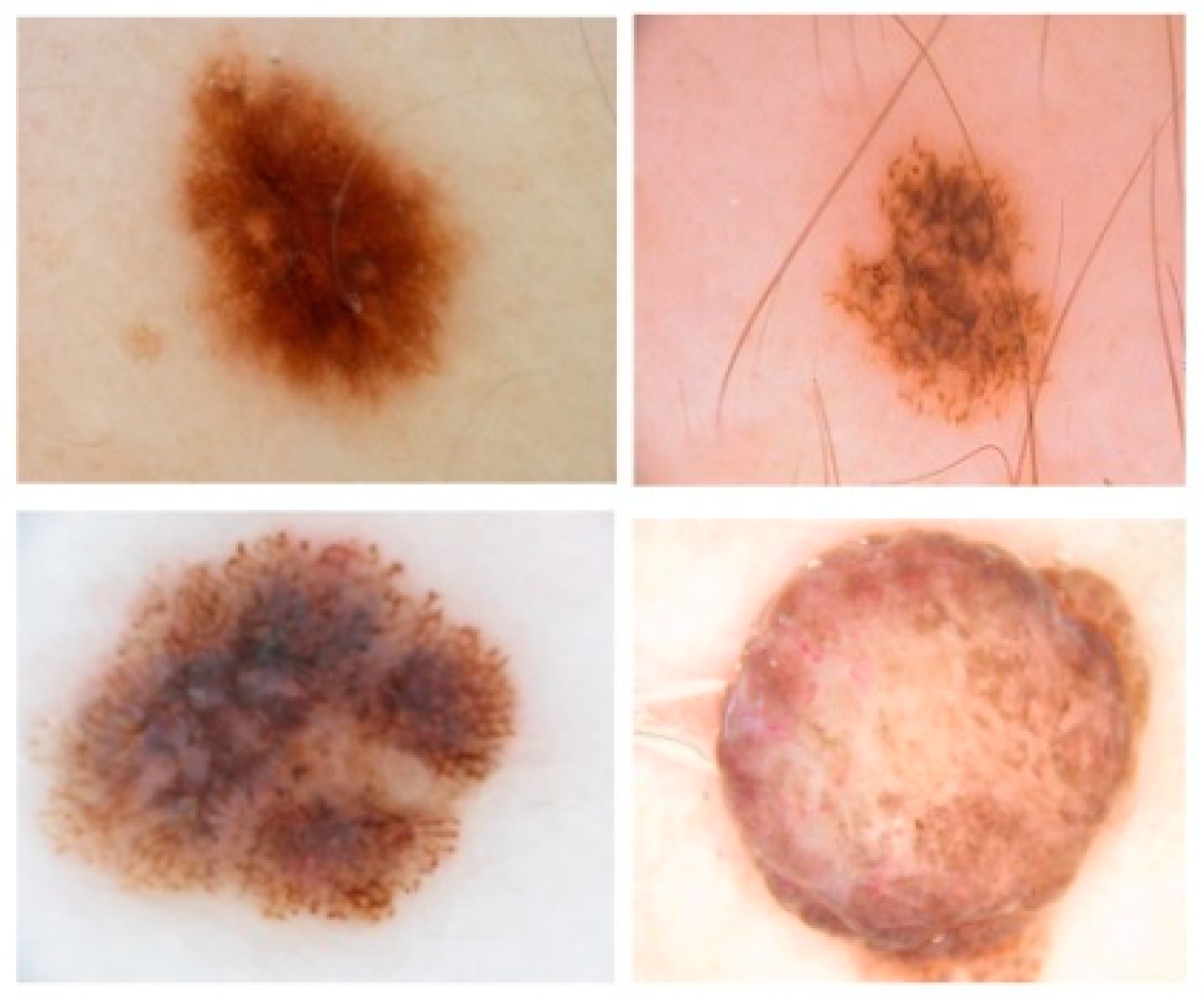
Figure 1. Sample dermoscopic images of skin lesions.
Applsci 10 03658 g001
Figure 2. Dropout neural network. (a) A traditional network with two hidden layers; (b) An instance of a thinned network. Crossed nodes have been dropped.
Applsci 10 03658 g002
Figure 3. Proposed system flowchart.
Applsci 10 03658 g003
Figure 4. Proposed fully convolutional model for skin-lesion segmentation.
Applsci 10 03658 g004
Figure 5. Schematic illustrating an artifact caused by the transposed convolution: (a) checkerboard problem caused by applying a transpose convolution; (b) uneven overlap (with the parameters of stride 2 and size 3).
Applsci 10 03658 g005
Figure 6. Example of bilinear interpolation.
Applsci 10 03658 g006
Figure 7. (a) Rectified linear unit (ReLU) activation function; (b) Derivative of ReLU.
Applsci 10 03658 g007
Figure 8. (a) Parametric ReLU (PReLU) activation function; (b) Derivative of the PReLU.
Applsci 10 03658 g008
Figure 9. True positive, false positive and false negative. Here, the purple square is the ground truth and the black square represents the detected region.
Applsci 10 03658 g009
Figure 10. Sample results of segmented skin lesion: (a) original image (black line is the ground truth); (b) ground truth; (c) result of U-Net; (d) result of FC€1; (e) result of FCN-2; and (f) result of proposed model. Notes: 1. White section in the binary image is the segmented skin lesion; 2. Red lines are the ground truth of the input image.
Applsci 10 03658 g010
Figure 11. Comparing learning curves per epoch.
Applsci 10 03658 g011
Figure 12. The effect of dropout on the learning curve: (a) learning curve with dropout and (b) learning curve without dropout.
Applsci 10 03658 g012
Figure 13. High and low dice coefficient examples (above-given images are original images in validation set). High dice coefficients: (a) 98.26%, (b) 98.87% and (c) 97.74%. Low dice coefficients: (d) 68.41%, (e) 64.97% and (f) 71.58%.
Applsci 10 03658 g013
Table 1. Test accuracy of various U-Net models.
ModelPixel AccuracyDiceIoU
U-Net91.12%78.23%39.26%
FCN-190.47%81.85%40.51%
FCN-291.34%83.26%41.84%
Proposed method94.36%88.33%44.05%
Here: U-Net—original U-Net architecture; FCN-1—U-Net with the PReLU and transpose convolution; FCN-2—U-Net with the PreLU and bilinear interpolation; Proposed method: U-Net with the PreLU, bilinear interpolation and dropout.