1. Introduction
Tidal flats are intertidal, soft sediment habitats, found between mean higher high water (MHHW) and mean lower low water (MLLW) lines [
1,
2] and are present at various locations around the world. Tidal flats are an important part of the coastal zone and play an important role in improving coastal protection, increasing potential land resources, and conserving biodiversity [
3,
4]. The monitoring of tidal flats has great importance for morphological evolution, sediment transformation, and hydrodynamic research [
5]. Therefore, in order to understand the dynamic changes of intertidal areas, topographic monitoring provides the most objective and foundational bases. However, this topographic information remains limited in most coastal areas [
6].
A tidal flat is a “difficult area” to recognize by traditional measurements, such as ground or shipboard surveys, that have high precision (centimeter level) [
7]. Additionally, complete surveys and regular maintenance of updated digital elevation models (DEM) are costly and time-consuming. Data gaps are in the intertidal zone according to most global DEMs products due to the water-impermeable nature of existing remote sensing approaches (e.g., radar used for WorldDEM
TM and Shuttle Radar Topography Mission DEM, and optical stereo-pairs used for ASTER Global Digital Elevation Map Version 2) [
8]. Airborne survey (e.g., light detection and ranging (LIDAR) and radar interferometry (InSAR)) used in land surveying usually have relatively high resolution (0.5–1 m) [
9]. Due to the high-cost to cover a large area and the favourable tidal conditions when flying overhead, Airborne survey methods are also not effective ways to obtain topographic data for tidal flats [
10,
11]. From multiple images obtained over a range of tidal conditions, a set of heighted waterlines can be assembled in the intertidal zone, and from this a gridded DEM can be interpolated [
12,
13]. According to the previous studies, DEMs of intertidal areas had been constructed around the world using waterline method. A DEM having a spatial resolution of 50 m and height accuracy of about 40 cm was formed using the waterline technique applied to satellite Synthetic Aperture Radar (SAR) images from 1991–1994 in Morecambe Bay, U.K [
12]. Ryu et al. (2008) succeeded in generating DEMs with an accuracy of 10.9 cm for the years 1991 and 2000 in the tidal flats of Gomso Bay, Korea [
10]. Tong et al. (2020) applied the waterline method in the Gulf of Tonkin, Vietnam for multi-temporal satellite images to build DEMs with the vertical accuracy of 0.144 m ± 0.05 m in 1989, 2000, and 2014 [
6]. The Yangtze River mouth was also selected as the case example to test the suitability of the approach, and the maximum error for each time slice occurred under lower tide condition (elevation < 100 cm, i.e., 56 cm in 1987, 25 cm in 1993, and 76 cm in 2004) [
14]. In Jiangsu coast, Liu et al. (2012) generated a DEM which contained the error within 47 cm over a large offshore sandbank Dongsha integrating the conventional waterline method with a hydraulic model and multitemporal satellite images [
15]. Kang et al. (2017) explored an iterative waterline method to construct a DEM covering an area of approximately 1900 km
2 of tidal flats in the Radial Sand Ridges (RSRs) and the height accuracy (root mean square error) was 0.182 m [
13].
To construct a DEM, the waterline method usually requires specific conditions. The most important of all is sufficient and high-quality remote sensing images at various tidal levels. In the process of DEM construction, more multi-images should be collected in a shorter time (e.g., a single month or season) so that the change of topography can be neglected. However, limited by weather or image quality, this collection is difficult to achieve in practice. In previous studies, the time span of images was half a year, at least, extending up to 3–4 years [
16]. In addition, the area of tidal flats should be small and stable so that the waterlines can be identified as contour lines with the same tidal level [
17]. Above all, the previous studies mostly manipulated the waterline method in stable areas such as bay or gulf, with relatively homogeneous coastal environments and the vertical error was within 0.5 m [
15]. However, caused by tides, waves, and tidal channel migration, tidal flats are usually faced with high morphological changes [
18]. Just like a large sandbank Tiaozini in RSRs, Jiangsu coast, China, significant temporal and spatial morphological changes occur in tidal flats due to the continual migration of tidal creeks, which can reach several kilometers in two or three months [
3]. According to those variable areas, whether the waterline method can be used to monitoring the topography timely and without interruption needs to be further explored.
Our study attempted to apply the waterline method to an area with high morphological changes and broader regions. To solve this problem, in this study, single images under a low tidal level that can present instantaneous geomorphic distribution are used to construct the DEM. This can help to increase monitoring frequency, and is more suitable to changeable areas. Thus, except for water-edges, we sought to excavate more information (spectral bands, geographic type, and position and distance) from single remote sensing images of tidal flats. These data are used to build a relationship model with measured elevation data. Due to a lack of measured data, the elevation data was collected based on the topography map results in the literature [
13]. Another problem, however, in dealing with elevation data in the context of prediction model development lying in their inherently fuzzy and non-linear relationships with remote sensing data [
19]. To overcome this obstacle, we used an artificial neural network (ANN) as our modelling framework. ANN imitates the information transfer process used by human beings and is applicable to solving complex and nonlinear problems [
20]. There are many types of learning algorithms used to train ANNs, and the back propagation (BP) algorithm is one of the most commonly used techniques in the field [
21]. It has the advantages of a nonlinear, sample-based, free model structure [
22], and has been used to correlate large and complex datasets without any prior knowledge of the relationships between them in many disciplines, such as in water depth retrieval [
23,
24,
25]. However, owing to shallow water restrictions or high water turbidity, few studies have applied a BP ANN model to simulate the topography of large-scale tidal flats.
The objective of this study was to construct a DEM of an intertidal zone with high geomorphic evolution. Based on the resulting map of the waterline method, an ANN model using a suite of geomorphological factors from a single remote sensing image was developed and evaluated. Taking the Tiaozini tidal flats in the Central Jiangsu coast as the study area, with the support of remote sensing (RS), geographic information system (GIS), and neural network simulation technologies, DEMs for remote sensing images taken at other times were obtained. The accuracy and applicable conditions for constructing DEMs of tidal flats were also be discussed.
2. Study Area and Materials
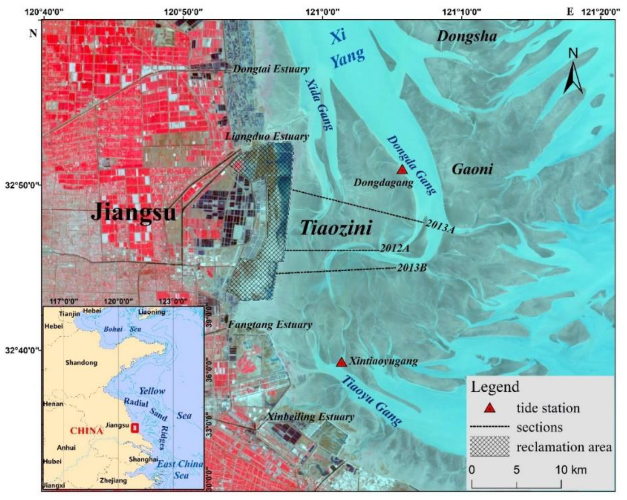
The large (about 500 km
2) Tiaozini tidal flats are located in the core intertidal area of the Radial Sand Ridges (RSRs) of the Jiangsu coast, China. The widths of the tidal flats here are about 14–20 km, and the slope is only 5‰–10‰ [
3]. The RSRs are controlled by a large-scale tidal wave system that is determined by the land boundaries of China and the Korean Peninsula. The tidal wave first enters the Southern Yellow Sea, and part of the wave is reflected by the Shandong Peninsula, forming an anticlockwise rotational tidal wave system. The rotational wave meets the following progressive wave from the southern Yellow Sea, resulting in the formation of large-scale fan-shaped sand ridges [
26]. The tidal water from both north and south meet in Tiaozini every day, forming the largest tidal range. The maximum tidal range (9.39 m) was observed for the south channel Tiaoyugang in Tiaozini [
27]. Due to such a complex hydrodynamic environment, these tidal creeks (Xidagang, Dongdagang, and Tiaoyugang in
Figure 1) swing violently [
28,
29]. Based on a comparison of the before-and-after remote sensing images, the amplitude can reach 3~5 km over half a year. The tidal creek migration inevitably leads to geomorphic changes. In addition, the reclamation activity in this area (completed for 67 km
2 (
Figure 1)) inevitably exerts a profound impact on the surrounding environment, such as the geomorphology, the dynamic conditions, sediment transport mechanisms, biotic habitat, etc. [
4]. In order to effectively assess and support the impact of reclamation activities, the topographic monitoring of tidal flats is urgently needed.
This study collected 18 HJ-1A/B charge coupled device (CCD) images and three Landsat images acquired at different tidal stages from 31 December 2013 to 28 May 2014 [
13]. These images were used to construct the initial DEM via the waterline method. The remote sensing images are HJ-1 CCD data that have a nadir pixel resolution of 30 m, a width of view of 360 km, and a temporal resolution of two days [
30]. Four bands are B1 (0.43–0.52 μm), B2 (0.52–0.60 μm) and B3 (0.63–0.69 μm), and B4 (0.76–0.90 μm). In particular, the 21 March 2014 HJ-1 image (
Table 1) under the lower tidal conditions and Tiaozini’s initial DEM acquired by the waterline method were input into an ANN simulation model as training data. Two other images (11 February 2012 and 11 July 2013) (
Table 1) were applied as test data for the ANN model to simulate the corresponding DEMs at the same time. All the HJ-1 images are clear under good atmospheric conditions. A topographic map (1:50,000) of the Jiangsu coastal zone was collected for geometric rectification of these HJ-1 satellite images. The correct accuracy was controlled within a pixel. A QUAC (QUick Atmospheric Correction) [
31] of the HJ-1 images was also carried out in this study. This method provides the automated atmospheric correction of the reflective spectral region (0.4~2.5 μm) in the ENvironment for Visualizing Images (ENVI) software (Exelis Visual Information Solutions, Inc., Boulder, CO, USA) and creates an image of the retrieved surface reflectance, scaled into two-byte signed integers using a reflectance scale factor of 10,000. QUAC was carried out in the ENVI software Toolbox using the following steps: QUAC initiation, radiometric correction, atmospheric correction, and quick atmospheric correction. Two real-time tide stations (Dongdagang and Xintiaoyugang) were established around the north and south sides (
Figure 1). The tidal level data were applied to the assignment of these waterlines. Three measuring sections in February 2012 and July 2013 were collected to evaluate the accuracy of the DEMs simulated by the ANN model. The Chinese National Height Datum 1985 (CNHD 1985) was adopted for the tide stations, sections, and DEMs. The coordinate system was WGS_1984_UTM_Zone_51N in ArcGIS software.
3. Methods
The method can be divided into the following steps:
Training data (output side) preparation of ANN model. The output side was the elevation of the tidal flats. Due to a lack of measured data, a result map from a previous study based on the waterline method was used as the output side of the training data. Thus, a topographic map of the Tiaozini tidal flats was obtained using remote sensing images over half a year (31 December 2013 to 28 May 2014 in
Table 1) according to the literature [
13].
Training data (input side) preparation of the ANN model. The input side has seven parameters in three categories (multi-spectral bands, geographical coordinates, the distance from waterlines) which were exacted from the HJ-1 image of 21 March 2014 under the lower tidal level.
Model design. Based on training data, the “7-15-15-1” double hidden layers with optimized training structures were confirmed via continuous training and comparisons.
Model simulation and precision evaluation. The elevation estimations obtained for the testing and training datasets based on the HJ-1 image (21 March 2014) were compared to the initial DEM obtained by the waterline method. After geometric correction and histogram matching, the input parameters were extracted from the two HJ-1 images (11 February 2012 and 11 July 2013), input into the ANN model, and used to output the estimated elevation. The height accuracy of the two DEMs was evaluated based on three transects of the in situ measured data.
3.1. Topographic Mapping of Tidal Flats by the Waterline Method
The waterline method, which is currently considered to be the most useful approach [
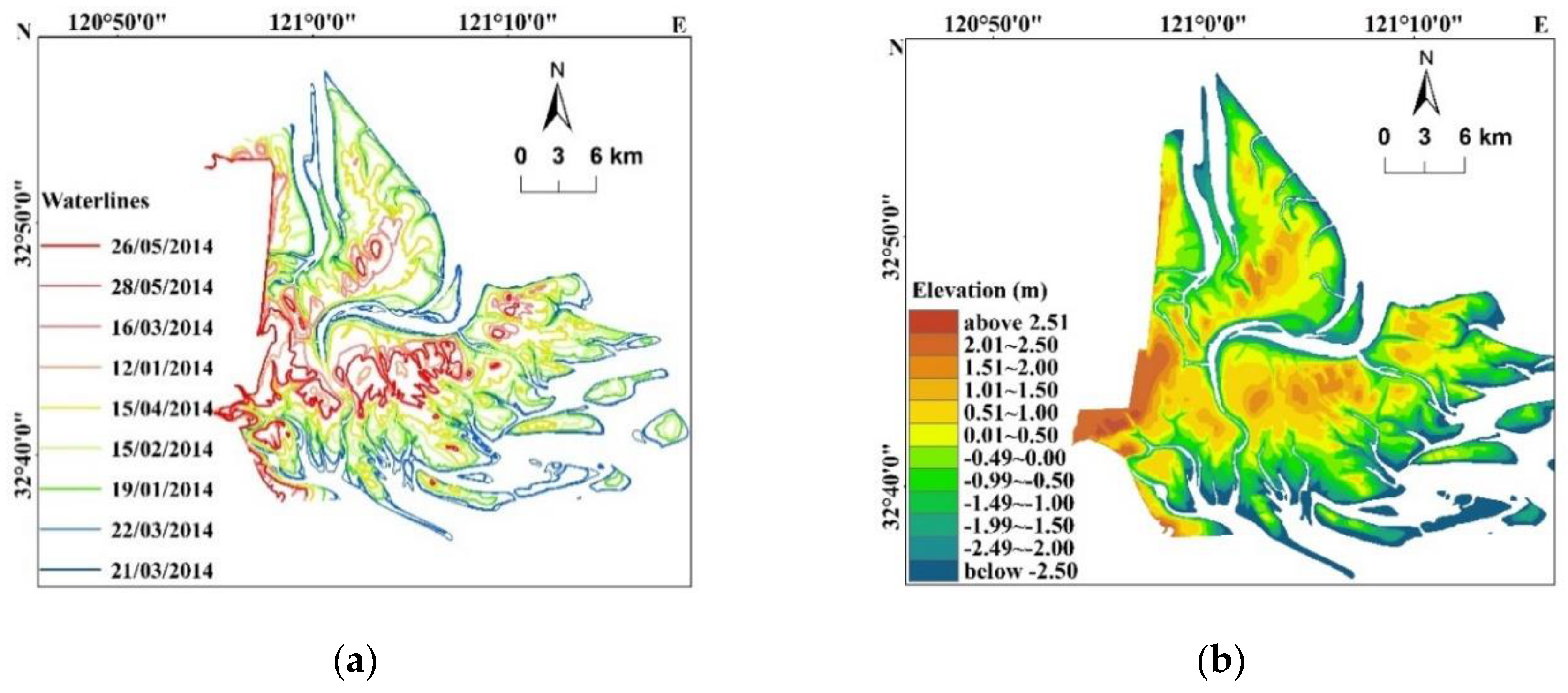
12], makes use of the ever-shifting boundary between tidal flats and adjacent water areas, whose positions can be regarded as a quasi-contour line of the topography (not a true contour line because the water level of the tidal wave varies horizontally). The waterline method has been previously applied to the Jiangsu coast. In this study, 21 waterlines were extracted from remote sensing images (partly listed in
Figure 2a). Then, based on a 2D hydrodynamic model, the waterlines were given elevation values. The DEM was constructed by the interpolation method using these heightened waterlines (
Figure 2b). More details can be found in the work of Kang et al. (2017) [
13].
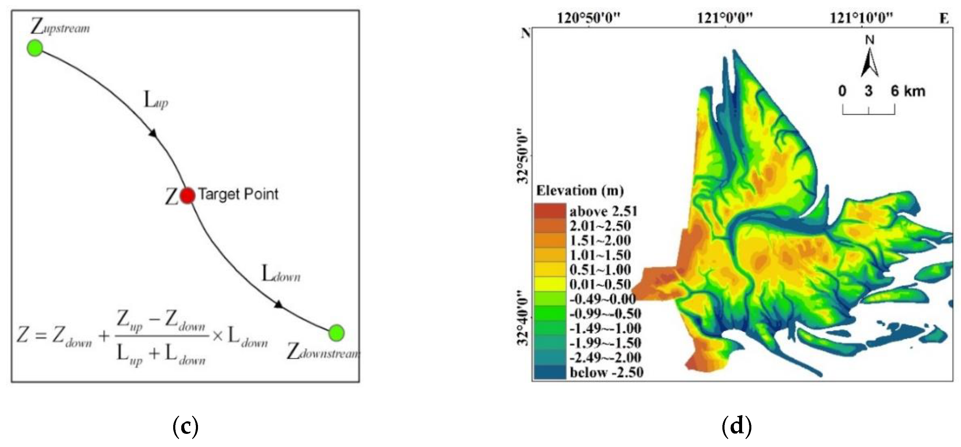
The tidal creeks, however, lack data. Thus, in this study, in order to gain seamless DEM data, we interpolate the topographic data using the linear method. A previous study [
32] showed that along a tidal creek, the elevation presents a linear attenuation from its head to its mouth. Firstly, the center lines of the tidal creeks were extracted based on the waterline and remote sensing image from head to mouth (that is, from upstream to downstream along one creek). Secondly, the centerline was given an elevation value by using the linear interpretation method as shown in
Figure 2c. The elevation of the head (
Zupstream) was the height value of the lowest waterline, and that of the mouth (
Zdownstream) was set in advance based on known survey sections and charts. The middle points (
ZTarget) along the centerline of the tidal creek were calculated based on the linear interpolation formula shown in
Figure 2c. Lastly, we added the centerline with height information, and the seamless DEM shown in
Figure 2d was generated by Natural Neighbor spatial interpolation using ArcGIS software. This DEM will be used as training data in the output layer of the ANN model in the next section.
3.2. Input Factor Extraction from Remote Sensing Images
In this study, seven parameters in three categories extracted from remote sensing images were selected as the nodes of the input layer of the ANN model: (1) multi-spectral bands (HJ-1: B1, B2, B3, B4); (2) geographical coordinates (X, Y); and (3) the distance from waterlines (D).
Remote sensing spectral bands: The intertidal zone can be separated into three distinct zones related to elevation and tidal level. The lower tidal flats lie between the mean low water neap and the mean low water spring tide levels and are often subjected to strong tidal currents, the middle flats are located between the mean low water neaps and the mean high water neaps, and the upper flats lie between the mean high water neap and the mean high water springs. Different zones have different spectral characteristics. At upper tidal flats, the reflectance in the NIR range (B4: near-infrared, 0.76–0.90 μm) tends to be higher and the B3 (red, 0.63–0.69 μm) tends to be lower due to a small amount of vegetation and lower water content. The B1 (blue, 0.43–0.52 μm) and B2 (green, 0.52–0.60 μm) can be used to interpret and identify tidal channel and creeks in the lower tidal flats due to relatively high reflectance. However, there is great diversity in the morphology, sediments, bedforms, and ecology of these three zones that relates to the changing balance of physical, sedimentological, and biological forces. These diversities are inevitable reactions through all (HJ-1: four) spectral bands of satellite images. Only dependking on a single band and simple linear statistics cannot establish an accurate association with elevation of tidal flats. Thus, in this study, four bands were all considered as elevation-related elements in the ANN model with nonlinear method. The images are different in different moments in the same tidal flat due to the weather and atmospheric conditions. Thus, the preprocessing of images is required. In this paper, we used geometric correction and histogram matching for this preprocessing. Histogram matching is a mathematical transformation used to eliminate and correct the color and brightness differences between the two images. The histogram matching process is done based on ERDAS 9.1 software (Main, Image Interpreter, Radiometric Enhancement, and Histogram Matching).
Geographic coordinates: The spatial stability of the tidal flats can be represented by basic geographical coordinates. For the same area, topographic data often change within a certain range, while the high value and low value of elevation remain in a controllable interval. In this study, geographic coordinates were used as the input factors to provide the range of elevation in the simulated tidal flats. All coordinates are located in the WGS_1984_UTM_Zone_51N datum.
Distance from waterlines: In the Tiaozini tidal flats, tidal creeks like Xidagang, Dongdagang, and Tiaoyugang (
Figure 1) play a core role in geomorphic evolution. These flats are considered as positive topography ‘+’, while the creeks are a type of negative topography ‘-’. For the flats, the longer the distance from the waterline, the higher the elevation, and vice versa; for the creeks, the longer the distance from the waterline, the lower the elevation, and vice versa. Hence, the distance D is considered an important factor in topographic modelling. Based on the waterline, the area was divided into two categories: flats ‘+’ and creeks ‘−’. According to each pixel, the D has a positive or a negative value. Secondly, based on the ArcGIS spatial analysis, the shortest distance (D) between each pixel and waterline is calculated. The D factor is a vector feature that contains not only the distance length but also positive and negative attributes.
3.3. Model Design
Artificial neural networks (ANNs), as statistical learning models, are a research focus in image processing and the remote sensing retrieval of parameters on the Earth’s surface based on remote sensing images. The water depths of remote sensing models based on ANN have found a wide range of applications around the world [
22,
24]. Atkinson and Tatnall [
21] noted three advantages of ANNs in the remote sensing inversion model. ANNs are more accurate and efficient than other forms of linear statistics, especially for very complex feature spaces or multi-source data with different statistical distributions; ANNs allow prior knowledge (e.g., a geomorphology value) to be used as an input to build the model; and ANNs can couple different types of data, facilitating collaborative research. Therefore, theoretically, an ANN is an effective method to simulate the elevation of tidal flats based on remote sensing images.
A multi-layer feed-forward back propagation network was proposed by Rumelhart [
33] and is widely used for data prediction. The mechanism is that the weights and thresholds of the network were modified to minimize the error between the real and simulated values. The basic BP algorithm includes two processes: forward propagation of the signal and backward propagation of the error. That is, the error output is calculated in the direction from input to output, and the adjustment weights and thresholds are performed in the direction from output to input. During forward propagation, the input signal acts on the output node through the hidden layer and undergoes a nonlinear transformation to produce the output signal. If the actual output does not match the expected output, the error is transferred back to the reverse propagation process. After repeated learning and training, the network parameters (weights and thresholds) corresponding to the minimum error are determined.
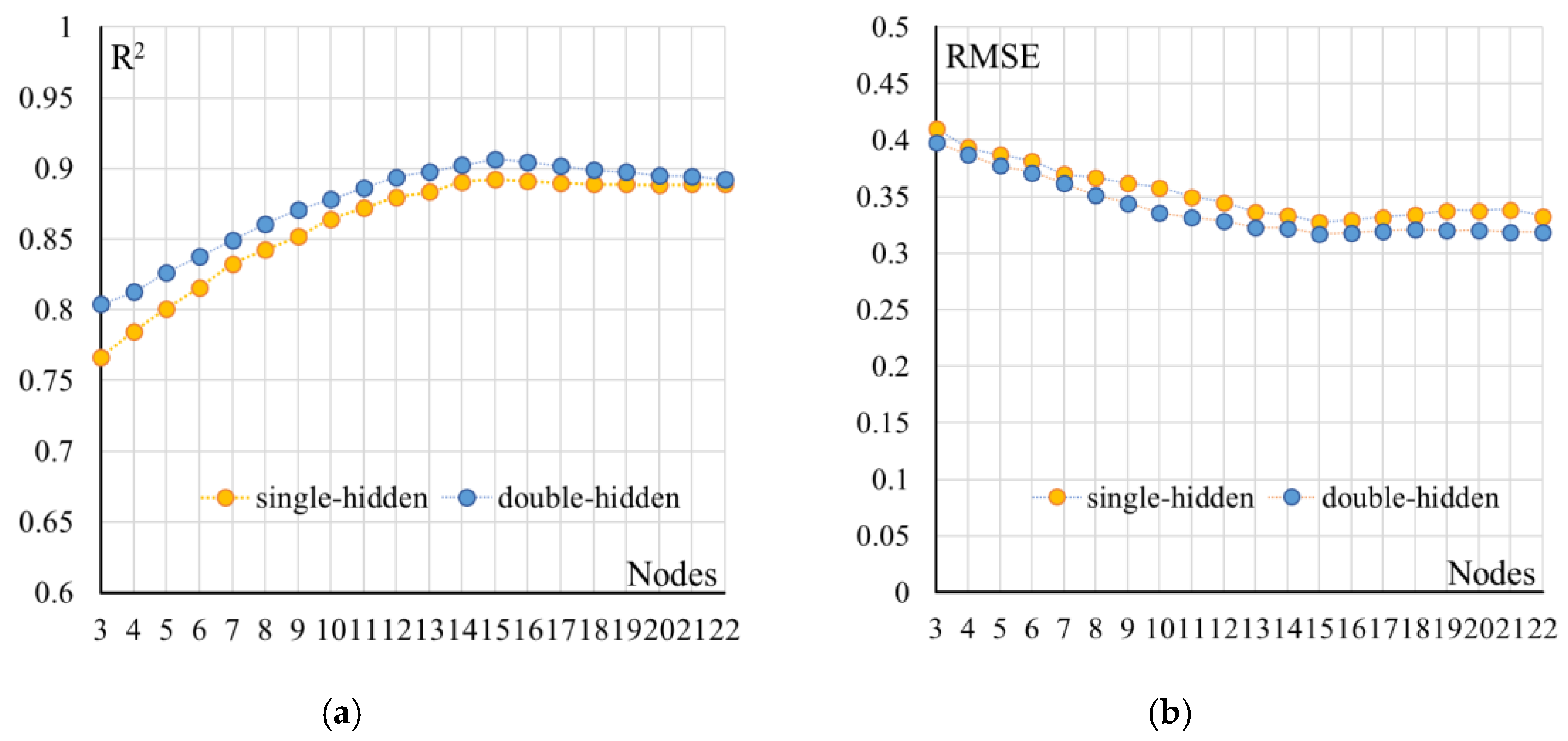
Designing the structure of a BP neural network model, however, is still a problem. BP neural networks with at least one hidden layer are necessary for arbitrary nonlinear function approximation. In practice, one or two hidden layers (that is, three layers or four layers including the input and output layers) are commonly used. In this study, the DEM (
Figure 2d) generated in the previous section is considered as the expected output vector. Using the HJ-1 spectral bands (B1, B2, B3, B4), the geographical coordinates (X, Y), and the distance to the waterline (D), a total of seven vectors were prepared as the input layer. Taking the HJ-1 image of 21 March 2014 as the input, single-hidden, and double-hidden layers with nodes (from 3 to 22) for each layer network were developed. The root mean square error (RMSE in Equation (1)) and coefficient of determination (R
2 in Equation (2)) were used as evaluation indices to select the optimal model structure. The RMSE shows the dispersion of the sample and reflects the degree of deviation from the true value of the simulation data. R
2 reflects the degree of correlation between the two sets of data. Therefore, when the RMSE is smaller, the R
2 is larger, and the structure is better. The results in
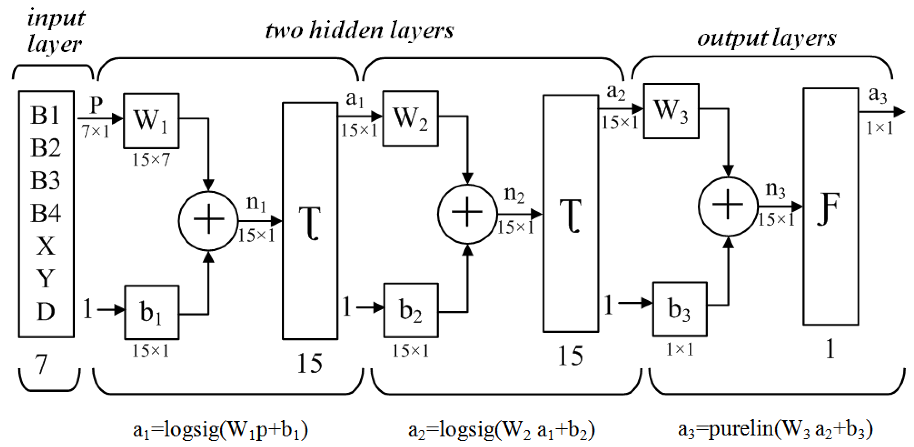
Figure 3 show that the double-hidden layer network is obviously better than the single-hidden layer network. A model with double-hidden layers with 15 nodes per layer model was chosen. The topology of the BP neural network with double-hidden layers is shown in
Figure 4.
3.4. Applications and Preprocessing
Using the variable Tiaozini tidal flats as an example, based on the DEM using the waterline method and the HJ-1 image (21 March 2014), a BP neural network model was constructed (
Figure 5). The input layer of this model has seven node parameters in three categories: reflectance (B1, B2, B3, B4), geographic coordinates (X, Y), and distance (D) from the waterlines. The structure of the ANN model includes double-hidden layers with 15 nodes in each layer. Seven-hundred points evenly distributed in the Tiaozini area were selected and separated into two parts as a training (600) and testing (100) dataset. To determine the network architecture (7-15-15-1), model training and testing were conducted until an acceptable error was reached. This model was also applied to simulate the topography for two other dates based on the HJ-1 images (11 February 2012 and 11 July 2013). The measured data were used to verify the accuracy of the ANN model. A flowchart illustrating the methodology used in this study is shown in
Figure 5.
3.5. Model Assessment and Validation
The results of this study are presented in a digital form of DEMs, and the accuracy of the simulation results is analyzed through measured data. The elevation estimations obtained for the testing and training datasets based on the HJ-1 image (21 March 2014) were compared to the initial DEM (
Figure 2d) obtained by the waterline method. In order to further verify the accuracy of the model application, three measuring sections in July 2013 and February 2012 were collected to evaluate the accuracy of the result according DEMs.
Check points in a grid form were picked out in advance according to the in-site data. Compare the elevation of these points with the actual measured data one by one to get the error of each point, and then calculate the RMSE (Equation (1)) and R2 (Equation (2)). In addition, the error distribution chart can also assist in the analysis of model assessment and validation. Comparative maps between the simulated and measured data can show the accuracy of the results more intuitively. Additionally, the frequency histogram of the residuals can elaborate the distribution range and characteristics of error directly. Accuracy validation was carried out and showed in the next paragraph.
4. Results
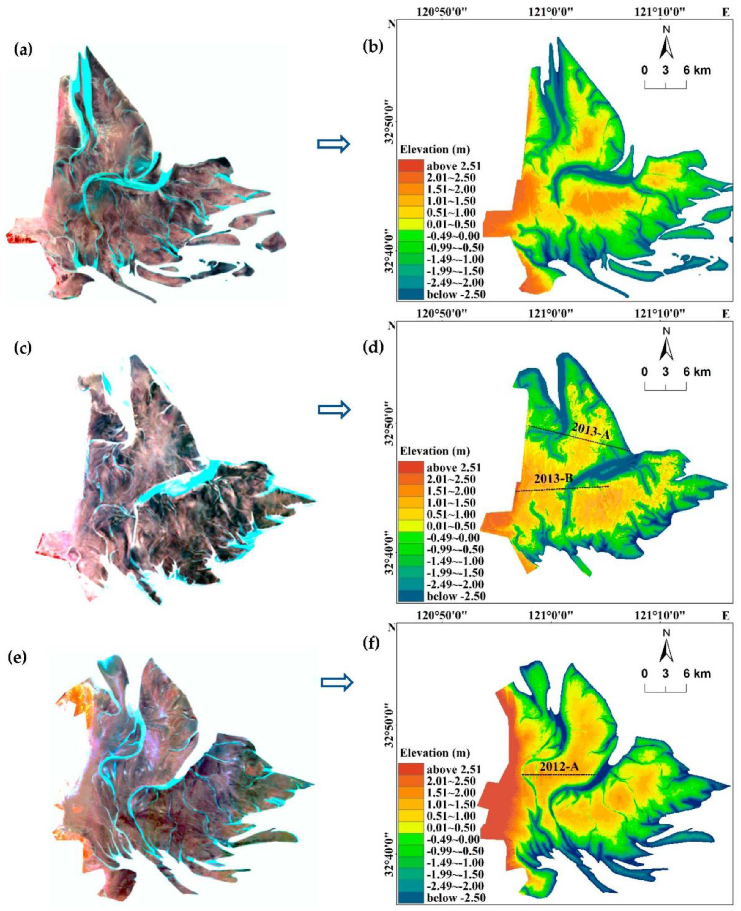
Based on the images from 21 March 2014 (
Figure 6a), the trained models were run to test the dataset. The elevation estimations obtained for the testing and training datasets based on the HJ-1 image (21 March 2014) were compared to the DEM data by the waterline method.
Figure 6b shows the simulated topography map for 21 March 2014. After geometric correction and histogram matching, the input parameters were extracted from the two HJ-1 images (11 July 2013 and 11 February 2012) (
Figure 6c,e), input into the ANN model, and used to output the estimated elevation. These types of estimates are used to interpolate a contour map or generate a digital elevation model. Two fresh DEMs (11 July 2013; 11 February 2012) were obtained and are shown in
Figure 6d,f. The resulting maps were provided with 30 m precision to facilitate this comparison according to the spatial resolution of HJ-1 image.
As shown in
Figure 6, the resulting DEMs are consistent with the instantaneous situation of the remote sensing images. There are some similarities and differences. On the one hand, the similarities are the trend of macro-morphology. In the Tiaozini tidal flats, the west near the land are higher than those in the east near the sea. Additionally, the elevation of the tidal flats is higher than the tidal creeks. On the other hand, the three DEMs are obviously different due to the variable tidal creeks. Tiaozini is mainly affected by the comprehensive influence of the three major tidal creeks of Xidagang, Dongdagang and Tiaoyugang (
Figure 1). Due to the different hydrodynamic strength between the north and the south, the tidal creeks of Xidagang and Dongdagang oscillates very frequently, resulting in topography changes are very rapid. That is why the topography of the three DEMs looks different. The remote sensing image provides planar information that can directly display the two-dimensional shape of the Tiaozini tidal flats. Through the model of this study, the elevation information is added and help to convert from two-dimensional image to three-dimensional topography.
As shown in
Figure 7, 700 points evenly distributed in the Tiaozini area were selected and separated into two parts as a training (600) and testing (100) dataset. The trained models were run to test the dataset. The elevation estimations obtained for the testing and training datasets based on the HJ-1 image (21 March 2014) were compared to the initial DEM (
Figure 2d) obtained by the waterline method. As shown in
Figure 7a,b, the training dataset and testing dataset comparison map showed good correlation. The R
2 of the training dataset was 0.90, and the R
2 of the testing dataset was 0.91. The root mean square error (RSME) of the training dataset was 0.33 m, and the RSME of the testing dataset was 0.31 m. The error value of the training data was 21% within ± 0.1 m, 51% within ± 0.3 m, and 71% within ± 0.5 m. The error value of the test data was 18% within ± 0.1 m, 55% within ± 0.3 m, and 76% within ± 0.5 m.
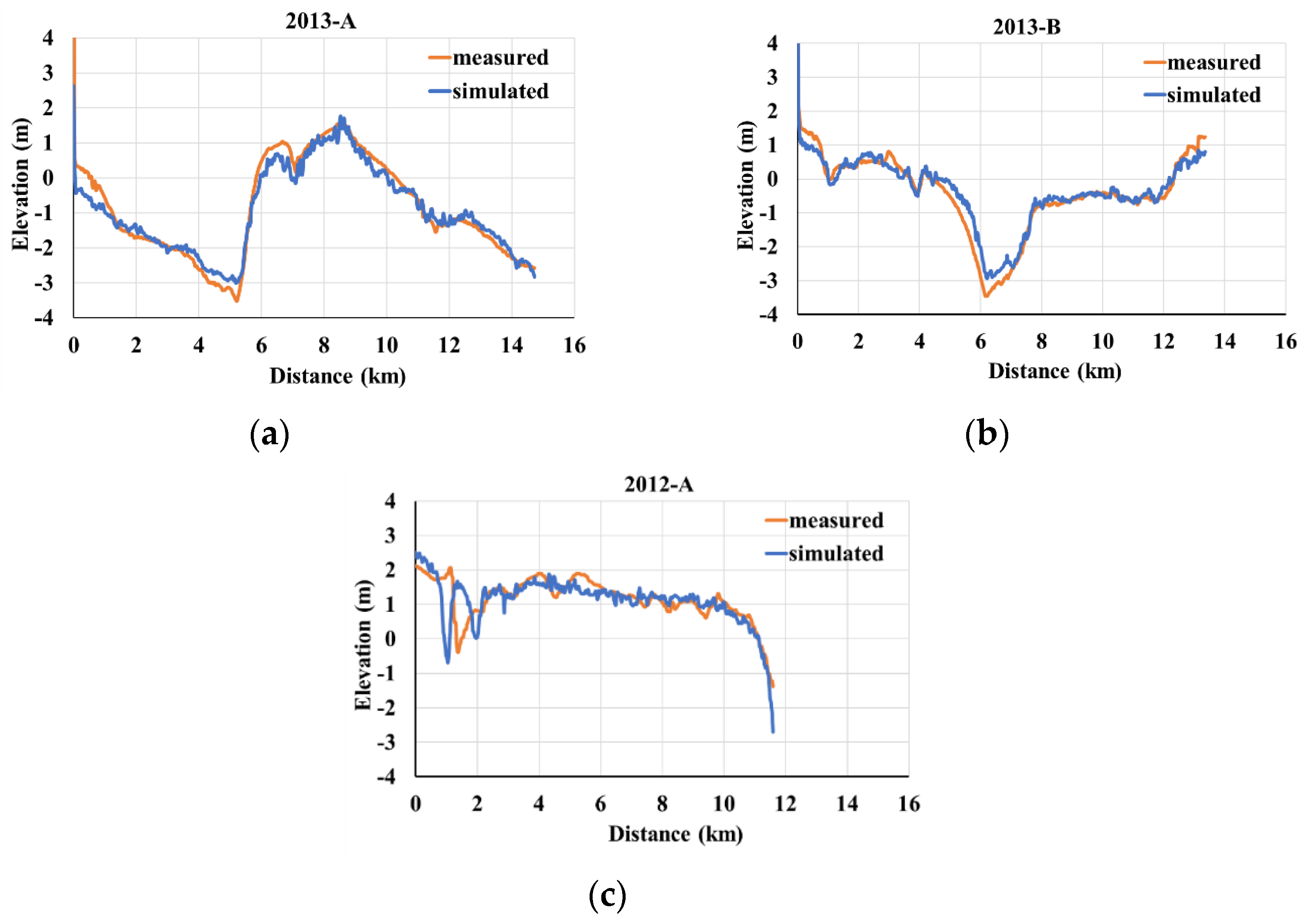
As shown in
Figure 8, the three measured sections in 2012 and 2013 shown in
Figure 8b,c were used to compare the simulated DEMs. The agreement between the cross-sections and the measured data was good, especially in the case where all three cross-sections pass through two big tidal creeks (Xidagang, Dongdagang in
Figure 1). The 15 km long comparison curve of the 2013-A section (
Figure 8a) crossed the Xidagang tidal creek. The accuracy was calculated by measuring points every 30 m; the RSME was 0.32 m, and the R
2 was 0.90. The accuracy of the 13 km long 2013-B section (
Figure 8b) crossing the Dongdagang tidal creek was calculated by measuring points every 30 m; the RSME was 0.26 m, and the R
2 was 0.91. The 11 km long 2012-A section (
Figure 8c) was distributed on the tidal flats between Xidagang and Dongdagang. The RSME of 2012-A was 0.39 m, and the R
2 was 0.85. Based on the comparison curve of the sections in
Figure 8, the error is larger near the creeks and smaller on the flats area. In Radial sand ridges area, intertidal flats are typically dozens of kilometers wide with an average slope of approximately 0.2%, and an increase in slope to 1.5% near the tidal creeks [
15]. In the vicinity of the waterline, the error tends to increase due to the steep change in slope.
From the above, the overall distribution of the geomorphic trends can be accurately simulated to display a detailed representation of the topography. The resulting DEMs are consistent with the instantaneous situation of the remote sensing images. According to the ANN model, the training dataset and testing dataset comparison map showed good correlation based on the images from 21 March 2014. The comparison of three cross-sections which pass through two big tidal creeks showed a good correlation between the simulated DEM and in situ data. The spatial resolution of the simulated DEM can reach 30 m according to the HJ-1 image, and the RSME accuracy was about 0.3–0.4 m. This ANN model can be used for monitoring the varied tidal flats area.
5. Discussion
Taking Tiaozini as an example, a combined method (waterline method and ANN model) was designed to estimate the elevation of changeable tidal flats. The waterline method was elaborated in detail according to the published literature [
13] and applied to support the initial training data for the ANN model. A feed-forward neural network using the back-propagation training algorithm was constructed to simulate the elevation of tidal flats in this study. On the one hand, from the perspective of input parameters, different combinations that affect the accuracy of DEM results were discussed. On the other hand, based on previous studies, a discussion was carried out in terms of vertical accuracy, horizontal accuracy, and time accuracy of the DEM results in different tidal flats sites.
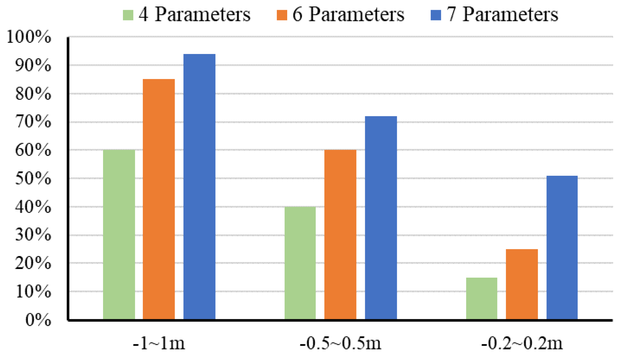
According to this ANN model, input parameters are crucial for simulation accuracy. In this study, three different combinations of input parameters were discussed. The first one is only four input nodes (B1, B2, B3, B4), and the network structure of ‘4-15-15-1′. The second one is six input nodes (B1, B2, B3, B4, X, Y), and the network structure of ‘6-15-15-1′. The last one is seven input nodes (B1, B2, B3, B4, X, Y, D), and the network structure of ‘7-15-15-1′. We used the same input data from the image (21 March 2014) to simulate the topography and compared the accuracy of three ANN models with different network structures. The seven-parameter group had the smallest error compared to the six-parameter and four-parameter groups. The RMSE can reach 0.32 m, and the R
2 can reach 0.90 (
Table 2).
Figure 9 shows the distribution of the error percentage. Only 60% of the error value of the neural network model based on four parameters was within ± 1 m, 40% was within ± 0.5 m, and 15% was within ± 0.2 m. With the addition of parameters, the accuracy improved rapidly. The error value of the six-parameter model was 85% within ± 1 m, 60% within ± 0.5 m, and 25% within ± 0.2 m. The error value of the seven-parameter model was 94% within ± 1 m, 72% within ± 0.5 m, and 51% within ± 0.2 m. This result shows that parameter D contributed the most to improving accuracy. In addition, each tidal creek system occupies a “drainage basin” on the tidal flat [
3]. The topographical changes are largely related to the tidal creeks, which migrate frequently [
29]. During the tide rising, the water flows along the tidal creeks to the flat’s surface. When two water flows from adjacent creeks meet each other at the middle flats, the velocity decreases, and the sand is deposited in this confluence zone. Thus, the elevation is lower near the tidal creeks and higher in the tidal flats and sand ridges. Toward the center of the flats, the elevation value gradually increases with distance, and toward the center of the tidal creeks, the elevation value gradually decreases with distance. Parameter D reveals the basic layout of the topography. In addition, the nonlinear ANN model’s free structure allows us to consider the nonlinear relationships between multiple parameters and elevations, thus allowing more accurate estimations to be obtained. Since the ANN models (a black box model) do not have to consider the factors affecting the reflective properties of water columns and do not have to be trained by newer in-situ measurements, this methodology can be practically applied without handling any complex reflectance separation process and can also be reliably used for repetitive bathymetric mapping, provided that there is an available representative input dataset.
The waterline method is the only current useful approach in the practical application of satellite remote sensing to tidal flat environments [
10,
12]. It has been successfully applied to many intertidal flat zones worldwide according to precious studies. We selected five typical sites (Morecambe Bay, U.K. [
12], Gomso Bay, Korea [
10], Gulf of Tonkin, Vietnam [
6], the Yangtze River mouth [
14], and Dongsha Sandridges [
15]) to compare with Tiaozini in our study in terms of vertical accuracy, horizontal accuracy and time span of DEM results. Details areelaborated in
Table 3.
DEM vertical accuracy: According to the previous studies, the accuracy of DEMs obtained by the waterline method is mostly within 0.5 m. For the more stable area, just like Gomso Bay, Korea, Ryu et al. (2008) succeeded in generating intertidal DEMs with an accuracy of 10.9 cm in the tidal flats [
10]. In [
6], the vertical accuracy reached 0.144 m in the northern coast of Vietnam, which is a stable ground. In Dongsha Sandbank of the Jiangsu coast (relatively unstable area), a DEM effectively contains the average height error within 47 cm [
15]. In the author’s previous study, the accuracy of the DEM obtained was within 0.2 m in Jiangsu’s near shore [
13]. Thus, the stability and complexity of tidal flats often determines the level of accuracy. Mason et al. (2001) indicated that the vertical errors are different at different slopes. On 1:500 slope beaches 18–22 cm is achieved. This rises to 27 cm on 1:100 slope beaches, and 32 cm on 1:30 slope [
34]. As shown in
Table 3, in Tiaozini which is the extremely unstable area, the vertical accuracy can reach between 0.3 m and 0.4 m. It was credible and within reasonable superior range.
DEM horizontal accuracy: Horizontal accuracy is less involved in previous studies Due to the different distribution density and sources of remote sensing images. The waterline method uses medium resolution remote sensing image data to extract the water edge line. Since the waterline itself has an accuracy of one pixel (e.g., 30 m), no matter how many waterlines are located at different tide levels, the DEM horizontal accuracy can only be infinitely close to, but less than one pixel (e.g., 30 m) [
16]. As shown in
Table 3, horizontal accuracy in previous studies was 30–60 m. Our study used each pixel of the remote sensing image to participate in the calculation, allowing the spatial resolution (e.g., 30 m) to be reached. From the perspective of horizontal accuracy, our method is better. However, the simulation results often require smooth fitting to remove noise from the DEM results.
The timeliness of DEM acquisition: Because the waterline method requires a certain time span, it is suitable for relatively stable tidal flat areas, like areas with little or no change within a short time. At present, sufficiently high-quality remote sensing images are the core of the waterline method. In previous studies, the time span of images was one year, at least, up to as much as 3–4 years, as shown in
Table 3. However, areas where the tidal flats change drastically, such as Tiaozini, the tide water from both north and south meet there every day [
3]. Additionally, the topography of tidal flats is highly susceptible to affected changing tidal creeks, just like Xidagang, Dongdagang, Tiaoyugang feature intensive erosion and deposition [
18]. Our model can invert the synchronous topography of the tidal flat at the synchronization time of remote sensing image, which greatly improves its timeliness to monthly levels. From the perspective of time accuracy, our method is better, especially in tidal flat areas with drastic changes. On the time axis, the topographic map is generated by the waterline method for half a year or one year. Within this period, the ANN model can provide assistance for topography monitoring. Through the integrated use of these two methods, we can achieve a long-term observation system that provides continuous DEMs of tidal flats.
The model in this study also has some issues that need to further improve and be verified. Due to a lack of large-area measured data, we used the topographic results via the waterline method as training data for the ANN model. The simulated DEM of the ANN model has relatively good accuracy, which is also reflected by the reliability of the waterline method, and the waterline method’s ability to effectively support ANN simulations. At the same time, the data source of the ANN model was remote sensing image data at a low tide level, which will inevitably affect the input parameters and simulated accuracy. Thus, in addition to selecting low-tide flat images, it is necessary to further explore the influence of the tide level when constructing a topographical simulation model in future studies. In addition, the error was larger in the area of tidal creeks, more measured data should be obtained and input into the model to improve the accuracy around this area.
6. Conclusions
The monitoring of tidal flats has great importance for morphological evolution, wetland protection, and coastal management. Tiaozini, the center tidal flats of the Jiangsu coast, China, changes quickly because of the swing of its tidal creeks. Thus, it is difficult to obtain relevant in situ topographic data. To solve this problem, based on remote sensing images, we constructed an ANN model with a multi-layer feed-forward back propagation algorithm to simulate the elevation of tidal flats. The structure of the ANN model includes double-hidden layers with 15 nodes in each layer. The input layer of this model has seven nodes: reflectance (B1, B2, B3, B4), geographic coordinates (X, Y), and distance (D) from the waterlines. The output layer selects the elevation data obtained from the waterline method in case of insufficient measured data. Based on the three HJ-1 images (21 March 2014; 11 February 2012; 11 July 2013), after the necessary preprocessing, three fresh DEMs were simulated by the ANN model. Through section verification, the vertical accuracy was found to be between 0.3 and 0.4 m, and the horizontal accuracy was able to reach 30 m, which is equal to the spatial resolution of the HJ-1 image. An artificial neural network, with its strong learning and adaptive ability, can be a powerful aid for the waterline method. In this way, especially in tidal flat areas of rapid change, long-term and continuous monitoring can be achieved.


