Article

Numerical Simulation of Vacuum Leak Jet and Jet Noise

1
College of Aerospace Science and Engineering, National University of Defense Technology, Changsha 410073, China
2
China Aerodynamics Research and Development Center, Mianyang 621000, China
3
Beijing Institute of Spacecraft Environment Engineering, Beijing 100094, China
*
Author to whom correspondence should be addressed.
Appl. Sci. 2020, 10(10), 3640; https://doi.org/10.3390/app10103640
Submission received: 20 April 2020 / Revised: 18 May 2020 / Accepted: 22 May 2020 / Published: 25 May 2020
(This article belongs to the Special Issue Modelling, Simulation and Data Analysis in Acoustical Problems Ⅱ)

Abstract

:

Featured Application

Leak mechanics in aerospace applications.

Abstract

With the explosive growth of space debris, collisions among space debris and spacecrafts seem to be inevitable, which may greatly threaten the structure of on-orbit spacecrafts as well as astronauts’ safety. It is of crucial importance to locate the leak source and evaluate the corresponding damage quickly and accurately to ensure the safety of astronauts and spacecraft equipment. It is widely accepted that acoustic emission method can be used to detect on-orbit leak for space station; however, accurate prediction of vacuum leak noise in space station is difficult as jet and jet noise in vacuum environments are different from those in terrestrial environment. Therefore, this paper tries to investigate sound generations of vacuum leak jet by numerically analyzing dynamics of unsteady vacuum jet flow. Specifically, numerical simulation based on realizable k-ε model is adopted to study the aerodynamic properties and the aeroacoustic characteristics. Results show that RANS turbulent model can capture the pressure fluctuation with high computation efficiency and acceptable accuracy. Secondly, leak from 1 atm to vacuum forms a supersonic flow with Mach number ranging from 2 to 3, accompanied by obvious gradients of steady density, pressure, and temperature. However, the terrestrial leak from 2 atm to 1 atm forms subsonic jet flow with gradually varying gradients of density, pressure, and temperature. Thirdly, obvious reflections of pressure perturbations at the surface, with the mean free path of air molecule being 0.6 mm, can be found and form cavity-like acoustic resonance. Such resonant mechanism contributes to harmonic acoustic properties of the vacuum jet noises besides the broadband turbulent mixing noises.

1. Introduction

On April 19, 1971, the world’s first space station, Salyut 1, was successfully launched into orbit, marking the arrival of space age. In the following decades, the U.S. Skylab, the Mir Space Station, and the International Space Station (ISS) were successively built and continuously developed, becoming the base of deep space exploration. However, continuously growing space debris increases collision probability among space debris and spacecrafts, which has caused widespread international concerns [1]. It was reported that many leak accidents occurred on the ISS [2], leading to an urgent demand of on-orbit leak detection. The differential pressure method [3] has been widely used on the pressure vessels of spacecrafts to detect the occurrence of leak. However, it cannot give the leak location. In order to locate the leak-induced noise source, on-orbit sensing technology based on acoustic emission has drawn widespread attention due to its low resource occupancy, little structural constraints and real-time monitoring [4]. In order to verify the effectiveness of the acoustic emission technology, the European Space Agency (ESA) conducted verification tests on the experimental cabin of the ISS [5]. Furthermore, a handheld ultrasonic leak detector developed by National Aeronautics and Space Administration (NASA) has been successfully applied to leak detection in orbit [6].
The current acoustic emission leak detection method is to detect and analyze the 40 KHz ultrasonic signals generated by the vortex structures downstream the leak-induced jet [7]. However, because the leak jet enters the vacuum directly, the acoustic emission signal propagating backwards into the pressure vessels is very weak. Therefore, the focus of the acoustic emission research is mainly concentrated on the characteristics of the structure-borne ultrasonic signals in the pressure vessel skin and the improvement of signal manipulations. Schafer and Janovsky [8] reported propagation characteristics of stress waves in a thin aluminum plate and honeycomb sandwich panel, and then used a sensor network with positioning algorithm to locate high-speed impact sources. Reusser et al. [9] studied propagation and reflection mechanisms of low-order Lamb waves in stiffener components and constructed a generalized impedance model, which had good agreement with numerical simulation results.
The above researches focused on the propagation mechanism of the leak noise in the cabin skin to provide theoretical supports for leak location. However, neglecting generation mechanisms of the leak noise makes it unable to evaluate and classify the leak source. Physically speaking, the spacecraft’s leak noise is a flow-induced noise excited by jet’s instability waves. In the research of vacuum jet, Draper and Hill [10] proposed an approximate analytical method to predict the external jet density field in vacuum, with the results agreeing well with the traditional characteristic method. Shuvalov et al. [11] imposed two approximate models to improve the accuracy of solving the parameter distribution, such as density, Mach number. Kannenberg and Boyd [12] applied direct simulation of Monte Carlo (DSMC) method for plume impingement and obtained good agreements with experimental data. There are few studies on jet noise in vacuum environment, but the research on jet noise in conventional environment on the ground is more mature. For subsonic jet noise, Lighthill [13] is a pioneer of aeroacoustic who proposed the theory of acoustic analogy and V8 law to predict jet noise, which inspires many improved models [14,15,16,17]. Tam and Golebiowski [18] proposed a similarity spectra method. Furthermore, Tam and Chen [19] reported two components of the similarity spectra, one from fine-scale turbulence and the other from large-scale turbulence. For supersonic jet noise, Tam [20] summarized three noise generation mechanisms, namely turbulent mixing noise caused by unstable turbulence, broadband shock noise associated with the quasi-periodic shock cell structure, and screech tones excited by the feedback loop.
Although there are many theories on jet in a vacuum environment, they mainly focus on the effects of plumes generated by thrusters on spacecrafts, such as force, torque, heat, etc. However, leak jet dynamics is rarely studied. Secondly, there are many studies on the conventional jet noise on the ground, and various forecasting models are also mature. But due to significant changes of density, pressure, and temperature in vacuum environment, the terrestrial jet noise model cannot accurately predict the characteristics of the leak jet noise in vacuum environment. Abedi’s group [21,22] conducted a leak detection test on the ISS and the measured spectrum showed obvious harmonic wave series, which cannot be explained by screen tone theory in supersonic jet noise. Furthermore, the turbulence mixing noise in vacuum environment has not yet been fully understood. Therefore, this paper concentrates on the numerical simulation of a specific leak condition, preliminarily revealing the aerodynamic properties and mechanism of the noise propagation in vacuum environment. Specifically, Section 2 introduces the setup configurations of numerical simulation meanwhile Section 3 presents corresponding analysis of the simulation results. Finally, Section 4 draws the conclusion of the whole paper.

2. Numerical Simulation Setup

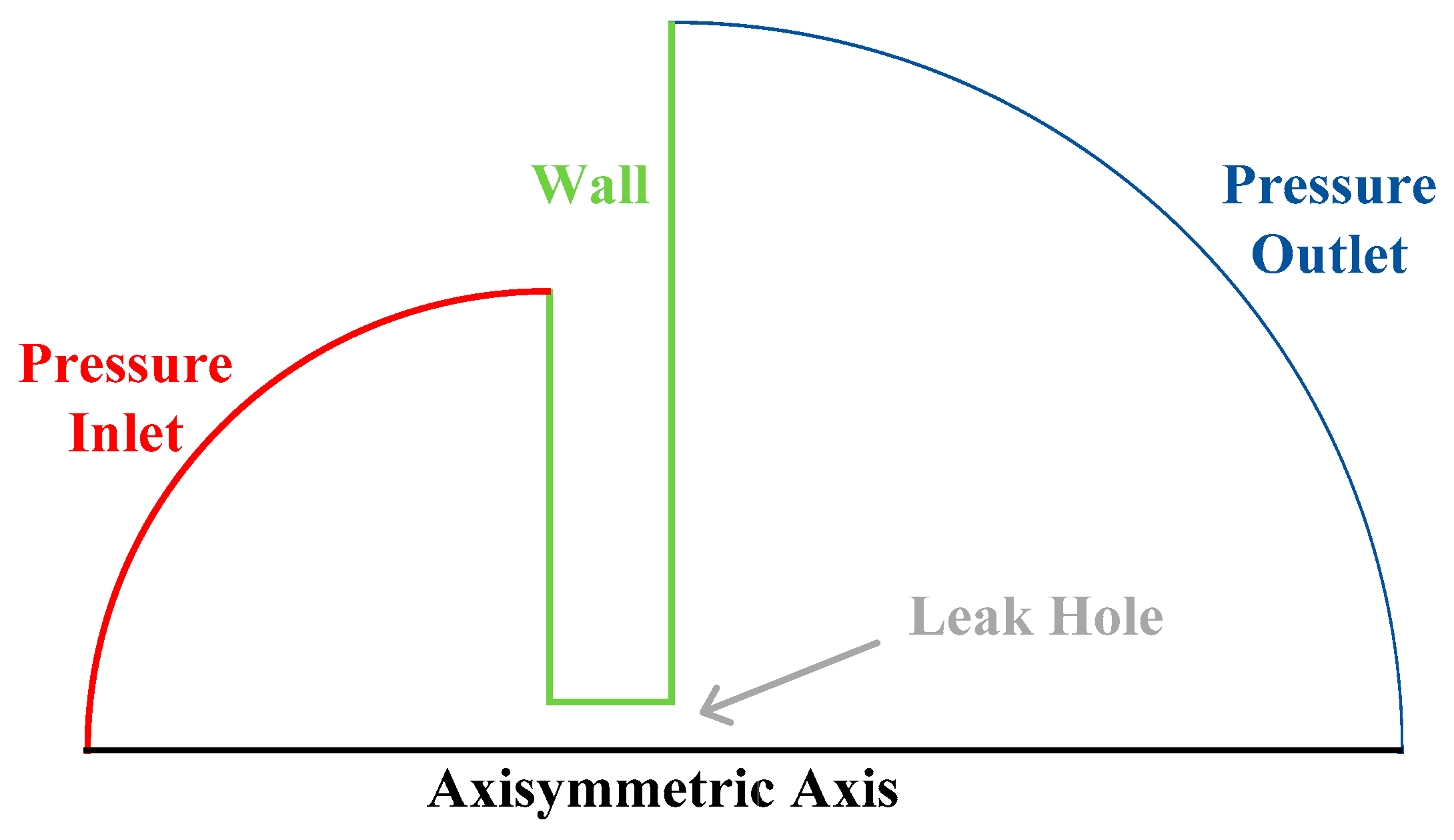
The main pressure vessel of the space station cabin is a cylindrical shell structure with a thickness of 2.5 mm. As leak holes formed by the impact of tiny space debris are generally at the millimeter level, the computation model is simplified to an axisymmetric model with a leak hole of 2.5 mm in length and 2 mm, 1 mm, 0.5 mm in diameter, respectively. The pressure inlet, defined as the 1 atm atmospheric environment is in front of the leak hole, while the pressure outlet, defined as vacuum environment, is after the leak hole. The specific numerical region is depicted in Figure 1 and the commercial CFD software Fluent 19 Ansys Inc., which is located at Southpointe 2600 Ansys Drive Canonsburg, PA 15317, USA, is used in this paper for calculation.
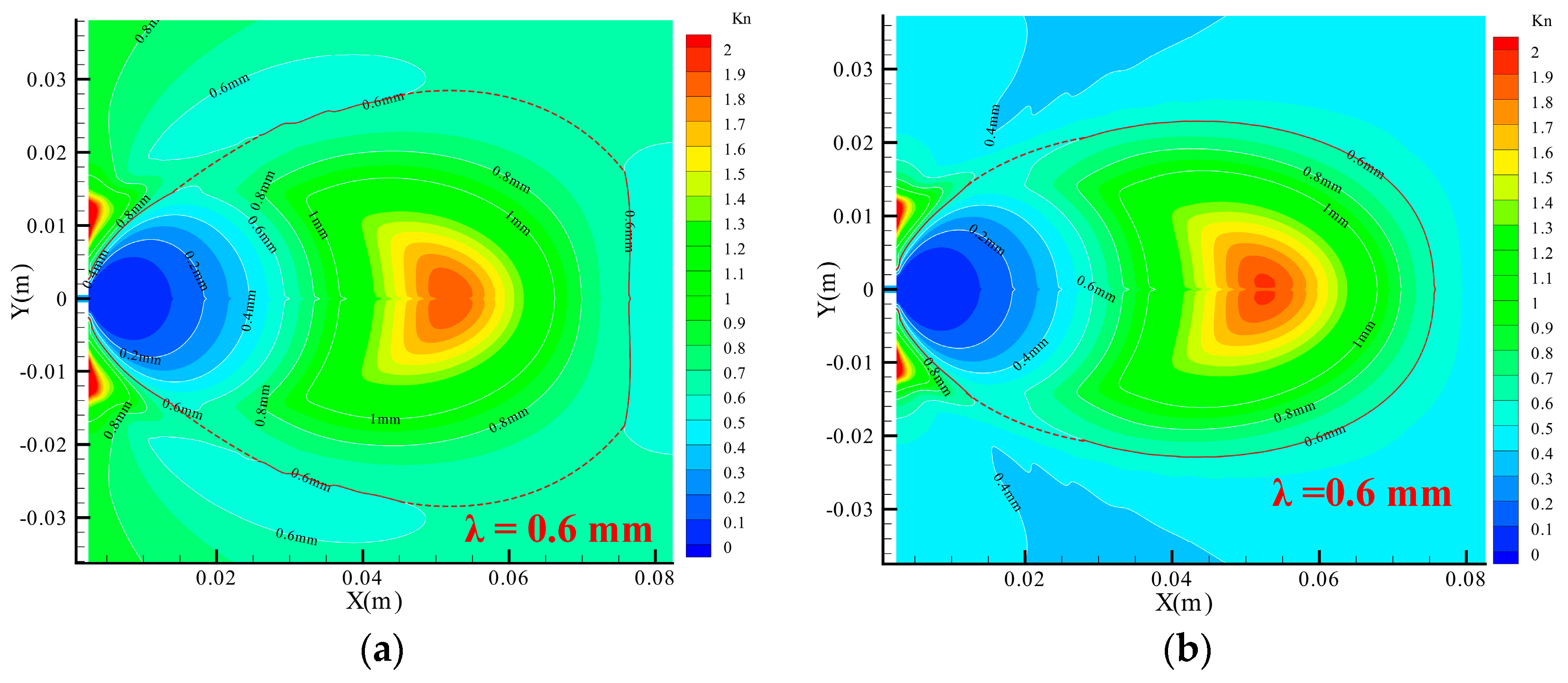
As the ambient pressure on the orbit of the space station is in the order of 10−7~10−4 Pa, the pressure outlet should be set very low to mimic the actual working conditions. However, extremely low setting of outlet pressure imposes high requirements on computational convergence. Besides, the Navier–Stokes (N–S) equations are restricted to describe continuous flow, with limited descriptions of rarefied flow. To fully describe the vacuum jet flow, CFD-DSMC (Computational Fluid Dynamic-Direct Simulation of Monte Carlo) method is widely used. Roughly speaking, the CFD calculation is firstly proceeded to calculate the continuous region and capture the boundary surface between continuous and rarefied region through Knudsen number, denoted by K n . Then, the captured boundary surface is used to initiate the plume field calculation based on DSMC method.
In the numerical calculation, this paper concentrates on the CFD calculation as the acoustic pressure perturbation is mostly related to the continuous fields. To get the convergence, two different configurations of output pressure with 1 Pa and 10 Pa are conducted, where the convergence of steady velocity, pressure, density and temperature is depicted in Figure 2. The results show the difference of aerodynamic properties in continuous region between the two configurations are so minor that they are almost negligible. In other words, under the condition that the back pressure is sufficiently small, the specific value of the back pressure has little effect on the computation accuracy in continuous region. As such, the pressure outlet is set to 10 Pa to improve the computational convergence while the pressure inlet is set to 1 atm to simulate actual pressure condition in the space station cabin.
The temperature in the area in front of the leak hole is uniformly set to 300 K to simulate real thermal condition inside the spacecraft cabin. However, the temperature in orbit is greatly affected by solar radiation so that the temperature range outside the cabin is exceptionally large. In low earth orbit where most spacecrafts work, the temperature in the sun light area can reach above 120 degrees Celsius, while the temperature in the shadow area will quickly drop to below minus 100 degrees Celsius [23]. Therefore, the effect of temperature cannot be neglected. As such, the temperature in the area behind the leak hole is set to 173 K, 300 K and 393 K respectively. In order to explain the dynamic properties and aeroacoustic characteristics, jet in atmospheric environment under the same computational model and pressure difference is also provided, where the pressure inlet and outlet is set to 2 atm and 1 atm respectively, meanwhile other setups remain unchanged.
It is obvious in Figure 2 that the vacuum leak jet is a supersonic flow with a strong density gradient, thus the gas compressibility cannot be neglected. As such, the ideal gas state equation is used in this paper to model the density characteristic of compressible gas, satisfying:
ρ = M p T
where ρ is the density, p is the absolute pressure, T is the static temperature, M is the average molecular weight of air, and is the universal gas constant (taken as 8.31 J mol 1 K 1 ).
As the temperature changes are obvious in the vacuum leak, the fluid viscosity change should be considered. In numerical calculation, the Sutherland equation is introduced to model the viscosity:
μ = μ 0 ( T T 0 ) 3 2 T 0 + S T + S
where μ is the viscosity coefficient, μ 0 is the reference viscosity (taken as 1.716 × 10⁻⁵ kg m 1 s 1 ), T is the static temperature, T 0 is the reference temperature (taken as 273.11 K), and S is the Sutherland constant (taken as 110.56 K).
In terms of numerical calculation, the turbulent characteristics of the jet must be taken into consideration to fully simulate the acoustic characteristics. There are usually three method to calculate a turbulence: Direct Numerical Simulation (DNS), Large Eddy Simulation (LES), and Reynolds Averaged Navier–Stokes (RANS). DNS can obtain the vortex structure on almost every scale by directly solving the N-S equations. But it requires grid number reach Re9/4, which greatly increases the amount of computation. LES uses the N-S equations to directly solve large-scale eddies and imposes the effect of fine-scale vortices on instantaneous motion through various theoretical models. RANS has a weaker resolution of fluctuation terms than DNS and LES, but it has been widely used in the engineering community because of its reliable calculation accuracy, low computation resource requirement, and widely applicable Reynolds number. Therefore, after comprehensive consideration of computation resource and computation precision, a RANS method is used in this paper. Many scholars have proposed a large number of turbulence models to enclose the equations, among which k-ε model has been widely used. Khavaran [24] applied a k-ε model to the computation of supersonic jet mixing noise and successfully predicted the noise source strength. Li X. D. [25] used a modified two-equation standard k-ε model to study a circular jet and not only the predicted shock cell structure and radial density profiles, but also the amplitudes of the flapping and helical modes coincide with the experiments very well. Compared with the standard k-ε model [26], the Realizable k-ε model [27] has higher computation accuracy on jet simulation. As such, the Realizable k-ε model is adopted in this paper with the transport equation being:
t ( ρ k ) + x j ( ρ k u j ) = x j [ ( μ + μ t σ k ) k x j ] + G k + G b ρ ε Y M + S K ,
t ( ρ ε ) + x j ( ρ ε u j ) = x j [ ( μ + μ t σ ε ) ε x j ] + ρ C 1 S ε ρ C 2 ε 2 k + υ ε + C 1 ε ε k C 3 ε G b + S ε
It is shown by Thies [28] that the realizable k-ε model has higher prediction accuracy in solving supersonic turbulent jets where the Mach number is not very large if C 2 ε = 2.02 , σ k = 0.324 , σ ε = 0.377 , Pr = 0.422 , S = 2 S i j S i j , η = S k / ε and C 1 = max [ 0.43 , η / η + 5 ] .
In terms of non-reflecting boundary conditions in aeroacoustic numerical simulation, the common method is to apply appropriate mathematical processing on the boundary conditions to eliminate the reflection on the boundary [29,
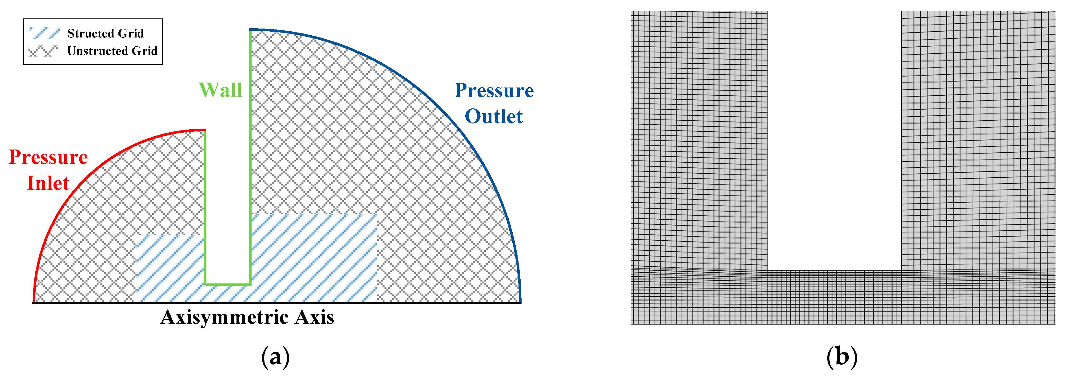
30]. However, it requires a lot of theoretical derivation and programming. A mixed structed–unstructed grid is created in this paper, as shown in Figure 3, where the grid size in the structed area should be small enough to adequately resolve the jet structure and pressure fluctuation meanwhile the grid size in the unstructed area should grow uniformly along the radial direction and be large enough near the inlet and outlet areas. The reason of the grid setup in this paper is to use the numerical viscosity brought about by the change of grid size to dissipate the pressure fluctuation completely before reaching the boundary to avoid the effect of boundary reflection.

3. Discussion

3.1. Comparison of Vacuum and Atmospheric Environment

Whether the external environment is vacuum or atmospheric determines the formation of flow field and the mechanism of perturbation propagation. In this section, a 2 mm leak hole model under different environment is calculated, meanwhile the initial temperature is uniformly set to 300 K in the entire computational domain.

3.1.1. Dynamic Properties

Figure 4 shows the velocity contour of steady leak jet under vacuum environment and atmospheric environment respectively, where the leak hole diameter is 2 mm. For vacuum environment, the gas will expand rapidly through the leak hole into vacuum environment outside and form a supersonic region with Mach 2 to 3. Furthermore, the diameter of the jet potential core is about 25 times the diameter of the leak hole. For atmospheric environment, the jet is a subsonic jet and no obvious expansion is observed. The jet’s diameter is roughly consistent with the diameter of the leak hole.
In a normal atmospheric environment, a supersonic jet will form a series of expansion fans at the exit of the nozzle, which will be reflected when reaching the jet boundary. Then a series of compression waves is formed and constitutes a Mach disk. When the compression waves travel downstream to the jet boundary, the occurrence of reflection induces new expansion fans. Repeated circulation forms a quasi-periodic shock cell structure, as shown in Figure 5. On a micro level, the generation, propagation and reflection of wave systems are essentially due to the collisions of a large number of molecules. When a certain point in the flow field is disturbed, the energy state of surrounding molecules and the probability of collision between molecules will be changed. Energy transfer will occur between molecules once the collision happens. As the disturbance propagates to the surrounding environment, series of directional wave systems are formed.
However, in vacuum environment, the extremely low molecular number density makes the jet quickly transform from a continuous flow to a rarefied flow once the gas enters the vacuum environment. When the expansion fan reaches the jet boundary, it cannot reflect or generate compression wave system because the local molecular number density is far lower than that in the normal atmospheric environment. Therefore, there is no shock cell structure generated in the vacuum environment.
Figure 6 shows the density and pressure distribution of steady leak jet under vacuum environment and atmospheric environment, respectively. It can be seen that the density in vacuum environment shows a shape of droplets, which is in high agreement with the approximate analytical solution of Draper and Hill [10]. Besides, there is a large density gradient in a small area near the leak hole exit, which satisfies the tendency that the closer to the exit center, the larger the density gradient. The density drops rapidly from 0.59 kg/m3 to 0.33 kg/m3 at a distance of 1 mm downstream from the leak hole exit center. As a contract, the change of the density in conventional atmospheric environment is relatively gentle and no strong gradient is observed. The density only decreases from 1.45 kg/m3 to 1.44 kg/m3 at a distance of 1 mm downstream from the leak hole exit center. The pressure in vacuum environment is similar to the density contour, showing a regular droplet shape. A large pressure gradient is also observed in a small area near the leak hole exit with a rapid drop of about 38,000Pa as the expansion fan travels 5 mm downstream. Nevertheless, the pressure change in conventional environment is relatively smooth.

3.1.2. Aeroacoustic Characteristics

Different external space conditions determine completely different acoustic characteristics. As shown in Figure 7, it is obvious that two wave series travel in opposite directions in vacuum environment and cannot reach far field. Why such disturbance propagation is formed in vacuum environment will be discussed in the next section. Nevertheless, in a subsonic jet under atmospheric environment, the compressibility of the gas is weak, which leads to the absences of shock cell structure as well as changes in the characteristic impedance inside and outside the shear layer. So, a directional quadrupole source is formed at the leak hole exit, which continuously radiates to the far field.

3.2. Effect of Leak Hole Size

Leak hole size also has great influence on the dynamic properties and aeroacoustic characteristics. In this section, to explain how leak hole size effect the flow field and why such disturbance is formed, a 1 mm leak hole model and a 0.5 mm leak hole model under the same vacuum environment are calculated, meanwhile the initial temperature is uniformly set to 300 K in the entire computational domain.

3.2.1. Dynamic Properties

Figure 8 shows the velocity contour of steady jet formed by the leak hole of 1 mm and 0.5 mm in diameter, respectively. The diameter of the jet potential core is also about 25 times the leak hole diameter.
Figure 9 shows the density and pressure distribution. In addition to the similar droplet-like shape and large gradient, as the leak hole diameter decreases, the density decreases proportionally to the leak hole diameter in radial direction but shows a flattening trend in the axial direction. The pressure distribution is also similar to the 2 mm leak hole model simulated above and the proportional relation in radial direction and flattening trend in axil direction discovered in the density contour are also observed in the pressure contour map.

3.2.2. Aeroacoustic Characteristics

The essence of sound waves is the transmission phenomenon of pressure disturbances in the medium. Whether a sound wave can propagate from the disturbance source to the far field depends on the existence of a medium. As such, mechanisms of the generation and propagation of supersonic jet noise in atmospheric environment are quite different from those in vacuum environment. In atmospheric environment, the instability waves travel downstream extracting energy from the potential core and making the amplitude grow rapidly. When it interacts with the shock cell structure, strong reflected waves will be generated and travel upstream. The consistent characteristic impedance makes it possible for most energy of the reflected waves to penetrate the shear layer and reach the leak hole lip which is susceptible to external disturbance due to the very thin shear layer. Therefore, new instability wave is excited, travelling downstream and a complete feedback loop is formed, leading to the excitation of screech tones [20].
However, in vacuum environment, the extremely low molecular number density makes the characteristic impedance inside and outside the shear layer very different. So, the instability waves cannot penetrate the shear layer to reach far field, but be reflected upstream along the shear layer and new instability wave is excited at the leak hole lip, thereby forming the feedback loop. The reflection path of pressure fluctuation forms an approximate cavity resonance structure, which is different from the conventional cavity resonance. On the other hand, obvious density, pressure, and temperature gradients existing in vacuum leak jet make the mechanism of sound generation very complicated. Furthermore, the acoustic impedance change also complicates the pressure fluctuation reflection path.
Figure 10 shows the pressure fluctuation contour of different leak hole diameter. It can be seen obviously that for a vacuum leak jet shown in Figure 7a and Figure 10, as the leak hole diameter decreases, both forward waves and backward waves get weaker and weaker. However, there is a certain boundary where a clear reflection phenomenon occurs and the reflected wave feeds back along this boundary.
Knudsen number, K n , which is a dimensionless parameter representing the flow rarefaction, can be used to analyze the vacuum jet. Knudsen number is defined by K n = λ / L , where λ is mean free path of air molecules and L is the characteristic length. Theoretically, λ is calculated by:
λ = k 0 T 2 π d 2 p
where k 0 is Boltzmann constant ( k 0 = 1.38 × 10 23 ) and d is the average diameter of air molecules ( d = 3.74 × 10 10   m ). According to the value of K n , the flow can be divided into four types, namely, K n ≤ 0.01 for continuous flow, 0.01 < K n ≤ 0.1 for slip flow, 0.1 < K n ≤ 10 for transition flow and K n > 10 for molecular flow. Continuous flow and slip flow still satisfy the continuity hypothesis and can still be calculated using the Navier-Stokes (N-S) equation, while the rarefied effect must be considered when computing transition flow and molecular flow. Choosing leak hole diameter as the characteristic length, K n contour is shown in Figure 11.
It can be seen obviously that there is a good agreement between the reflection boundary and K n , where K n = 0.3 for 2 mm leak hole, K n = 0.6 for 1 mm leak hole and K n = 1.2 for 0.5 mm leak hole. Although K n may seem slightly larger than the criterion to distinguish the continuous flow and rarefied flow, where K n = 0.1 , the computational results in this paper is still believed to be reliable. Because characteristic length has a significant influence on K n . For example, the diameter of the nozzle throat is often chosen as the characteristic length when computing the plume field generated by a Laval nozzle using the CFD-DSMC method. The leak hole in this paper is cylindrical, so the range of K n can be appropriately relaxed. Due to the existence of a supersonic region, a silent zone is formed, and the reflected waves cannot propagate across the whole flow field, but propagate upstream clingy to the shear layer. Besides, it is not difficult to find that there is a proportional relationship between the K n criterion and the leak hole diameter. So when only λ is considered, the criterion can be normalized to λ = 0.6   mm , as shown in Figure 11. Hence, the λ criterion seems to be more suitable than the K n criterion to judge the boundary of the acoustic cavity. Although λ = 0.6   mm may not define the cavity wall integrally because of the discontinuity of λ = 0.6   mm , it is apparent that the reflection is intense as long as λ = 0.6   mm exists. The reflected waves within the λ criterion cause resonance phenomenon, partly forming a typical acoustic cavity resonance problem.
Because of the vacuum environment, the sound wave energy cannot be transmitted to the far field. Part of the energy is transmitted to the plume, which is dissipated as the density decreases. Part of the energy is reflected upstream along the acoustic cavity wall (shear layer) and stimulates new instability waves near the leak hole lip area, and then generates multiple resonance modes. Abedi’s group [21,22] conducted a leak-induced jet noise experiment on the ISS and found an obvious resonance phenomenon and harmonic characteristics in the spectrums, which still cannot be explained by any terrestrial jet noise theories. The appearance of the resonance phenomenon confirms that there is indeed a cavity-like structure in the vacuum jet. Furthermore, the limitation of the cavity makes more disturbance waves at different frequencies reflected upstream along the mixing layer. It is bound to excite multiple discrete tones at different frequencies, presenting harmonic characteristics in the spectrums. However, current work can only explain qualitatively why such spectrums under real leak conditions are formed. Further work is still needed to predict precisely when the resonance frequency occurs and how strong the resonance can be.

3.3. Effect of External Thermal Condition

Spacecrafts endure drastic thermal cycles in orbit, resulting in a large temperature range in the outer space. To study whether the λ criterion is still applicable to the real thermal condition in orbit, another two temperature, which is 173 K and 393 K, using 1 mm leak hole model is calculated. Together with 300 K using 1 mm leak model calculated in last section, three examples are analyzed in this section, basically covering the whole temperature range.

3.3.1. Dynamic Properties

The information of downstream cannot travel backwardly to the upstream for a supersonic jet, so the main potential core remains fairly consistent no matter what the outer temperature is, as shown in Figure 8a and Figure 12. However, the subsonic region peripheral to the potential core can still extracting energy from outer thermal condition. As the temperature decreases, the whole flow area also shrinks. High consistence is also observed in density and pressure distribution of different external temperature, as shown in Figure 9a and Figure 13.

3.3.2. Aeroacoustic Characteristics

Figure 14 shows the pressure fluctuation contour of different external temperature. It is obvious that the external temperature does not change the fluctuation propagation as significantly as the leak hole diameter. The opposing fluctuation waves still propagate at approximately the same position with approximately the same intensity.
By analyzing the K n distribution and λ distribution shown in Figure 15, it can be seen that although changes in external temperature brings about noteworthy changes in K n distribution, the boundary defined by λ = 0.6   mm remains high similarity, that is, the acoustic cavity is not affected by external temperature, and then accounting for the applicability of λ criterion in real on-orbit condition.

4. Conclusions

The realizable k-ε model is adopted in this paper to numerically simulate the aerodynamic properties and aeroacoustic characteristics of a leak-induced jet with different external environment, different leak hole diameter and different external thermal condition. Numerical results show that:
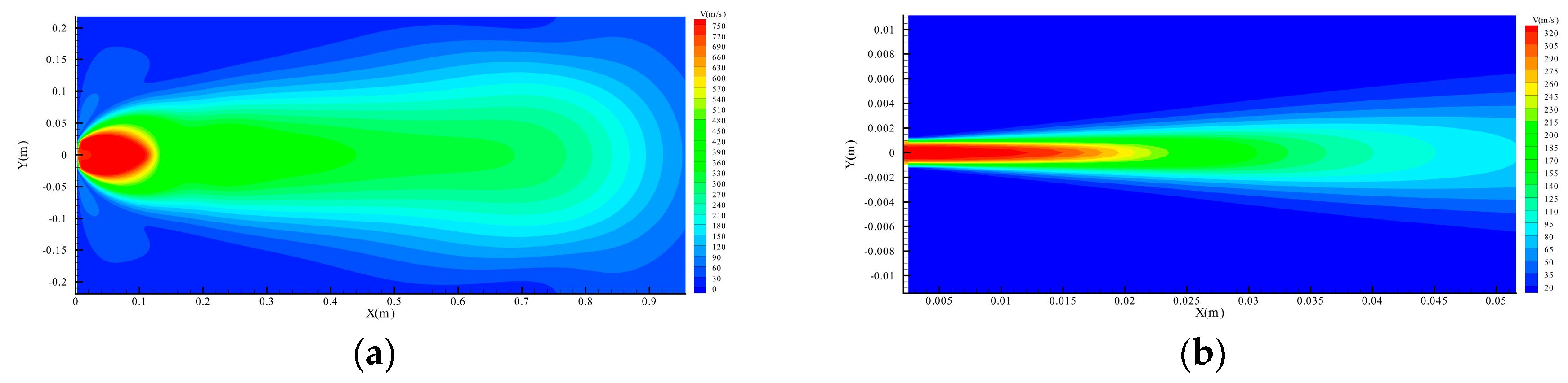
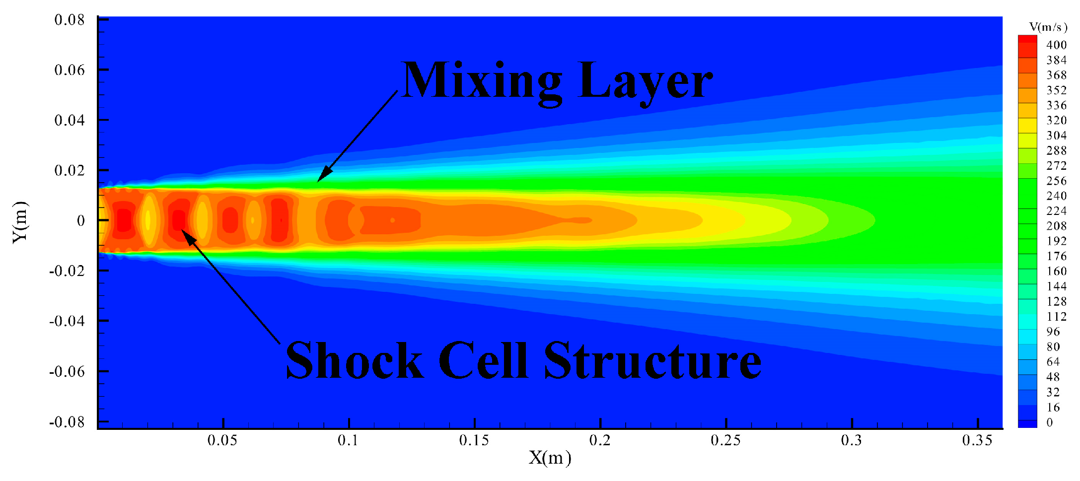
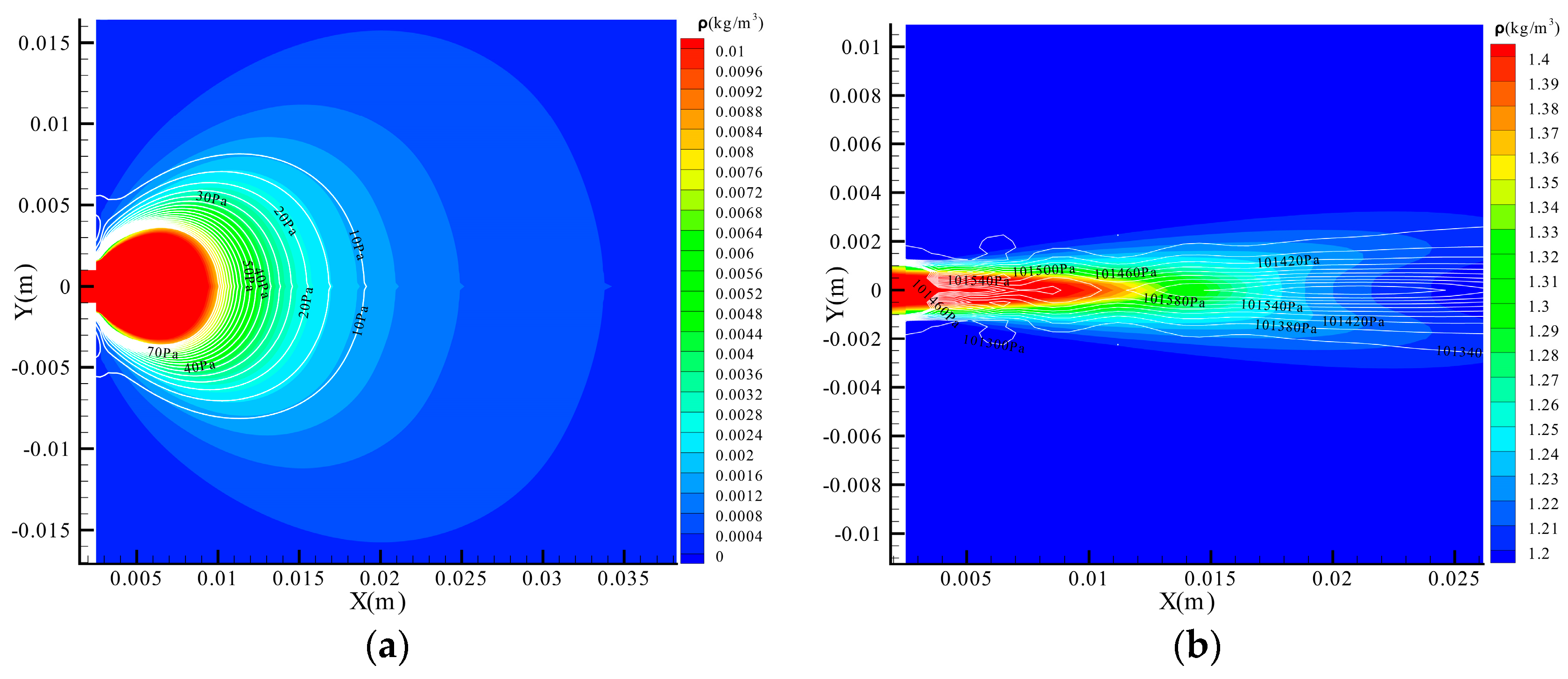
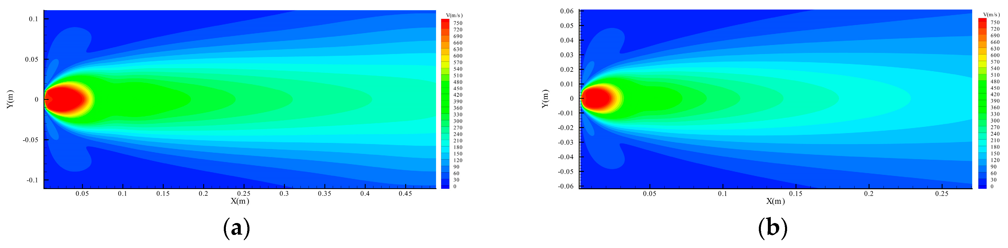
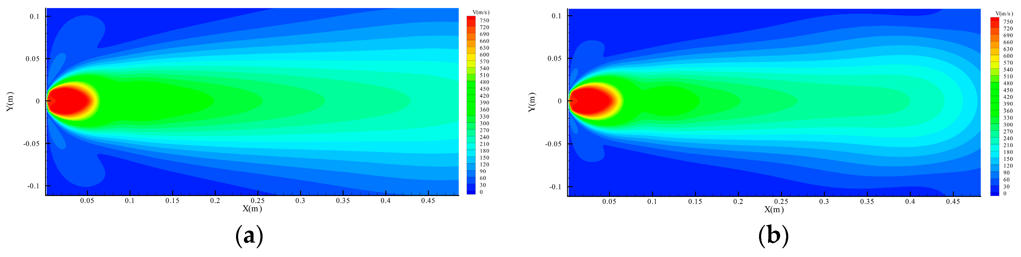
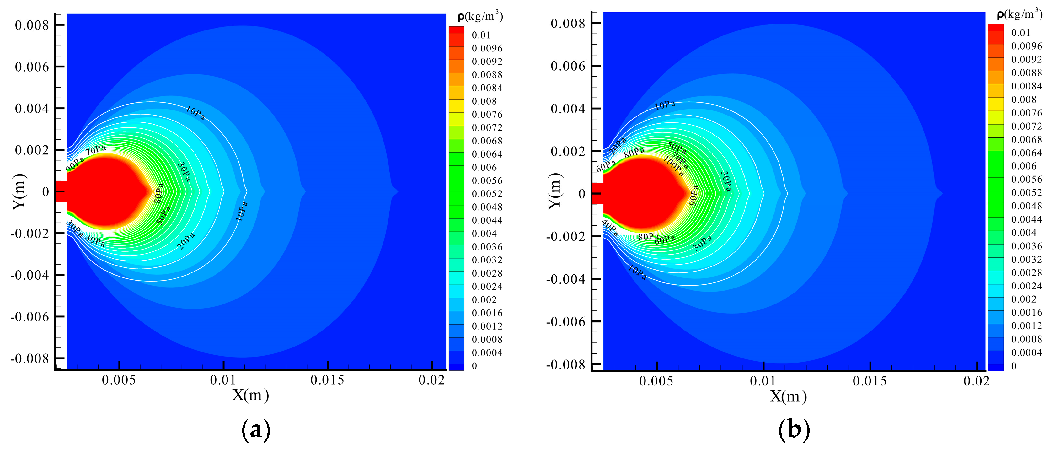
(1) On the space station, the leak gas will expand into outer vacuum space rapidly and form a supersonic jet with a Mach number of 2 to 3, the diameter of the jet potential core being about 25 times the diameter of the leak hole. Although there are large velocity, density, pressure, and temperature gradients, no typical shock cell structure is observed. In contract, conventional terrestrial leak jet under the same pressure difference of 1 atm is still subsonic and no obvious expansion can be seen.
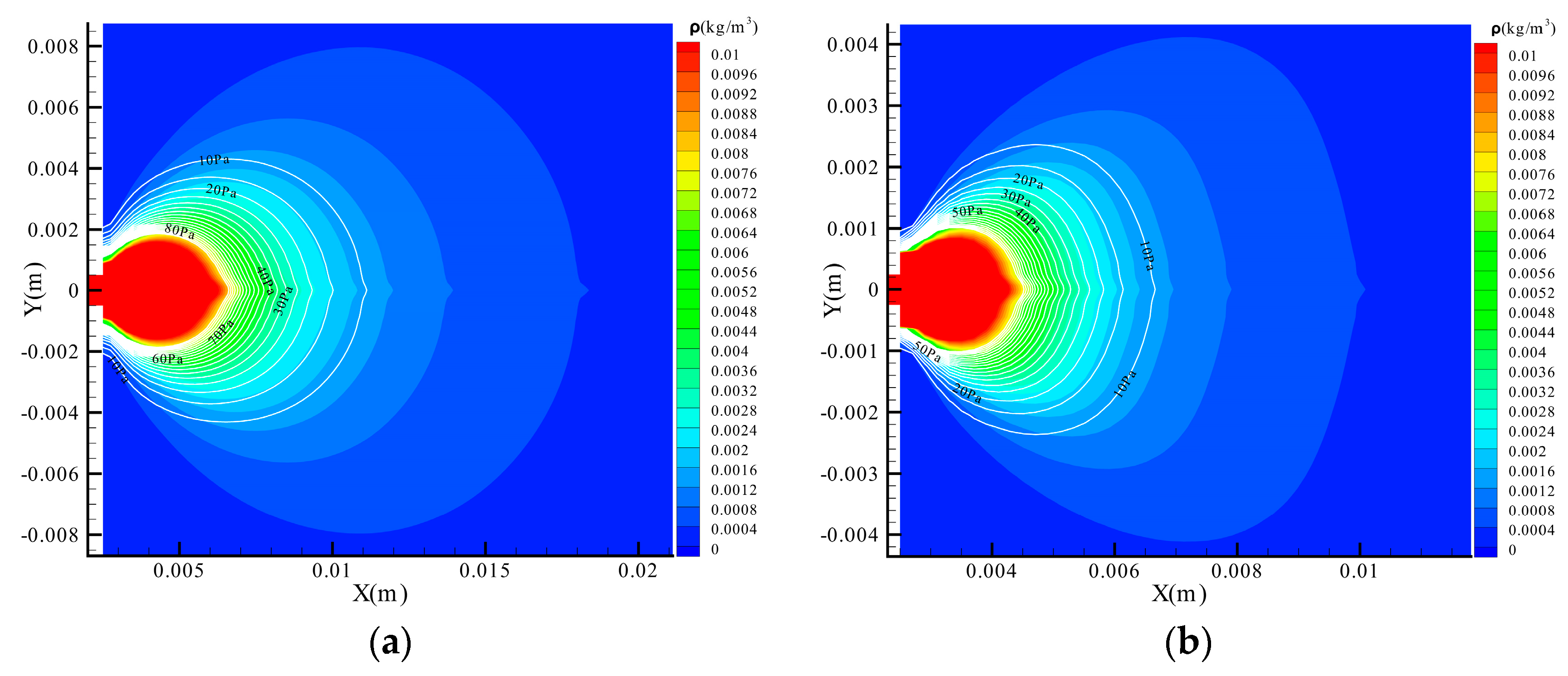
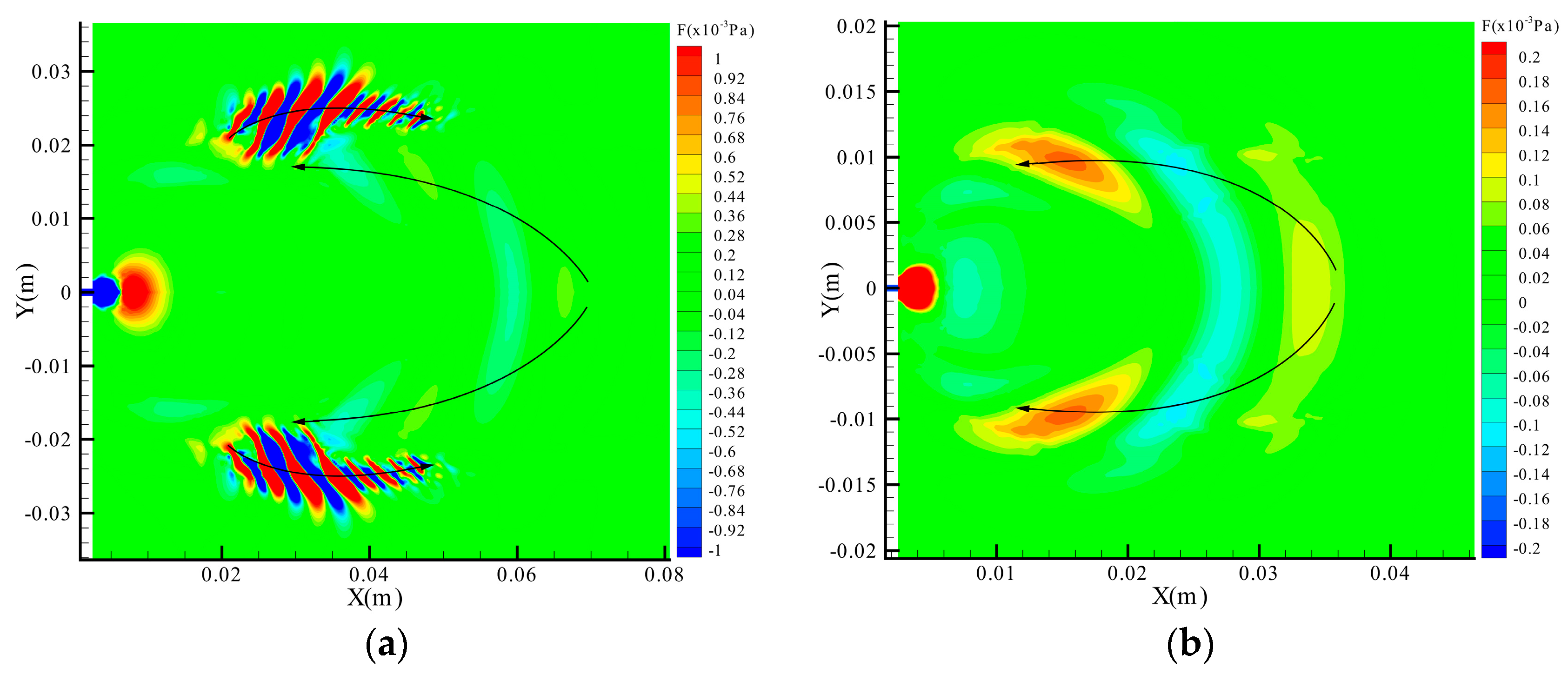
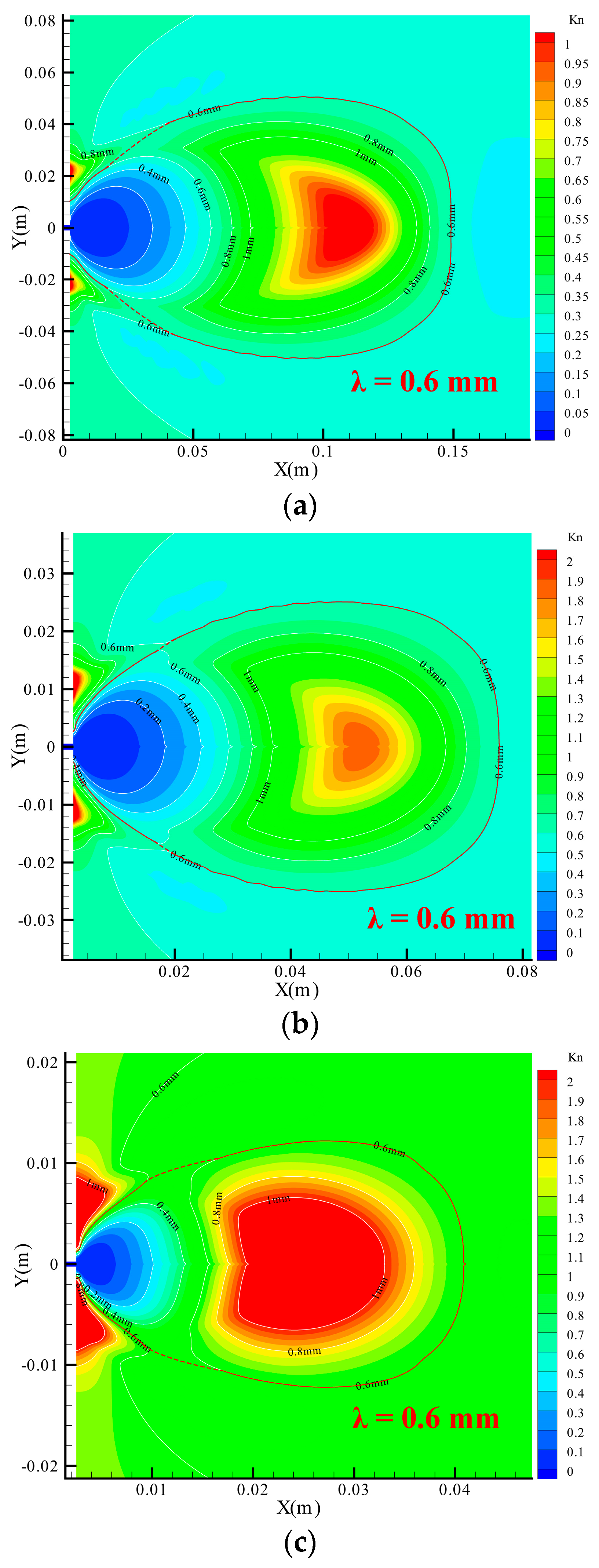
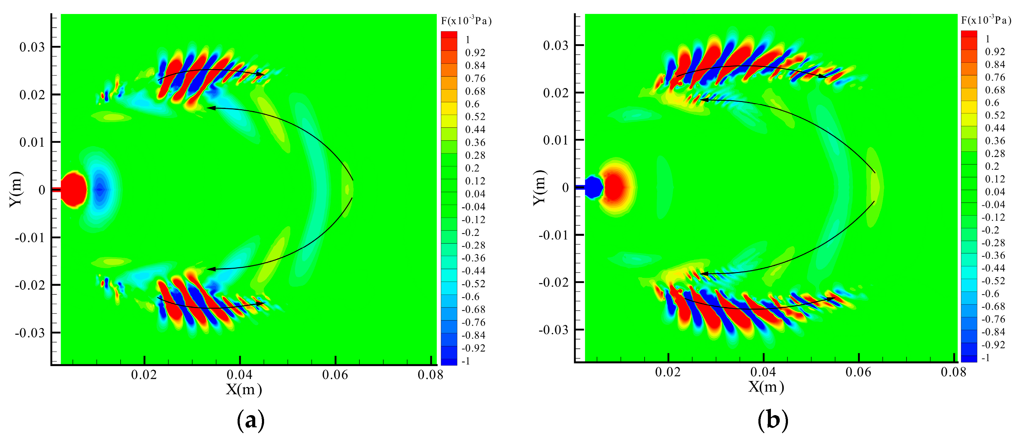
(2) The jet noise in vacuum environment shows a phenomenon of acoustic cavity reflection. Compared with widely used K n criterion in vacuum plume dynamics, the λ criterion seems more appropriate to define the acoustic cavity wall. Within the acoustic cavity which is judged by λ = 0.6   mm , the reflected waves reflect upstream along the acoustic cavity wall, exciting multiple resonance harmonic modes. Interestingly, the λ criterion is universally suitable for different leak hole diameter and external temperature, which may confront in the on-orbit applications. In addition, it is not difficult to find that the source of vacuum leak jet noise is mainly composed of turbulent mixing broadband noise and resonance harmonic noise.
(3) Although the RANS method’s weaker resolution of the fluctuation terms makes it unable to accurately describe the turbulent mixing broadband noise, it still has a high resolution of the jet dynamic properties and the time-averaged characteristics of pressure disturbance propagation. Furthermore, the computation resource requirement is relatively small. Therefore, RANS method can effectively analyze the characteristics of harmonic noise caused by resonance.

Author Contributions

Y.C. participated in the design of this study. R.-F.Z. conducted the numerical simulation under the guidance of Y.C. L.Q. provided important background information of this problem. X.Z. gave important suggestions on the improvement of simulation. Z.-Y.W. helped the numerical simulation. Y.C. and R.-F.Z. conducted the manuscript preparation. The other authors reviewed the manuscript carefully. All authors read and approved the content of the manuscript.

Funding

This research was funded by the Training Program of the Major Research Plan of the National Natural Science Foundation of China grant number 91741107.

Conflicts of Interest

The authors declare no conflict of interest.

References

  1. Liou, J.C. Risks from orbital debris and space situational awareness. In Proceedings of the 2nd AIAA Conference on Space Situational Awareness, Washington, DC, USA, 14–16 January 2020. [Google Scholar]
  2. Hui, T.L.; Liu, G.; Jia, D.Y.; Yang, C.; Sun, G.H. Assumption on leak monitoring and alarming for space station absolute pressure leak detection. Manned Spacefl. 2012, 18, 36–41. [Google Scholar]
  3. Liu, W.P.; Wang, M.Q. Gas Leak Detection by Differential Pressure Method. Mech. Eng. Autom. 2010, 158, 133–135. [Google Scholar] [CrossRef]
  4. Dirk, A.; Alex, C.; Steve, W.; Karen, H. Acoustic emission source location on large plate-like structures using a local triangular sensor array. Mech. Syst. Signal Pr. 2012, 30, 91–102. [Google Scholar]
  5. Friesel, M.A.; Barga, R.S.; Dawson, J.F.; Hutton, P.H.; Kurtz, R.J.; Lemon, D.K. Acoustic emissions applications on the NASA Space Station. NDT E Int. 1991, 27, 725–732. [Google Scholar]
  6. William, C.W.; Neil, C.C.; Eric, I.M. Leak detection and location technology assessment for aerospace applications. In NASA/TM-2008-215347; 2008. Available online: https://ntrs.nasa.gov/search.jsp?R=20080041598 (accessed on 22 May 2020).
  7. Holland, S.D.; Roberts, R.; Chimenti, D.E.; Song, J.H. An ultrasonic array sensor for spacecraft leak direction finding. Ultrasonics 2006, 45, 121–126. [Google Scholar] [CrossRef] [Green Version]
  8. Schafer, F.; Janovsky, R. Impact sensor network for detection of hypervelocity impacts on spacecraft. Acta Astronaut. 2007, 61, 901–911. [Google Scholar] [CrossRef]
  9. Reusser, R.S.; Holland, S.D.; Chimenti, D.E.; Roberts, R. Reflection and transmission of guided ultrasonic plate waves by vertical stiffeners. J. Acoust. Soc. Am. 2014, 136, 170–182. [Google Scholar] [CrossRef]
  10. Draper, J.S.; Hill, J.A.F. Analytical approximation for the flow from a nozzle into a vacuum. J. Spacecraft Rockets. 1966, 3, 1552–1554. [Google Scholar] [CrossRef]
  11. Shuvalov, V.A.; Levkovich, O.A.; Kochubei, G.S. Approximate Models of Exhaustion of a Supersonic Gas Jet into Vacuum. J. Appl. Mech. Tech. Phys. 2001, 42, 237–242. [Google Scholar] [CrossRef]
  12. Kannenberg, K.C.; Boyd, I.D. Three-dimensional Monte Carlo simulations of plume impingement. J. Thermophy. Heat Tr. 1999, 13, 226–235. [Google Scholar] [CrossRef]
  13. Lighthill, M.J. Jet noise. AIAA J. 1963, 1, 1507–1517. [Google Scholar] [CrossRef]
  14. Ffowcs, W.J.E. The acoustic analogy—Thirty years on. IMA J. Appl. Math. 1984, 32, 113–124. [Google Scholar]
  15. Farassat, F. Acoustic radiation from rotating blades—The Kirchhoff method in aeroacoustics. J. Sound Vib. 2001, 239, 785–800. [Google Scholar] [CrossRef] [Green Version]
  16. Phillips, O.M. On the generation of sound by supersonic turbulent shear layers. J. Fluid Mech. Digit. Arch. 1960, 9, 1–28. [Google Scholar] [CrossRef]
  17. Goldstein, M.E. A generalized acoustic analogy. J. Fluid Mech. 2003, 488, 315–333. [Google Scholar] [CrossRef] [Green Version]
  18. Tam, C.K.W.; Golebiowski. On the two components of turbulent mixing noise from supersonic jets. In Proceedings of the 2nd AIAA/CEAS Aeroacoustics Conference, Pennsylvania, PA, USA, 6–8 May 1996. [Google Scholar]
  19. Tam, C.K.W.; Chen, P. Turbulent mixing noise from supersonic jets. AIAA J. 1994, 32, 1774–1780. [Google Scholar] [CrossRef]
  20. Tam, C.K.W. Supersonic jet noise. Annu. Rev. Fluid Mech. 1995, 27, 17–43. [Google Scholar] [CrossRef]
  21. Clark, C.; Labonte, L.; Castro, J.; Abeli, A.; Caccese, V. Wireless leak detection using airborne ultrasonics and a fast-bayesian tree search algorithm with technology demonstration on the ISS. In Proceedings of the 2015 IEEE International Conference on Wireless for Space and Extreme Environments (WiSEE), Orlando, FL, USA, 14–16 December 2015. [Google Scholar]
  22. Bundy, K.R.; Pandian, C.M.; Abedi, A.; Caccese, V. Analysis of leak spectral signatures in pressurized space modules. In Proceedings of the 2016 IEEE International Conference on Wireless for Space and Extreme Environments, Aachen, Germany, 26–28 September 2016. [Google Scholar]
  23. Wu, L. The dynamic Study and Thermal Protection Technology of Driving Devices for Spacesuit Test. Master’s Thesis, Beijing Jiaotong University, Beijing, China, 2012. [Google Scholar]
  24. Khavaran, A.; Krejsa, E.A.; Kim, C.M. Computation of supersonic jet mixing noise for an axisymmetric CD nozzle using k-epsilon turbulence model. In Proceedings of the 30th Aerospace Sciences Meeting & Exhibit, Reno, NV, USA, 6–9 January 1992. [Google Scholar]
  25. Li, X.D.; Gao, J.H. Numerical simulation of the three-dimensional screech phenomenon from a circular jet. Phys. Fluids. 2008, 20, 35101. [Google Scholar] [CrossRef]
  26. Cheng, Y.; Lien, F.S.; Yee, E.; Sinclair, R. A comparison of large Eddy simulations with a standard k-ε Reynolds-averaged Navier-Stokes model for the prediction of a fully developed turbulent flow over a matrix of cubes. J. Wind Eng. Ind. Aerod. 2003, 91, 1301–1328. [Google Scholar] [CrossRef]
  27. Shih, T.H.; Liou, W.W.; Shabbir, A.; Yang, Z.; Zhu, J. A new k- ε eddy viscosity model for high reynolds number turbulent flows. Comput. Fluids. 1995, 24, 227–238. [Google Scholar] [CrossRef]
  28. Thies, A.T.; Tam, C.K.W. Computation of turbulent axisymmetric and nonaxisymmetric jet flows using the K-epsilon model. AIAA J. 1996, 34, 309–316. [Google Scholar] [CrossRef]
  29. Loh, C.Y.; Hultgren, L.S.; Chang, S.C.; Jorgenson, P.C.E. Noise computation of a shock-containing supersonic axisymmetric jet by the CE/SE method. In Proceedings of the 38th Aerospace Sciences Meeting & Exhibit, Reno, NV, USA, 10–13 January 2000. [Google Scholar]
  30. Loh, C.Y.; Hultgren, L.S.; Chang, S.C.; Jorgenson, P.C.E. Near field noise computation for an underexpanded supersonic jet by the CE/SE method. In Proceedings of the 7th AIAA Aeroacoustics Conference, Maastricht, The Netherlands, 28–30 May 2001. [Google Scholar]
Figure 1. Schematic diagram of the computational model.
Applsci 10 03640 g001
Figure 2. Comparison of axial aerodynamic properties under different back pressure. (a) velocity; (b) pressure; (c) density; (d) temperature.
Applsci 10 03640 g002
Figure 3. Grid model. (a) schematic diagram of the grid model; (b) grid around the leak hole (take the 2 mm leak hole model as example).
Applsci 10 03640 g003
Figure 4. Velocity contour of different external environment. (a) vacuum environment; (b) atmospheric environment.
Applsci 10 03640 g004
Figure 5. Shock cell structure and mixing layer in a supersonic jet.
Applsci 10 03640 g005
Figure 6. Density contour with pressure contour map of different external environment. (a) vacuum environment; (b) atmospheric environment.
Applsci 10 03640 g006
Figure 7. Pressure fluctuation contour of different external environment (The arrow marked in the figure represents the direction of fluctuation wave propagation.). (a) vacuum environment; (b) atmospheric environment.
Applsci 10 03640 g007
Figure 8. Velocity contour of different leak hole diameter. (a) 1 mm; (b) 0.5 mm.
Applsci 10 03640 g008
Figure 9. Density contour with pressure contour map of different leak hole diameter. (a) 1 mm; (b) 0.5 mm.
Applsci 10 03640 g009
Figure 10. Pressure fluctuation contour of different leak hole diameter (The arrow marked in the figure represents the direction of fluctuation wave propagation.). (a) 1 mm; (b) 0.5 mm.
Applsci 10 03640 g010
Figure 11. K n contour with λ contour map of different leak hole diameter (The red line marked in the figure represents λ = 0.6   mm and the dotted line is an imaginary line to fix the discontinuity). (a) 2 mm; (b) 1 mm; (c) 0.5 mm.
Applsci 10 03640 g011
Figure 12. Velocity contour of different external temperature. (a) 393 K; (b) 173 K.
Applsci 10 03640 g012
Figure 13. Density contour with pressure contour map of different external temperature. (a) 393 K; (b) 173 K.
Applsci 10 03640 g013
Figure 14. Pressure fluctuation contour of different external temperature (The arrow marked in the figure represents the direction of fluctuation wave propagation.). (a) 393 K; (b) 173 K.
Applsci 10 03640 g014
Figure 15. K n contour with λ contour map of different external temperature (The red line marked in the figure represents λ = 0.6   mm and the dotted line is an imaginary line to fix the discontinuity). (a) 393 K; (b) 173 K.
Applsci 10 03640 g015

