An Image Processing Method for Extraction of the Stress Wave Reflection Period

Abstract

The stress wave reflection method is widely used in the detection of structure size and integrity due to its advantages of low environmental impact and convenience. The detection accuracy depends on the accurate extraction of the stress wave reflection period. The traditional peak–peak method (PPM) measures the time interval between the first two peaks of the reflected waves to extract the reflection period. However, human interpretation is not avoidable for identifying the weak peak due to signal energy leaks into the surrounding environment. This paper proposes an algorithm for automatic extraction of the stress wave reflection period based on image processing to avoid human interference. The image is the short-time Fourier transform (STFT) spectrogram of the reflected wave signal after applying wavelet denoising and quadratic self-correlation operations. The edge detection method of image processing is used to extract the periodically occurring trough in the image. Graying and filtering are performed to eliminate interference. The frequency of the trough distribution is calculated by using the fast Fourier transform (FFT), and then the reflection period of the stress wave is obtained. The effectiveness and accuracy of the proposed method are validated by measuring the different lengths of two buried metal piles in soil. Comparing with the existing method of extracting the stress wave reflection period, this new algorithm comprehensively utilizes the time–frequency domain information of the stress wave reflection signal.

1. Introduction

Underground structures, such as foundation piles, anchor rods, and buried metal piles, play an important role in large civil engineering. The measurement and evaluation of their structural size and integrity are directly related to the safety of the engineered structures. The traditional method, i.e., pull-out testing, can accurately obtain the buried depth and integrity information of the column. However, it is slow in detection speed, low in efficiency, and it has a problem of secondary buried depth. Therefore, nondestructive testing (NDT) methods have been widely used in detecting size and structural health monitoring (SHM).

As an NDT method, the stress wave reflection method has been successfully applied in the health monitoring of foundation piles [1], rock bolts [2,3,4], buried metal piles [5], and pipes [6]. The stress wave reflection method is based on the elastic vibration theory of wave propagation in one-dimensional rods [7]. After impacting upon the top of the pile, the stress wave will reflect when it meets a defect or the end face of the pile in the process of propagation. By detecting and analyzing the travel time, the amplitude and phase characteristics of the reflected waves, as well as the length and damage location of the pile can be detected.

The stress wave is usually produced by piezoelectric materials [8] or vibration hammers [9,10]. Piezoelectric material, e.g., lead zirconate titanate (PZT), as a type of smart material, has attracted a lot of attention in the field of SHM for its small size, high stability, and good linearity. Because piezoelectric materials have direct and inverse piezoelectric effects, they can be used as both a vibrator and a sensor. PZT-based sensors have been successfully applied to detect metal cracks [11], bolt looseness [12,13], pipelines length [14,15], bond-slip monitoring of concrete structures [16], and so on. Hei et al. [17] proposed using a single piezoelectric ceramic transducer to quantitatively evaluate the bolt connection status. Zhang et al. [18] used three PZT patches as sensors and actuators to form different detection processes to monitor the looseness of the steel strand. In addition, PZT-based stress wave communication in submarine environments may have greater potential than many conventional methods [19]. In this paper, the PZT sensor is used to collect the reflection signals after the hand-held hammer impacts the buried metal pile.

The key to detecting the structural size or defect location by using stress wave reflection is the extraction of the reflection period. The traditional methods of reflection period extraction include the peak–peak method (PPM) and phase analysis method (PAM). The PPM finds the first two peaks of the reflected wave and takes the time interval between the two peaks as the reflection period; however, this method is only applicable to measurement signals with obvious periodic reflection. Tiwari et al. [20] detected the amplitude of the signal after wavelet denoising to estimate the size and location of the disbond-type defect presented on glass fiber reinforced plastic material. However, when the cylinder is long, the stress wave energy leaks into the surrounding soil during the propagation, which makes the reflected signal too small to evaluate. On the other hand, PAM is widely used to detect bolt length due to the phase mutations only occurring at the end face or defect [21]. Luo et al. [22] analyzed the instant phase of the stress wave to successfully detect the length of the anchor bolt and location of the density defect. However, the interpretation of data depends on skilled personnel and thus has limited objectivity. The self-correlation can make period extraction easier; however, the reflection signal is not obvious due to the energy attenuation and noise interference during wave propagation. The signal period is still difficult to evaluate, even after a single self-correlation. Lei et al. [23] carried out a self-correlation operation and applied statistical operation to develop an automatic extraction algorithm for measuring the length of an in-service rock bolt. The peak position occurrence for multiple measurement signal waves after the self-correlation operation was estimated by statistical method. This method reduced the average error to 2.1% with multiple measurements compared to the PAM average error of 3.1%.

Time–frequency analysis based on image processing for feature extraction has been used in equipment fault detection [24], medical diagnosis [25,26], radar signal recognition [27,28], and nondestructive testing [29,30,31], etc. Ma et al. [28] proposed a self-correlation characteristic image construction technique (ACFICT) combined with a convolutional neural network (CNN) to realize the classification of radar signal modulation types. The authors used the self-correlation algorithm in the step of signal preprocessing and time–frequency image feature enhancement, which makes the algorithm adapt to the feature image during a low signal–noise ratio (SNR) signal. Obuchowski et al. [29] utilized the weight vector to enhance the information features of the time–frequency image, and then extracted and analyzed the local maxima in the frequency domain along the time direction for damage detection in rotating machines. The local increase in amplitude may relate to the pulse disturbance caused by damage. Tian et al. [30] extracted invariant moment features from the adaptive time–frequency distribution map. Li et al. [31] generated a time–frequency spectrogram from the detection signals of a vehicle–bridge interaction and analyzed the change in instantaneous frequency to evaluate the state of the bridge. These methods mainly extract the feature points of the time–frequency spectrogram, but do not study the pixel distribution rule of the whole time–frequency spectrogram. However, the period of pixel distribution in the time–frequency spectrogram is found to be related to the reflection signal period in this research.

In this paper, a new algorithm for the automatic extraction of the stress wave reflection period based on image processing of a time–frequency spectrogram is presented. The image is the short-time Fourier transform (STFT) spectrogram of the reflected wave signal after applying wavelet denoising and quadratic self-correlation operations. The reflection period is calculated by using the relationship between the period of pixel distribution in the time–frequency spectrogram. To the best of our knowledge, there is no study retrieving the stress wave reflection period based on image processing. The validity of the algorithm is verified by a length measurement experiment of metal piles buried under varying depths.

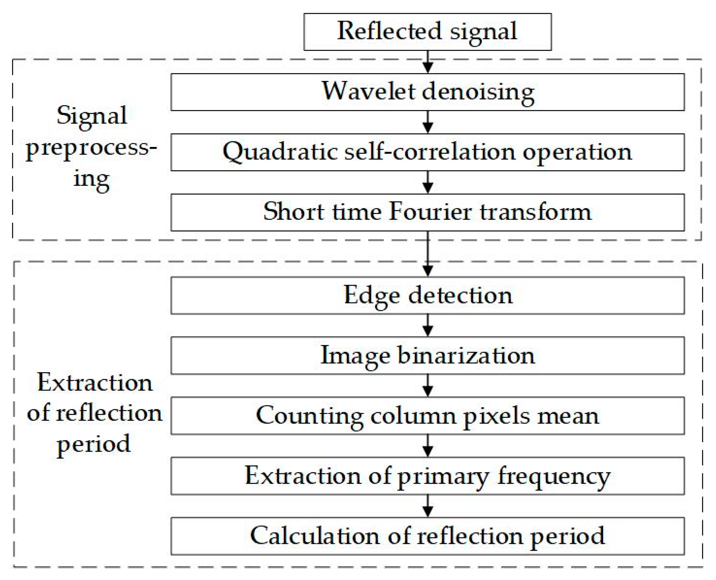
2. Algorithm for the Automatic Extraction of the Reflection Period Based on Image Processing

The algorithm is divided into two parts: signal preprocessing, which generates the time–frequency spectrogram of the stress wave, and extraction of the reflection period. The flow diagram is shown in Figure 1. Signal preprocessing to generate the time–frequency spectrogram includes wavelet denoising, quadratic self-correlation, and STFT. The extraction of the reflection period in the time–frequency spectrogram uses image processing algorithms, i.e., edge detection, grayscale, and binarization. Then, the averages of the column pixels of the binary image is counted to obtain a pixel distribution curve. Self-correlation is performed on the distribution curve to improve the SNR. Finally, the fast Fourier transform (FFT) is used for spectrum analysis to find the frequency corresponding to the maximum amplitude (except for the zero frequency); that is, the primary frequency of the image pixel distribution. The steps are outlined below.

2.1. Step 1: Wavelet Denoising

The multi-resolution wavelet analysis decomposes the signal into different scales and splits the mixed signal into sub-signals of different frequency bands. The decomposition and reconstruction of the wavelet transform are used for signal denoising: decomposing the noise-containing signal into different frequency bands at a certain scale, and then the high-frequency band in which the noise is located is eliminated. The low-frequency coefficients are used for signal reconstruction. The wavelet basis selected for wavelet denoising is Daubechies. In order to give consideration to the calculation amount and the denoising effect, the number of decomposition layers was set to 6. This number was determined by experiments, and the high frequency coefficient of the 6th layer component was removed during the reconstruction.

2.2. Step 2: Quadratic Self-Correlation Operation

The quadratic self-correlation method repeats the self-correlation operation on the result of the self-correlation operation. When there are periodic components in the function, the extremum of the self-correlation function can well reflect this periodicity. The traditional self-correlation detection method is to convolute the input signal and the delayed input signal. Assuming the discrete signal is $\begin{array}{cc}y(k)=s(k)+n(k)& k=1,2,\dots ,K\end{array}$ and that the target signal is $s(k)$, the noise signal is $n(k)$, and $K$ is the number of sampling points. Then the self-correlation function of $y(k)$ is

$$\begin{array}{l}{\mathrm{R}}_{yy}(m)={\displaystyle \sum _{k=0}^{K}y(k)y(k-m)}\\ ={\displaystyle \sum _{k=0}^{+\infty }[s(k)+n(k)][s(k-m)}+n(k-m)]\\ ={\displaystyle \sum _{k=0}^{K}s(k)s(k-m)}+{\displaystyle \sum _{k=0}^{K}s(k)n(k-m)}+{\displaystyle \sum _{k=0}^{K}n(k)s(k-m)}+{\displaystyle \sum _{k=0}^{K}n(k)n(k-m)}\\ =R_{ss}(m)+R_{sn}(m)+R_{ns}(m)+R_{nn}(m)\end{array}$$

(1)

where $R_{ss}(m)$ represents the self-correlation result of the target signal and $R_{nn}(m)$ is the self-correlation function of the noisy signal. $R_{sn}(m)\hspace{0.17em}\mathrm{and}\hspace{0.17em}{R}_{ns}(m)$ represent the correlation result of the target signal and noise, respectively. Due to the non-correlation of the signal and noise as well as noise and noise, the values of $R_{sn}(m),R_{ns}(m),R_{nn}(m)$ are zero. By performing quadratic self-correlation operations on the signal after wavelet denoising, one enhances the periodicity. For signals with a low SNR, its periodicity can be obtained by applying multiple self-correlations.

2.3. Step 3: Generate a Time–Frequency Spectrogram by STFT

STFT is used to determine the frequency and phase of a local-region sine wave of a time-varying signal. For the original signal sequence $\begin{array}{cc}f(k)& k=1,2,\dots ,K\end{array}$, a time–frequency localized window function is selected, and the analysis window function sequence $g(k-m)$ is assumed to be stationary (pseudo-stationary) over a short interval. Moving the window function $g(k-m)$ makes the product of sequence $f(k)$ and sequence $g(k-m)$ be stationary in different window widths, so as to calculate the power spectrum at different times. In simple terms, the process of calculating the STFT is to divide a longer time signal into shorter segments of the same length and to calculate the Fourier transform on each of the shorter segments. The formula is as follows:

$$STF{T}_{f(k)}(e^{j\frac{2n\pi }{N}})={\displaystyle \sum _{m=0}^{K}f(m)g(k-m)e^{-j\frac{2n\pi }{N}m}},0\le n\le N-1,$$

(2)

where $K$ is the number of sampling points, and $N$ is the sampling rate of the discrete signal.

By comparing the time–frequency spectrogram generated by selecting different window functions, the window function of STFT is chosen as Hamming (W/4), where W is the number of sampling bins and is set to 64.

2.4. Step 4: Edge Detection

The Sobel operator is a discrete differentiation operator mainly used for edge detection. It combines Gaussian smoothing and differential derivation to calculate the approximate gradient of the image. Using this operator at any point in the image will produce the corresponding gradient vector or its normal vector. Since the bottom reflection signal appears periodically in time corresponding to the X-axis (time axis) of the time–frequency spectrogram, it is only necessary to detect edge information that changes horizontally on the image. When the Sobel operator kernel size is 3, the kernel matrix in the X direction is

$$Kerne{l}_X=\left[\begin{array}{ccc}-1& 0& 1\\ -2& 0& 2\\ -1& 0& 1\end{array}\right].$$

(3)

Using the kernel matrix to convolve with the original image matrix, the X-direction edge information of the original image is obtained. $I_{src}$ represents the original image matrix, and $I_X$ represents the result of the X-direction edge detection on the original image. The formula is as follows:

$$I_X=Kerne{l}_X\ast I_{src}.$$

(4)

2.5. Step 5: Image Binarization

Since the object of the binarization operation is a grayscale image, it is necessary to grayscale the color image. The method of image graying is a maximum value method, which takes the maximum values of the R, G, and B components in the color image as the values of the gray image, as shown in Equation (5).

$$I_X^{’}(i,j)=\max (R(i,j),G(i,j),B(i,j)),$$

(5)

where $I_X^{’}$ represents the grayscale image of $I_X$, and $R(i,j),G(i,j),B(i,j)$ represent the red, green, and blue pixel values at the position $(i,j)$ of the image, respectively. The maximum method preserves the periodic information of the image to the utmost extent. In order to filter out the interference of fine texture and save useful information, binary filtering needs to choose the appropriate threshold. Since the value of the grayscale image is the maximum of the three components, the gray histogram distribution of the grayscale image is biased to the right of 128. Thus, the threshold of binarization is selected to be 128.

2.6. Step 6: Count the Column Pixels Mean

The white pixels in the binary map represent the lower energy trough regions in the time–frequency spectrogram. The average of each column of pixels is counted to obtain the distribution curve of the wave valley in the image. The self-correlation operation is performed on the statistical waveform to highlight the period of the reflected signal.

2.7. Step 7. Extraction of the Primary Frequency

This step entails performing FFT on the correlated signal to obtain frequency domain information. Finally, the main frequency of the signal, or the frequency corresponding to the maximum amplitude in the spectrum (except for the zero frequency), is found.

2.8. Step 8: Calculation of the Reflection Period

The primary frequency is the dominant frequency of the pixel’s statistical parameters in the time–frequency spectrogram, not the frequency of the reflected wave signal. The reflection period T of the reflected wave can be calculated according to the time–pixel conversion relationship and the frequency characteristic of the statistical parameters, as shown in Equation (6).

$$T=2\times f÷F\times \Delta t,$$

(6)

where $F$ is the main frequency of signal, $f$ is the maximum frequency of signal, and $\Delta t$ is the time interval represented by each pixel.

3. Experimental Verification

In order to verify the effectiveness and accuracy of the proposed algorithm, a length measurement experiment of a buried metal pile was conducted. In the experiment, the stress wave was generated by striking the end face of the buried pile with an excitation hammer, and the stress wave was reflected when it met the other end face. A PZT sensor was used to receive the reflected wave. The length of the buried metal pile was calculated after the reflected wave period was extracted by the proposed algorithm in this paper.

The corrugated steel beam guardrail is the most important safety facility in highway construction, and the buried metal piles are the main load-carrying parts of the guardrail. The buried depth or defect of the column directly determines whether the guardrail can provide protection in the event of an accident. In view of the importance of the buried metal piles, it is crucial to accurately determine the buried length of the metal piles in service. By measuring the length of the buried pile, the method of extraction of the period is experimentally verified in this paper. The reflection period was obtained by the algorithm proposed in this paper and substituted into the reflection distance Equation (7) to obtain the column length.

$$s=T\times \nu ÷2,$$

(7)

where $T$ represents the reflection period, $\nu$ represents the propagation speed of the wave in a uniform single medium, and $s$ represents the measured distance.

3.1. Experimental Model

According to the standards for highway traffic safety facility materials, one standardized length of the buried metal pile was selected for this experiment. This kind of metal pile is widely used as the main load-carrying part of a highway guardrail. The materials and geometric parameters are listed in

Table 1. Materials and geometric parameters of the experimental pipe.

Materials	a (mm)	h (mm)	g (kg/m3)	P (GPa)
GB/T(Q235)	114	4.5	7800	210

Note: a is the external diameter, h is the wall thickness of the pipe, P is the Young’s modulus of the pipe material, and g is the density of the pipe material.

.

Figure 2 shows the dimensional details of the schematic and model. The buried pile is driven into the soil by a pile driver, where L is the full length of the buried metal piles, L₁ is the length of the exposed portion, and L₂ is the length of the buried section.

3.2. Platform Construction

The experimental setup is shown in Figure 3. Prior to testing, the piezoceramic sensor probe was attached to the exposed end of the buried metal piles coated with a coupling agent to ensure good contact between the probe and the end face, thus reducing the acoustic impedance. The PZT probe was used for receiving multiple periodic reflection signals. A hand-held excitation hammer was used to tap the end face of the pile to generate a stress wave. The hand-held excitation hammer was made of iron and weighs 0.5 kg, and the cone design was adopted to reduce the contact area so as to form better pulse characteristics. The magnetic PZT sensor probe was connected to the data acquisition system. The PZT-based accelerometer has a sensitivity of 20.21 mv/(m·s²). All experimental data were displayed on a notebook. Data were acquired at a sampling frequency of 500 kHz with 2048 sampling points.

In

Table 2. Buried-depth status of the buried metal pile (full length 1.00 m).

Test No.	1	2	3	4	5	6	7
Buried depth (m)	0.00	0.10	0.20	0.30	0.40	0.50	0.60

and

Table 3. Buried-depth status of the buried metal pile (full length 2.00 m).

Test No.	1	2	3	4	5	6	7	8
Buried depth (m)	0.00	0.20	0.40	0.60	0.80	1.00	1.20	1.40

, the processes include setting up seven different buried-depth conditions for the buried metal piles with a design length of 1.00 m, and eight different buried-depth statuses for the 2.00 m buried metal pile. The measurement was repeated 15 times for each working condition. In this experiment, MATLAB [32] and Python [33] were used for signal processing.

3.3. Experimental Results

3.3.1. Buried Metal Piles with a Length of 1.00 m

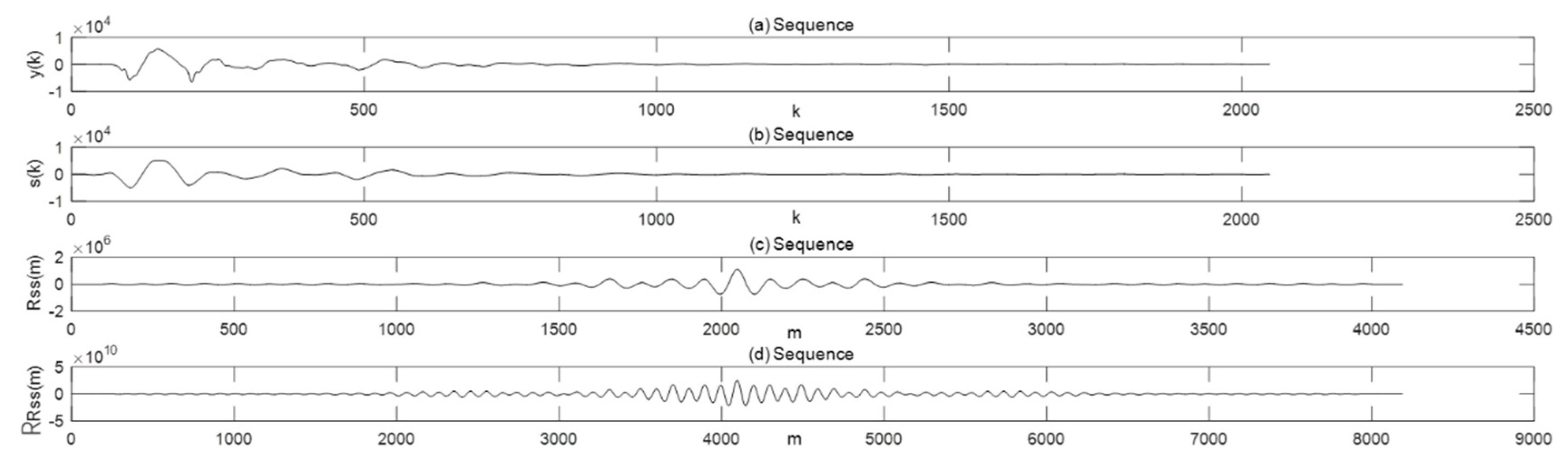
Experimental results with a burial depth of 0.40 m for the buried metal piles with a design length of 1.00 m are selected for display. Figure 4a shows the original sequence waveform of the reflected wave, and Figure 4b depicts the waveform after the wavelet denoising, which is smoother than the original waveform. Figure 4c,d display the waveforms after the first and quadratic self-correlation analysis, respectively. As it can be seen, each subsequent iteration of the analysis highlights the periodicity of the reflected wave. The time–frequency analysis of the signal after quadratic self-correlation analysis is displayed in Figure 5, from which the periodic variation of energy can be seen. Since the data are subjected to self-correlation and STFT, the time–frequency spectrogram is symmetric on the time and frequency axes. The area marked with a black dotted box on the time–frequency spectrogram is selected as the region of interest (ROI). The ROI, which includes the first few complete, regular cycles of the time–frequency spectrogram, is regarded as an object of image processing. At present, the time interval of the ROI is $\Delta =0.008\hspace{0.17em}\hspace{0.17em}\mathrm{s}$, and the pixel columns of the ROI are 420.

The X-direction edge detection is performed on the time–frequency spectrogram using the Sobel operator to obtain an edge image, as shown in Figure 6a. In addition to the obvious pixel periodic distribution, the edge image also contains small textures that need to be removed to reduce the signal obstruction. The edge image is grayed out using the maximum value method, and the gray image with the highest brightness is rendered, as shown in Figure 6b. Figure 6c shows the result of the binarization. Compared to Figure 6b, there are fewer fine textures in Figure 6c. Figure 7a is a statistical waveform of the mean value of the column pixels in the binary image. Although some larger peaks can be seen, the waveform is still hard to interpret. Figure 7b shows the self-correlation operation result of the statistical waveform, with a more defined periodicity. Figure 7c is a spectrum diagram after FFT; the frequency corresponding to the maximum amplitude is 39 Hz (except the zero frequency). The maximum frequency of the signal is 420 Hz. The wave velocity in the buried metal piles is 4800 m/s. The period of the reflected signal is obtained by using Equation (6), and according to Equation (7), the approximate length of the buried metal piles is calculated to be 0.9846 m, with an error of 1.54% for the true length of 1.000 m.

Table 4. Test results of the different depths of the 1.00 m buried metal piles.

Test No.	Calculated Length (m)	Error Rate (%)	Average Error Rate (%)
1	1.0101	1.01	1.10
2	0.9892	1.08
3	0.9899	1.01
4	0.9880	1.20
5	0.9846	1.54
6	0.9900	1.00
7	1.0092	0.92

lists the test results for the different depths of the 1.00 m buried metal piles. Among them, 15 sets of data were collected for each working condition and the values averaged to obtain the measured length. The error range fluctuated between 0.92% and 1.54%, with an average error of 1.10%.

3.3.2. Buried Metal Piles with a Length of 2.00 m

Experimental results of the buried metal piles with a design length of 2.00 m, with a burial depth of 1.20 m, are selected for display in Figure 8. Figure 8a shows the original sequence waveform of the reflected stress wave. Figure 8b shows the waveform after wavelet denoising. Figure 8c,d show first and quadratic self-correlation analysis, respectively. A time–frequency spectrogram is shown in Figure 9 by performing STFT on the signal after multiple iterations of self-correlation operations. The area marked as a black dotted box on the time–frequency spectrogram is selected as the region of interest. The time interval of the ROI region is $\Delta =0.008s$, and the number of columns of the ROI is 420.

Edge detection of the target image in the X direction is performed using the Sobel operator to obtain an edge image, as shown in Figure 10a. Figure 10b shows an image obtained by gradation of the maximum value method, and binarized to obtain Figure 10c. Figure 11a is a statistical waveform of the column pixel mean value in the binary image, and Figure 11b is obtained after the self-correlation operation. FFT is performed in Figure 11c, and the dominant frequency is obtained to be 19 Hz. Bringing $\mathrm{F}=19\hspace{0.17em}\hspace{0.17em}\mathrm{Hz}$ into Equation (6) to obtain the time interval between the reflected signal and the direct signal, and then according to Equation (7), the approximate length of the buried metal piles are calculated to be 2.021 m with an error of 1.05% from the true length of 2.000 m.

Table 5. Different depth test results of the 2.00 m buried metal piles.

Test No.	Calculated Length (m)	Error Rate (%)	Average Error Rate (%)
1	1.9896	0.52	0.70
2	1.9880	0.60
3	2.0127	0.63
4	1.9864	0.68
5	2.0191	0.95
6	1.9900	0.50
7	2.0210	1.05
8	1.9868	0.66

lists the test results for different depths of the 2.00 m buried metal piles. Among them, 15 sets of data were collected for each working condition, and the average value was obtained to obtain the measured length. The depth of the buried metal piles has little effect on the extraction length. The error range fluctuates between 0.50% and 1.05%, and the average error is 0.70%.

3.4. Result Discussion

In Table 4 and Table 5, the error between the measured length and the actual length is less than 2.5 cm, and the average relative error is also within 1.1%, which meets the actual requirements of the project. No direct relationship between the burial depth of the metal pile and the error rate is found in the column “Error rate” in both tables. However, the “average error rate” decreases as the length of the buried metal pile increases, which is consistent with the common sense that relative error will decrease when the base is larger. Compared with existing methods of extracting the stress wave reflection wave period, this algorithm comprehensively utilizes the time–frequency domain information of the signal. The method based on image processing and time–frequency analysis makes the signal interpretation more intuitive, and it can be widely applied in different fields.

The algorithm has the following three advantages: (1) it makes full use of the time–frequency domain information with high accuracy; (2) the fully automatic processing algorithm makes the calculation results unaffected by human factors; and (3) the visual processing process will definitely bring a better experience to users. However, the proposed new algorithm may need big storage to store the measurement data and high computational power to perform FFT and image processing. These common issues of time–frequency analysis can be easily overcome by using recent computer systems. In future work, the algorithm will be simplified and transplanted into an embedded system to promote the algorithm for field tests.

4. Conclusions

This paper proposed a method of extracting the stress wave reflection period based on image processing, and was applied to the length detection of buried metal piles. In the experiments, the vibration hammer was used to strike the buried pile and the stress wave reflection signal was received by a PZT sensor. The time–frequency spectrogram of the reflected signal was obtained after applying wavelet transformation, quadratic self-correlation, and STFT operations. The trough distribution map of the reflection signal was obtained by performing edge detection and image binarization on the time–frequency spectrogram. The valley distribution curve was obtained by calculating the mean value of the column pixels. The curve was processed using FFT and the main frequency was calculated. The reflected wave was then calculated based on the main frequency. Finally, taking the reflection period into the formula for estimating the wave reflection distance, the length of the metal buried pile was calculated. The experiments validated the effectiveness and accuracy of the proposed new algorithm. The average relative error is within 1.1% based on measuring the different lengths of two buried metal piles in the soil. This average relative error can meet the accuracy requirement in industry applications. In addition, the concept of transforming signals into time–frequency domains and analyzing them through image processing has promising applications for health monitoring of other structures.