Heterogeneous Defect Prediction Based on Transfer Learning to Handle Extreme Imbalance

Abstract

Software systems are now ubiquitous and are used every day for automation purposes in personal and enterprise applications; they are also essential to many safety-critical and mission-critical systems, e.g., air traffic control systems, autonomous cars, and Supervisory Control And Data Acquisition (SCADA) systems. With the availability of massive storage capabilities, high speed Internet, and the advent of Internet of Things devices, modern software systems are growing in both size and complexity. Maintaining a high quality of such complex systems while manually keeping the error rate at a minimum is a challenge. This paper proposed a heterogeneous defect prediction method considering class extreme imbalance problem in real software datasets. In the first stage, Sampling with the Majority method (SWIM) based on Mahalanobis Distance is used to balance the dataset to reduce the influence of minority samples in defect data. Due to the negative impact of uncorrelated features on the classification algorithm, the second stage uses ensemble learning and joint similarity measurement to select the most relevant and representative features between the source project and the target project. The third phase realizes the transfer learning from the source project to the target project in the Grassmann manifold space. Our experiments, conducted using nine projects of three public domain software defect libraries and compared with four existing advanced methods to verify the effectiveness of the proposed method in this paper. The experimental results indicate that the proposed method is more accurate in terms of Area under curve (AUC).

1. Introduction

Software defect prediction (SDP) is important to identify defects in the early phases of software development life cycle [1,2]. This early identification, and thereby removal of software defects, is crucial to yield a cost-effective and good quality software product. It usually focuses on estimating the defect proneness of software modules, and helps software practitioners allocate limited testing resources to those parts which are most likely to contain defects. This effort is particularly useful when the whole software system is too large to be tested exhaustively or the project budget is limited.

Software defect datasets are typically characterized by an imbalanced class distribution where the defective samples are fewer than the non-defective samples [3]. The quality of data is usually the most critical factor to determine the performance of a classification model. The class imbalance of defect datasets will seriously affect the prediction performance, especially for extreme imbalance data classification. The prediction model will pay more attention to the non-defect samples, which makes the prediction model more inclined to the non-defect samples, and ignores the cost of error identification of the defective samples. Although the misclassification of defective samples does not significantly reduce the global classification accuracy, the accuracy of defective samples will decline, which is inconsistent with the goal of software defect prediction. Zhou et al. proposed a model which combined attribute selection, sampling technologies and ensemble algorithm to solve the class imbalance problem [4]. Huda et al. introduced a new mixed sampling strategy to generate more pseudo samples from defective classes, and combined random oversampling, Majority Weighted Minority Oversampling Technique, and Fuzzy-Based Feature-Instance Recovery to construct an integrated classifier [5]. It was proven that the prediction performance of Heterogeneous Defect Prediction (HDP) can be improved by balancing defect dataset.

At present, the research on SDP is mainly based on the defect prediction of homogeneous projects, which uses historical data of other projects to construct prediction model. The historical data have the same metrics as the target project, but they are distributed differently. Sufficient historical data are provided for the project to be predicted. However, the programming languages and application fields of different projects are often different, and the corresponding features and distribution are various. It is very difficult to construct a model with homogeneous defect prediction method to have good prediction performance. Therefore, how to use the historical data of other heterogeneous projects to establish a prediction model and predict whether the target project module contains defects, is a research hotspot in the field of software defect prediction.

HDP uses the data of other projects with different measurement standards to realize the defect tendency prediction of the target project. However, due to the different measurement standards and data differences between projects, it cannot be directly used for model construction. Turhan et al. increased the data similarity between different projects by taking advantage of the common features of source and target projects [6]. Nam and Kim et al. used feature selection and feature matching to build the predictor with heterogeneous projects [7]. Jing et al., who combined Unified Metric Representation (UMR) and Canonical Correlation Analysis (CCA), proposed CAA+ to make the distributions of source and target projects similar [8]. However, these methods have three limitations. Firstly, the discarded features may contain the discrimination information of constructing the classification model. Secondly, if the number of common features is less, there may not be enough useful information for accurate prediction. Thirdly, heterogeneous projects may not have common features.

Researchers began to focus on the common potential space between the source project and the target project to settle a matter of great difference in features between heterogeneous projects. Li et al. mapped the source project and the target project to the high-dimensional kernel space, and reduced the difference of data distribution through kernel correlation alignment method [9]. Xu et al. embedded the data from the two domains into a comparable feature space with a low dimensional, measures the difference between the two mapped domains of data using the dictionaries learned from them with the dictionary learning technique [10]. Xu et al. used the spectrum embedding to map the source project and the target project from the high-dimensional space to the low-dimensional consistent space [11].

Transfer learning is introduced into HDP to reduce the problem of data difference, which no longer requires two projects have the same feature dimension and distribution. Transfer learning is an important branch of machine learning. Its goal is to learn knowledge from an existing domain to solve a different but related domain problem. There are three aspects different from traditional machine learning: (1) training and test data can be subject to different distribution. (2) Sufficient labeled data is not required. (3) The model can be transferred between different tasks. It can be used to construct an HDP model with good effect.

However, not all the features can improve the transfer effect in the source project. Only the features contain important information and similar to the distribution of the target project, which are conducive to the construction of a good HDP model. The researchers focused on data processing before transfer learning. Yu et al. achieve feature transfer from the source project to the target project by designing a feature matching algorithm to convert the heterogeneous features into the matched features according to the ‘distance’ of different distributing curves [12]. Ma et al. proposed Kernel Canonical Correlation Analysis based transfer learning algorithm to improve the adaptive ability of prediction model [13]. Wen et al. adopted feature selection and source selection strategies, combined with Transfer Component Analysis to get better prediction performance [14]. Chen et al. proposed a new heterogeneous transfer learning method based on neural network [15]. The instances were transferred to generate quasi real instances. The high credibility quasi real instances were selected to expand the target project data and construct the prediction model. Tong et al. found a series of potential common kernel feature subspaces of source project and target project by combining kernel spectral embedding, transfer learning, and ensemble learning [16]. The above approaches fully proved that the combination of feature selection and feature transferring can improve the performance of an HDP model.

In this paper, the main idea of the proposed approach is to generate samples from the density curve and balance the dataset. It not only reduces the influence of imbalanced data on the classification surface, but also avoids the generation of new samples in the dense area of non-defect samples. Ensemble learning selects some data and establishes multiple Classification and Regression Trees (CART) [17]. The dimensionality reduction of nonlinear data in manifold space can well maintain the complete information of complex structure high-dimensional data, and the inverse mapping of low-dimensional data can also maintain most of the data information [18]. The distortion and deformation of the local feature neighborhood can be reduced by transfer learning in the manifold space. The proposed approach is called Grassmann manifold optimal transfer defect prediction (GMOTDP). A new sample is generated according to the relative density curve of the defective samples of the source project, which can balance the dataset. The optimal subset of source project is constructed by combining with the importance ordering. Joint similarity measurement is used to construct the optimal subset of the target project. Transfer learning in the manifold space is realized by using the optimal subsets of source and target projects. Its main contributions are as follows:

• A new sample data is generated to balance source project. According to the hyperellipticity density curve of the defective samples.
• Use ensemble learning and joint similarity measure to obtain the optimal subsets of source project and target project, respectively.
• Map the non-linear data to Grassmann manifold space, and geodesic flow kernel (GFK) is used to transfer the source project to the same distribution space of the target project.

2. Proposed Framework

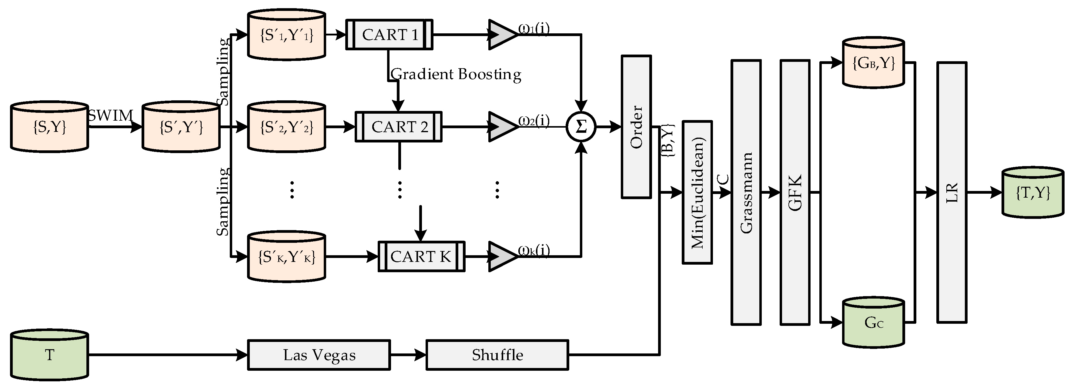
The proposed approach framework of GMOTDP is shown in Figure 1. The algorithm implementation includes the following three parts.

(1) In the oversampling phase, Sampling With the Majority (SWIM) is used to generate new samples along the hyperelliptically dense contour of each defective sample, which is helpful to overcome the limitation of SMOTE, that is, to generate samples outside the convex hull formed by defective samples, and prevents them from being generated in higher probability areas of the non-defect class. Imbalanced source project {S,Y} are oversampled to obtain a balanced dataset {S‘,Y‘}.

(2) In the feature selection phase, the irrelevant features of the source project are firstly removed. The importance of each feature is quantified by using Classification and Regression Tree (CART). The ensemble learning is adopted. The gradient boosting algorithm is used to reduce the loss of CART, and a new tree structure model is generated to ensure the reliability of the final decision. The weighted average of different features in all trees determines the optimal subset of source project to be transferred. For the objective function, the complexity of the tree model is added to the regular term to avoid over fitting. The loss function is expanded by Taylor expansion, and the first derivative and the second derivative are used to quickly optimize the objective. Get the optimal subset of the source project through integration learning. Within a specified number of times, the features of the target project are randomly sorted. By calculating the Euclidean distance of the optimal subset of source projects to determine the similarity, the optimal subset $C$ of the target project to be transferred is jointly determined.

(3) In the feature transferring phase, the traditional Euclidean space measurement is difficult to be used in the real-world nonlinear data; thus, it is necessary to introduce new hypothesis to the data distribution. Manifolds are locally Euclidean spaces, which can find low-dimensional embeddings hidden in high-dimensional data. From the perspective of the topologic, it is locally linear and homeomorphic with low dimensional Euclidean space topology. From the perspective of differential geometry, any tiny part is regarded as Euclidean space. All samples are mapped to the Grassmann manifold. The source project is mapped to the low dimensional common space with the target project G_C by local neighborhood similarity, and the source project {G_B,Y} data similar to the distribution of the target project is obtained with Geodesic Flow Kernel (GFK). Source and target project datasets are inversely mapped. The transformed source project data are trained, and the target project prediction is realized by using Logistic Regression (LR).

2.1. Sampling with the Majority

Generating the samples outside the convex hull formed by the defective samples and preventing them from generating in the dense area of the non-defect samples, SWIM makes full use of the relative distribution information. The Mahalanobis distance (MD) of each given minority class instance corresponds with a hyperelliptical density contour around the majority class, and the minority class is inflated by generating synthetic samples along these contours. New samples are generated along these density curves to expand the defective class. The MD of a sample x from the mean $\overline{\mu }$ is calculated by the inverse matrix ${\overline{\mathrm{\Sigma }}}^{-1}$ of covariance $\overline{\mathrm{\Sigma }}$ as:

$$MD\left(x,\overline{\mu }\right)={\left(x-\overline{\mu }\right)}^T{\overline{\mathrm{\Sigma }}}^{-1}\left(x-\overline{\mu }\right)$$

(1)

Centering the data simplifies the calculation of the distances; this will be evident in a following step, when we generate a new sample point. The mean vector ${\mu }_a$ of the defect free samples is calculated, and the defect free samples $A$ and $B$ are centralized, respectively.

$$A=A-{\mu }_a$$

(2)

$$B=B-{\mu }_a$$

(3)

The MD is equivalent to the Euclidean distance in the whitened space of a distribution. Thus, we simplify the calculations for generating samples by whitening the space. Let $\mathrm{\Sigma }$ denote the covariance matrix of A, we whiten the centered minority class as:

$$B_w=\left(B-{\mu }_a\right){\mathrm{\Sigma }}^{-\frac{1}{2}}$$

(4)

Select a defective sample as the reference datum randomly, generate samples that are at the same Euclidean distance from the mean of the defective class. For each feature $f$ in B_w, we find its mean ${\mu }_f$ and standard deviation ${\sigma }_f$. The bounds of each feature are a random number between ${\mu }_f$ and $l_f$. $\alpha$ controls the number of standard deviations we want the bounds to be. An upper and lower bound on its value, ${\mu }_f$ and $l_f$, as follows:

$${\mu }_f={\mu }_f+\alpha {\sigma }_f$$

(5)

$$l_f={\mu }_f-\alpha {\sigma }_f$$

(6)

Center the data, this implies that the new sample will have the same Euclidean norm as the defective sample. We transform $z$ as:

$$z_{norm}=z\frac{{\left|\right|x\left|\right|}_2}{{\left|\right|S\left|\right|}_2}$$

(7)

Transform each new sample to the original space, where the new sample $z_{new}$ will be in the same density curve as the reference datum:

$$z_{new}={\left({\mathrm{\Sigma }}^{-\frac{1}{2}}\right)}^{-1}{z}_{norm}$$

(8)

This process can be repeated t times, where t is the desired number of samples to be generated based on the reference datum. SWIM is summarized as in Algorithm 1.

Algorithm 1. Sampling with the Majority

Input: imbalanced and labeled source dataset S, Sampling rate $\alpha$. Output: balanced and labeled source dataset $S_{new}$. Method: N = number of samples (undefect class $A-$ defected class $B$). Compute ${\mu }_a$ and covariance matrix $\mathrm{\Sigma }$ with. Whiten $B$ as $B_w=\left(B-{\mu }_a\right){\mathrm{\Sigma }}^{-\frac{1}{2}}$, compute mean ${\mu }_f$ and standard deviation ${\sigma }_f$ for each feature $f$. fori = 1 to t, $t=\alpha \times N$ do select a sample $x$ randomly from $B$. Generate new sample $z$, each feature $z_f$ is $\left({\mu }_f+\alpha {\sigma }_f\right)\le z_f\le \left({\mu }_f-\alpha {\sigma }_f\right)$. transform s back into original space, $z_{new}={\left({\mathrm{\Sigma }}^{-\frac{1}{2}}\right)}^{-1}z\frac{{\left|\right|x\left|\right|}_2}{{\left|\right|S\left|\right|}_2}$ end for return$S_{new}$

In order to verify the effectiveness of SWIM and produce representative results, an imbalanced training set with 10 minority samples and 88 majority samples and a balanced test set with 300 samples are created. The demonstration is presented in Figure 2. The left figure shows the results of oversampling using SWIM with an imbalanced dataset. The right figure shows the classification results of the support vector machine without oversampling. The majority class training samples are shown as red squares with black outlines, and the corresponding test samples are shown as red circles. The minority class training samples are shown as blue squares with white outlines, and the corresponding test samples are shown as blue circles. The new samples by SWIM are shown as cyan squares with white outlines. It can be seen from the Figure 1 that the samples generated by SWIM are spread along the density curve corresponding of the minority data from the majority class. From the decision surfaces generated by the two classifiers (represented by the shading in the plot), it can be seen that using the information in majority class to generate samples can lead more representative decision surface, which obtains better classification performance.

In order to prove the effectiveness of this method, the classification results of the training set without sampling and SWIM are calculated. We divided a defect dataset into a training set and test set with a ratio of 7:3, which is classified by SVM. The average results of 10 times are shown in

Table 1. AUC obtained by using SVM without sampling (Baseline), and with SWIM.

Project	Baseline	SWIM
PC3	0.7792	0.8293
PC4	0.7398	0.8231
MW1	0.8229	0.8678
EQ	0.7948	0.8730
JDT	0.9219	0.9633
LC	0.8011	0.8658
AR3	0.8472	0.8666
AR4	0.9587	0.9892
AR5	0.8752	0.9375

. It shows that SWIM has a significant advantage when the relative and absolute imbalance is very high.

2.2. Feature Selection

This phase selects the optimal subset of the source and target projects for feature transfer. Quantify the importance of each feature to select features by using the tree model. In the process of CART construction, select the feature with the maximum gain to segment to the maximum depth, and achieve the minimum cost of CART segmentation. When constructing the next tree using the ensemble learning, the objective function adds complexity. The first and the second derivatives are used to reduce the loss of cart, minimize the objective function and ensure the reliability of the final decision. All features of all trees are weighted and averaged to determine their importance.

During the construction of cart, the idea of minimizing the objective function is as follows:

$$L_k={\displaystyle \sum }_i^{n}l\left(y_i,{\widehat{y}}_i\right)+{\displaystyle \sum }_k\mathsf{\Omega }\left(p_k\right)$$

(9)

$$\mathsf{\Omega }\left(p\right)=\gamma T+\frac{1}{2}\lambda {\left|\right|\omega \left|\right|}^2$$

(10)

Here, $l$ is a differentiable convex loss function, which is used to measure the difference between the prediction ${\widehat{y}}_i$ and the target $y_i$. The second term $\mathsf{\Omega }$ penalizes the complexity of the model, which helps to smooth the final learning weights to avoid over-fitting. $T$ is the number of leaf nodes, $\left|\right|\omega \left|\right|$ is the magnitude of leaf node vector, $\gamma$ represents the difficulty of sharding a node, and $\lambda$ represents the L2 regularization coefficient.

$$L_k={\displaystyle \sum }_i^{n}l\left(y_i,{\widehat{y}}_{i\left(k-1\right)}+p_k\left(x_i\right)\right)+\mathsf{\Omega }\left(p_k\right)$$

(11)

$$p_k\left(x_i\right)={\omega }_{q\left(x_i\right)}$$

(12)

where ${\widehat{y}}_{i\left(k\right)}$ is the prediction of the $i$-th sample at the $k$-th iteration. $q\left(x_i\right)$ is the structure function of each tree that maps an example to the corresponding leaf index. The objective function greedily adds $p_k\left(x_i\right)$. Each $p_k\left(x_i\right)$ corresponds to an independent tree structure $q\left(x_i\right)$ and leaf weights $w$.

$$L_k={\displaystyle \sum }_{i=1}^n\left[l\left(y_i,{\widehat{y}}_{i\left(k-1\right)}\right)+g_i{p}_k+\frac{1}{2}{h}_i{p}_k^2\right]+\mathsf{\Omega }\left(p_k\right)$$

(13)

Second-Order approximation optimizes the target quickly, where $g_i={\partial }_{{\widehat{y}}_{i\left(k-1\right)}}l\left(y_i,{\widehat{y}}_{i\left(k-1\right)}\right)$ and $h_i={\partial }_{{\widehat{y}}_{i\left(k-1\right)}}^{2}l\left(y_i,{\widehat{y}}_{i\left(k-1\right)}\right)$ are the first and the second order gradient statistics of the loss function, and removes the constant term of the objective function.

$$\begin{array}{c}{L}_k={\displaystyle \sum }_i^{n}l\left(y_i,{\widehat{y}}_{i\left(k-1\right)}+p_k\right)+\mathsf{\Omega }\left(p_k\right)\\ ={\displaystyle \sum }_i^{n}l\left(y_i,{\widehat{y}}_{i\left(k-1\right)}+p_k\right)+\gamma T+\frac{1}{2}\lambda {\displaystyle \sum }_{j=1}^T{w}_j^2\\ ={{\displaystyle \sum }}_{j=1}^T\left[\left({{\displaystyle \sum }}_{i\in I_j}^{}{g}_i\right){\omega }_j+\frac{1}{2}\left({{\displaystyle \sum }}_{i\in I_j}^{}{h}_i+\lambda \right){\omega }_j^2\right]+\mathsf{\gamma }\mathrm{T}\end{array}$$

(14)

The weight $w_j$ of each leaf in each tree is obtained, which is used to calculate the feature importance:

$$w_j=-\frac{{{\displaystyle \sum }}_{i\in I_j}{g}_i}{{{\displaystyle \sum }}_{i\in I_j}{h}_i+\lambda }$$

(15)

Las Vegas is a typical randomization method, namely, one of probability algorithms. It has the characteristics of probability algorithm, which allows the algorithm to randomly select the next step in the process of execution. In many cases, when the algorithm is faced with a choice in the process of execution, the randomness choice spends less time than the optimal choice, thus, the probability algorithm can greatly reduce the complexity of the algorithm. In this paper, Las Vegas is used to randomly sort the features of the target project, and calculate the Euclidean distance with the source project to measure the similarity. In a certain number of times, the subset with the highest distribution similarity is selected as the optimal subset of the target project for subsequent transfer learning. Feature selection is summarized as in Algorithm 2.

Algorithm 2. Feature Selection

1. Input: feature $f\left(i\right)\in S_{new}$, label $y\left(i\right)\in S_{new}$, $i=1\cdots n$, the number and depth of CART $K$, $D$. imbalanced and unlabeled source dataset $X_T$, random number R Output: Similar dataset $X_{S-sim}$, $X_{T-sim}$ Method: 2. for k = 1 to K, do 3. for d = 1 to D, do 4. sampling($S_{new}\times 0.4$) 5. $f_i$→$\left(gain\left(f_i\right)\right)$ 6. select $maxGain\left(f_i\right)$ to split 7. end for 8. prediction label: ${\widehat{y}}_i$, complex index: $p_k$, feature weight, $\omega \left(f_i\right)$ 9. $L_k={\displaystyle \sum }_i^{n}l\left(y_i,{\widehat{y}}_{i\left(k-1\right)}+p_k\right)+\mathsf{\Omega }\left(p_k\right)$ 10. second-order approximation $L_k={\displaystyle \sum }_{i=1}^n\left[g_i{p}_k+\frac{1}{2}{h}_i{p}_k^2\right]+\mathsf{\Omega }\left(p_k\right)$ 11. $g_i={\partial }_{{\widehat{y}}_{i\left(k-1\right)}}l\left(y_i,{\widehat{y}}_{i\left(k-1\right)}\right)$, $h_i={\partial }_{{\widehat{y}}_{i\left(k-1\right)}}^{2}l\left(y_i,{\widehat{y}}_{i\left(k-1\right)}\right)$. 12. end for 13. avg(${\omega }_k(f_i)$, $w_j(k)$)→sort($f_i$)→$S_{imp}$ 14. for r = 1 to $R$, do 15. shuffle($X_T,col$) 16. select dataset $X_{T-rand}$, col($X_{T-rand}$) = col($X_{S-imp}$) 17. euclidean($X_{T-rand}$, $X_{S-imp}$) 18. end for 19. $X_{S-sim}$, $X_{T-sim}$ by min(euclidean($X_{T-rand}$, $X_{S-imp}$))

2.3. Transfer Learning in Manifold Space

Manifold is homeomorphic spaces in local and Euclidean spaces. It uses Euclidean distance to calculate the distance, which overcomes the feature distortion of transfer learning in original space. The Grassmann manifold can take the original d-dimensional subspace as the basic element to help learning classifier. It usually has an effective numerical form in feature transformation, which can be very efficient representation and solution in the transfer learning problem. In addition, the transfer of source project to target project, or the transfer of source and target projects to a common space are two main methods of feature-based transfer learning. Li et al. found that the performance of the transfer of source project to target project is better than the latter [19]. In this paper, the optimal subset of source and target projects are transformed into the Grassmann manifold. Geodesic Flow Kernel (GFK) method is used to construct geodesic flow to make the source domain close to the target domain. It integrates the space function of the manifold where these two points are located of the source project with the same distribution as the target project is obtained.

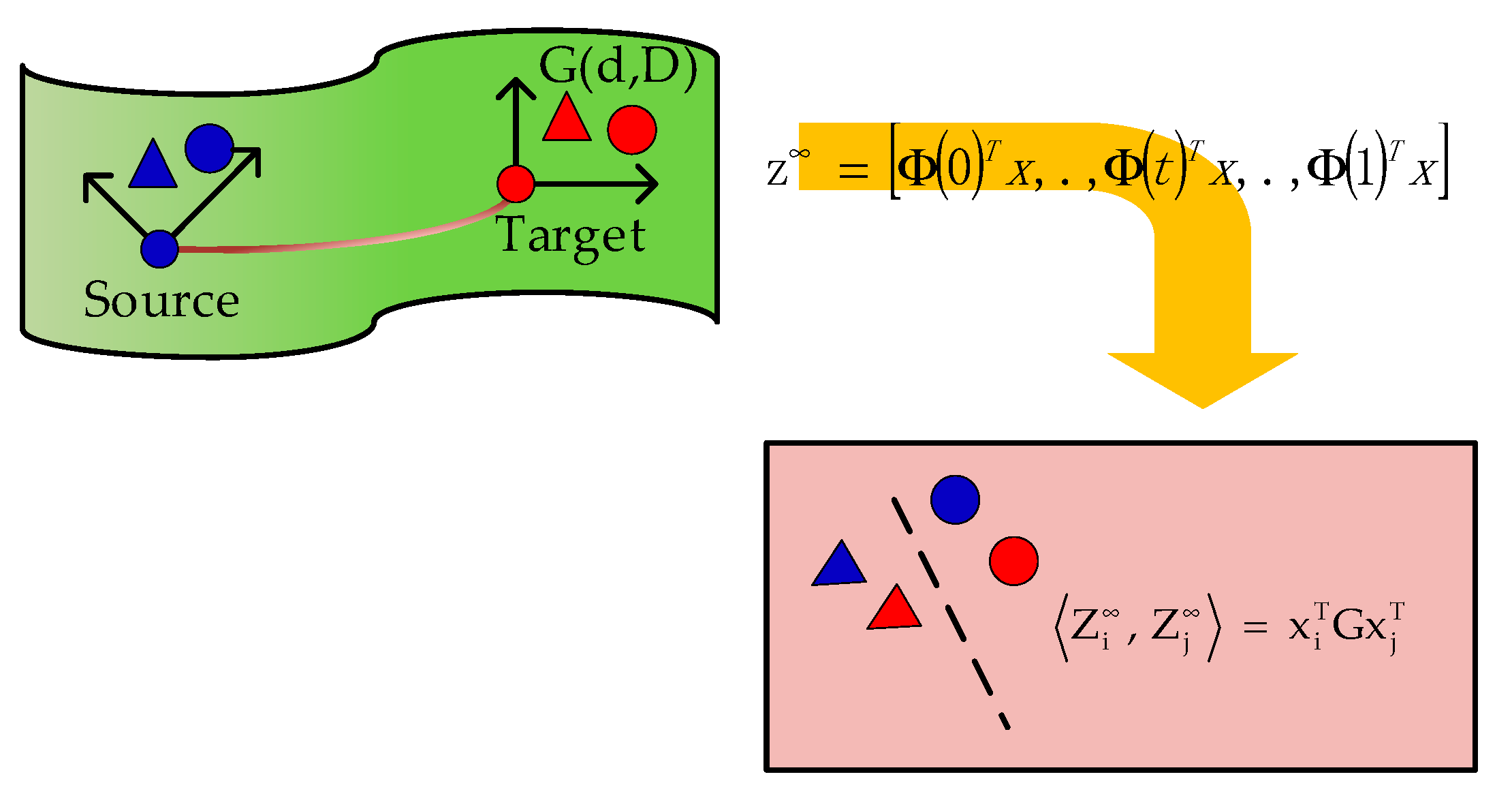
As shown in the Figure 3, GFK tries to embed the $D\times d$ dimension subspace $P_s$, $P_T\in R^{D\times d}$ after dimensionless reduction of the source domain and target domain into the manifold G. $\varphi \left(0\right)$ is the source domain representation of manifold G, $\varphi \left(1\right)$ is the target domain representation of manifold G, and the geodesic flow between $\varphi \left(0\right)$ and $\varphi \left(1\right)$ is equivalent to transforming the original feature space into an infinite dimension space, reducing the drift phenomenon between domains. The parameterization is shown as follows:

$$\begin{array}{c}\mathsf{\Phi }:t\in \left[0,1\right]\to \mathsf{\Phi }:t\in G\left(d,D\right)\\ P_S=\mathsf{\Phi }\left(0\right),P_T=\mathsf{\Phi }\left(1\right)\end{array}$$

(16)

$\mathsf{\Phi }\left(t\right)$ is represented as follows, where $U_1$, $U_2$ are orthogonal matrices obtained by SVD.

$$\mathsf{\Phi }\left(t\right)=P_S{U}_1\mathrm{\Gamma }\left(t\right)-R_S{U}_2\mathrm{\Sigma }\left(t\right)$$

(17)

$$P_S^T{P}_T=U_1\mathrm{\Gamma }\left(t\right)V^T,R_S^T{P}_T=-U_2\mathrm{\Sigma }\left(t\right)V^T$$

(18)

$z^{\infty }=\left[\mathsf{\Phi }{\left(0\right)}^{T}x,\dots ,\mathsf{\Phi }{\left(t\right)}^{T}x,\dots ,\mathsf{\Phi }{\left(1\right)}^{T}x\right]$ is the feature of manifold space, the inner product of transformed features gives rise to positive semidefinite geodesic flow kernel:

$$\langle z_i^{\infty },z_j^{\infty }\rangle ={{\displaystyle \int }}_0^1{(\mathsf{\Phi }{\left(t\right)}^T{x}_i)}^T(\mathsf{\Phi }{\left(t\right)}^T{x}_j)dt=x_i^{T}G{x}_j$$

(19)

Thus, the features in the original space can be transformed into the Grassmann manifold with $z=\sqrt{G}x$. G can be effectively calculated by singular value decomposition.

$$G=\left[P_S{U}_1{R}_S{U}_2\right]\left[\begin{array}{cc}{\mathrm{\Lambda }}_1& {\mathrm{\Lambda }}_2\\ {\mathrm{\Lambda }}_2& {\mathrm{\Lambda }}_3\end{array}\right]\left[\begin{array}{c}{U}_1^T{P}_S^T\\ U_2^T{R}_S^T\end{array}\right]$$

(20)

Logistic regression is used as classifier to train the source project with the same distribution as the target project, and use the model to distinguish the defect type of the target item module.

3. Experimental Results and Analysis

3.1. Datasets Description

The experimental data are from three open databases in the field of software defect prediction: NASA [20], AEEEM [21], SOFTLAB [22]. Table 1 lists the details of the datasets used in the experiment. Each dataset represents a software system or subsystem, including the static code indicators and corresponding fault data of each component module. Although these three databases have different number of features, some databases have common features.

Table 2. Details of projects used in the comparison experiments.

Company	Project	Language	Description	Metrics	Instance	Defective (%)
NASA	PC3	C	Flight Software for Each Orbiting Satellite	37	1077	134 (12.44%)
	PC4	C	Flight Software for Each Orbiting Satellite	37	1458	178 (12.21%)
	MW1	C	A Zero Gravity Experiment about Combustion	37	253	27 (10.67%)
AEEEM	EQ	Java	OSGi Framework	61	324	129 (39.81%)
	JDT	Java	IDE Development	61	997	206 (20.66%)
	LC	Java	Text Search Engine Library	61	691	64 (9.26%)
SOFTLAB	AR3	C	Embedded Controller of The Washing Machine	29	63	8 (12.7%)
	AR4	C	Embedded Controller of The Dishwasher	29	107	20 (18.69%)
	AR5	C	Embedded Controller of The Refrigerator	29	36	8 (22.22%)

shows the situation of common features between databases. NASA comes from NASA’s space system related software, which is written in C language. Its features include the number of lines of code, software complexity, and software readability. AEEEM is collected by D’Ambros and written in Java language. Its features include change entropy measurement and source code measurement. SOFTLAB comes from Turkish software company and is written in C language. Both SOFTLAB and NASA used in the experiments are obtained from PROMISE [22], and there are 28 common features between them. There are redundant samples and features in NASA, and we choose the clean-up version NASA MDP. Projects of MW1 and LC, and so on, are all extreme imbalance datasets.

3.2. Experimental Results

Experiments used the Bob under Linux as the backend. Python the multi-paradigm programming language with rich data science packages has been selected. The information of hardware is CPU: Intel^® Core™ i7-9750H, Video card: NVIDIA Geforce RTX 2060.

In order to investigate the performance of the proposed algorithm in this paper, GMOTDP is compared with the existing state-of-the-art defect prediction methods, such as TCA+ [23], CCA+ [8], KCAA+ [13], and KSETE [16]. TCA+ and CCA+ are benchmark comparison methods for heterogeneous defect prediction. KCAA+ and KSETE are new heterogeneous defect prediction methods in 2017 and 2019. All methods use logistic regression as the classifier. In the experiments, one project was selected as the target project, and the projects in different datasets were used as the source project for heterogeneous prediction. The area under the working characteristic curve (AUC) of the subjects was used as the evaluation index of the prediction model. The value of AUC ranged from 0 to 1, which is larger, the classification effect of the model is better. For example, six forecasting cases can be carried out for a given SOFTLAB database, when AR3 is selected as the target project. They are called PC3 ≥ AR3, PC4 ≥ AR3, MW1 ≥ AR3, EQ ≥ AR3, JDT ≥ AR3, LC ≥ AR3. Because GMOTDP involves randomness when dealing with class imbalance and feature selection, the average results of 50 repeated experiments were counted for each case to reduce the influence of randomness on the experimental results.

The number of common features between projects of different companies is shown in

Table 3. The number of common features between projects of different companies.

Company A ∩ Company B	NASA ∩ SOFTLAB	AEEEM ∩ SOFTLAB	NASA ∩ AEEEM
Number	28	0	0

. In this paper, two sets of experiments are designed to verify the predictive performance of GMOTDP, which is not affected by whether the source and target projects have common features or not. When there are common features between two projects, the projects of NASA and SOFTLAB are used as the source projects and the target projects, respectively, for comparison experiments. When two projects have not common features, the projects of AEEEM and SOFTLAB are used as the source projects and the target projects, respectively, for comparison experiments.

Table 4. Mean AUC results for source and target projects with common features using different methods.

Source	Target	TCA+	CCA+	KCCA+	KSETE	GMOTDP
PC3	AR3	0.6399	0.6232	0.7689	0.7474	0.8297
	AR4	0.7151	0.6462	0.7389	0.7743	0.9014
	AR5	0.6249	0.6692	0.7516	0.8242	0.9330
PC4	AR3	0.6920	0.6769	0.7310	0.7846	0.8079
	AR4	0.6930	0.6462	0.7371	0.7047	0.9252
	AR5	0.7214	0.6492	0.7229	0.7728	0.8460
MW1	AR3	0.6696	0.6464	0.7089	0.6398	0.8170
	AR4	0.6860	0.6923	0.8259	0.7964	0.8682
	AR5	0.6429	0.5462	0.6850	0.8286	0.9397
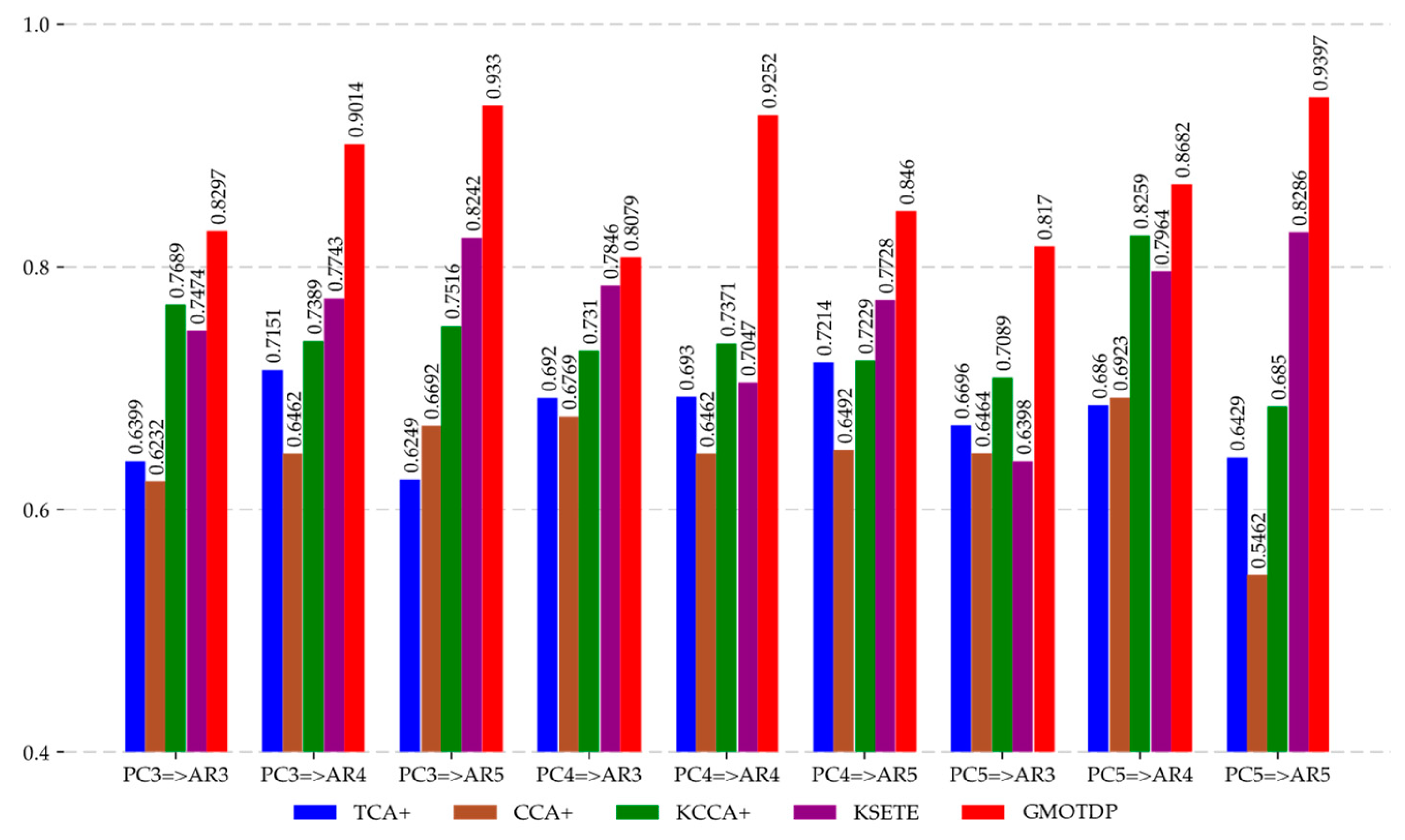
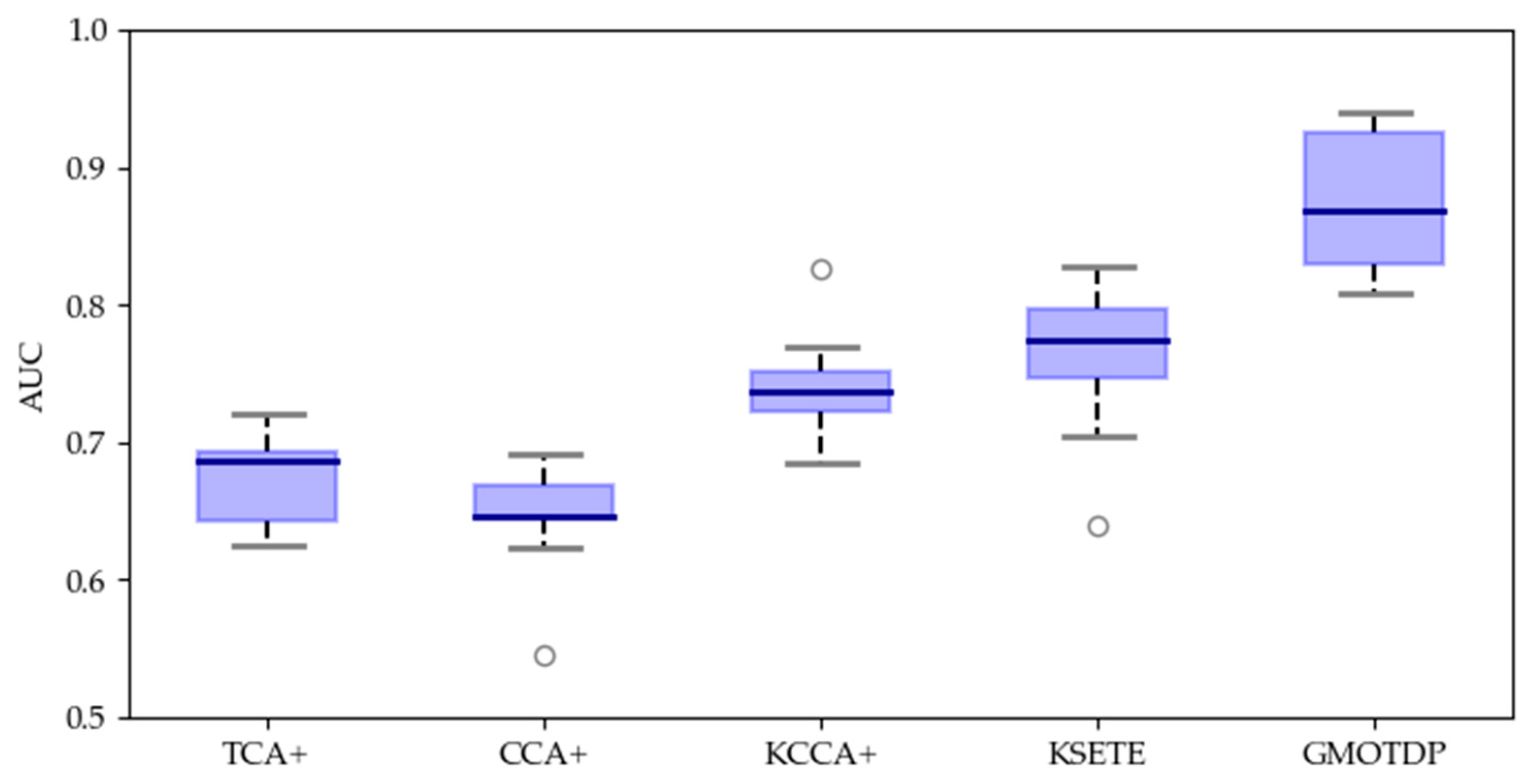
mean		0.6761	0.6437	0.7411	0.7636	0.8742

shows the AUC values of GMOTDP compared with the other four methods when the source and target projects have common features. We selected datasets from NASA and SOFTLAB as source and target projects, respectively. Figure 4 graphically displays Table 4 for a more intuitive display and comparison of the predicted results. It can be seen from Figure 4 and Table 4 that the performance of GMOTDP is better than other methods, and the AUC average value of the prediction results of the other four methods is improved by 0.1981, 0.2305, 0.1331, and 0.1106, respectively. It can be seen that the prediction effect of GMOTDP is better than the other four methods from the boxplot representation of Figure 5.

Table 5. Mean AUC results for source and target projects without common features using different methods.

Source	Target	TCA+	CCA+	KCCA+	KSETE	GMOTDP
EQ	AR3	0.5504	0.5846	0.7043	0.7129	0.8382
	AR4	0.5559	0.6462	0.7784	0.7850	0.9145
	AR5	0.5795	0.6923	0.6830	0.6654	0.9397
JDT	AR3	0.5625	0.5692	0.6572	0.6806	0.8326
	AR4	0.5640	0.6462	0.7528	0.7469	0.9236
	AR5	0.6429	0.5692	0.5931	0.7849	0.7515
LC	AR3	0.5982	0.5846	0.7188	0.7294	0.8065
	AR4	0.5530	0.6077	0.5545	0.7367	0.9031
	AR5	0.5661	0.6154	0.6524	0.7754	0.9115
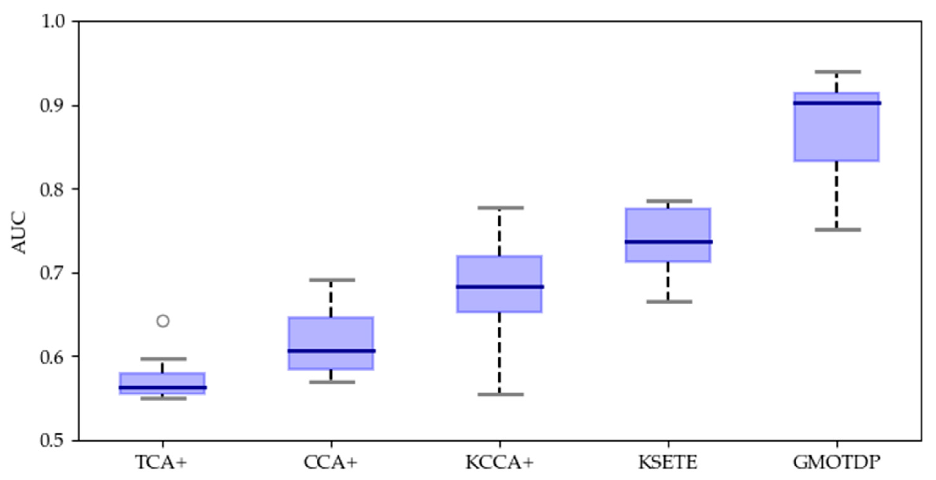
mean		0.5747	0.6093	0.6772	0.7352	0.8690

shows the AUC values of GMOTDP compared with the other four methods when there are no common features between the source project and the target project. We selected datasets from AEEEM and SOFTLAB as source and target projects, respectively. In Figure 6, the results of Table 5 are shown graphically, the various colored columns indicate the same as above. It can be seen from Table 5 and Figure 6, the mean value of GMOTDP is 0.8690, while the mean values of other methods are 0.5747, 0.6093, 0.6772, and 0.7352, respectively. The boxplot representation in Figure 7 shows that the prediction effect of GMOTDP is better than other methods.

When Table 4 and Table 5 are compared, it can be seen that the prediction performance of GMOTDP is not affected by whether there are common features. TCA+, CCA+, and KCCA methods have different degrees of decrease in predictive performance between source and target projects without a common feature. The reason for this situation is that PCA is used to extract the principal components of source and target projects when constructing manifold space, and the reconstructed features can retain most of the relevant information characteristics. GMOTDP does not lose the important information related to defects in data processing, which ensures the effectiveness and universality.

The non-parametric test does not assume that the population distribution must conform to the normal distribution. It can infer that the population distribution directly from samples. The Kruskal-Wallis test is carried out under significance level α = 0.05, and TCA+, CCA+, KCCA+, KSETE, and GMOTDP are compared in pairs. The null hypothesis for each row in

Table 6. Kruskal-Wallis H and Holm-Bonferroni correction.

Method 1	Method 2	p-Value	Holm-Bonferroni Correction
TCA+	CCA+	0.949	1.000
TCA+	KCCA+	0.005	0.054
TCA+	KSETE	<0.001	0.001
TCA+	GMOTDP	<0.001	<0.001
CCA+	KCCA+	0.007	0.066
CCA+	KSETE	<0.001	0.001
CCA+	GMOTDP	<0.001	<0.001
KCCA+	KSETE	0.238	1.000
KCCA+	GMOTDP	<0.001	0.001
KSETE	GMOTDP	0.006	0.064

show that the Method 1 and Method 2 distributions are the same. In order to reveal which of these groups differ from each other, we conduct a post hoc test with the Holm-Bonferroni correction. We use SPSS software to obtain adjusted p-value, which is directly compared with 0.05, and the difference is considered statistically significant if it is less than 0.05. The last column of the Table 6 clearly shows that there is a significant difference between GMOTDP and TCA+, CCA+, and KCCA+, but there is no significant difference between GMOTDP and KSETE.

For the imbalanced datasets, G-mean was used to compare the performance of each prediction method again. $\mathrm{G}-\mathrm{mean}=\sqrt{TNR\times Recall}$,$TNR$ and $Recall$ denotes specificity and sensitivity of the classifier, respectively. G-mean comprehensive considers the classification performance of minority class and majority class. When the classification accuracy of minority class and majority class is closer, we can get the best G-mean value. It can be found from

Table 7. Mean G-mean results for source and target projects with common features using different methods.

Source	Target	TCA+	CCA+	KCCA+	KSETE	GMOTDP
PC3	AR3	0.5835	0.6618	0.7090	0.7129	0.7800
	AR4	0.5796	0.6208	0.6790	0.6924	0.7630
	AR5	0.5909	0.6092	0.5909	0.7334	0.8018
PC4	AR3	0.5998	0.6196	0.7049	0.6882	0.7951
	AR4	0.5043	0.6167	0.6898	0.6764	0.7734
	AR5	0.5797	0.5912	0.6008	0.7369	0.7823
MW1	AR3	0.5687	0.6366	0.6144	0.6939	0.7796
	AR4	0.5454	0.6466	0.6544	0.7206	0.8148
	AR5	0.6891	0.6723	0.6009	0.7341	0.7622
mean		0.5823	0.6305	0.6493	0.7099	0.7836

and

Table 8. Mean G-mean results for source and target projects without common features using different methods.

Source	Target	TCA+	CCA+	KCCA+	KSETE	GMOTDP
EQ	AR3	0.5977	0.6344	0.6593	0.6847	0.7922
	AR4	0.5527	0.5890	0.6096	0.6836	0.7710
	AR5	0.5345	0.6396	0.6793	0.7188	0.7662
JDT	AR3	0.5955	0.6207	0.6269	0.7358	0.8158
	AR4	0.6736	0.6213	0.6096	0.7297	0.7766
	AR5	0.5924	0.6065	0.6669	0.7306	0.7393
LC	AR3	0.5797	0.6355	0.6519	0.7312	0.7834
	AR4	0.6145	0.6044	0.5929	0.7351	0.7710
	AR5	0.5671	0.6421	0.6308	0.7275	0.7902
mean		0.5897	0.6215	0.6363	0.7197	0.7784

that the prediction effect of GMOTDP is better.

4. Conclusions

This paper proposes a three-phase heterogeneous software prediction method-GMOTDP, which includes SWIM oversampling, feature selection and transfer learning. New minority samples are generated to balance the source project dataset based on Mahalanobis distance. CART-based ensemble learning is used to determine the optimal subset of source project. The joint similarity measure is used to obtain the optimal subset of the target project. According to the transfer of optimal subsets in manifold space, the source project with the same distribution as the target project are obtained, which reaches the condition of traditional classification and predicts the defect tendency of the target project module.

A lot of experiments were designed to validate the propose scheme using nine projects of three public domain software defect datasets. Compared with several representative software defect prediction methods, the proposed GMOTDP has better prediction effect. AUC results show that our method performs better usually than other four methods.

In the future, we will study how to combine other supervised learning methods with the sample level and algorithm level methods, and investigate the influence of extreme class imbalance in semi-supervised software defect predictor on more datasets. This is an interesting issue to be explored, which might shed light on the design of more powerful supervised learning algorithms.

References

1. Malhotra, R.; Kamal, S. An Empirical Study to Investigate Oversampling Methods for Improving Software Defect Prediction Using Imbalanced Data. Neurocomputing 2019, 343, 129–140. [Google Scholar] [CrossRef]
2. Ji, H.J.; Huang, S.; Lv, X.W.; Wu, Y.N.; Feng, Y.T. Empirical Studies of a Kernel Density Estimation Based Naive Bayes Method for Software Defect Prediction. IEICE Trans. Inf. Syst. 2019, E102D, 75–84. [Google Scholar] [CrossRef] [Green Version]
3. Bennin, K.E.; Keung, J.W.; Monden, A. On the Relative Value of Data Resampling Approaches for Software Defect Prediction. Empir. Softw. Eng. 2019, 24, 602–636. [Google Scholar] [CrossRef]
4. Zhou, L.J.; Li, R.; Zhang, S.D.; Wang, H. Imbalanced Data Processing Model for Software Defect Prediction. Wirel. Pers. Commun. 2018, 102, 937–950. [Google Scholar] [CrossRef]
5. Huda, S.; Liu, K.; Abdelrazek, M.; Ibrahim, A.; Alyahya, S.; Al-Dossari, H.; Ahmad, S. An Ensemble Oversampling Model for Class Imbalance Problem in Software Defect Prediction. IEEE Access 2019, 23, 9919–9935. [Google Scholar] [CrossRef]
6. Turhan, B.; Menzies, T.; Bener, A.B.; Stefano, J.D. On the Relative Value of Cross-Company and Within-Company Data for Defect Prediction. Empir. Softw. Eng. 2009, 14, 540–578. [Google Scholar] [CrossRef] [Green Version]
7. Nam, J.; Kim, S. Heterogeneous Defect Prediction. In Proceedings of the 2015 10th Joint Meeting on Foundations of Software Engineering, Bergamo, Italy, 30 August–4 September 2015; pp. 508–519. [Google Scholar]
8. Jing, X.Y.; Wu, F.; Dong, X.W.; Qi, F.M.; Xu, B.W. Heterogeneous Cross-Company Defect Prediction by Unified Metric Representation and CCA-Based Transfer Learning. In Proceedings of the 2015 10th Joint Meeting on Foundations of Software Engineering, Bergamo, Italy, 30 August–4 September 2015; pp. 496–507. [Google Scholar]
9. Li, Z.Q.; Jing, X.Y.; Zhu, X.K.; Zhang, H.Y. Heterogeneous Defect Prediction Through Multiple Kernel Learning and Ensemble Learning. In Proceedings of the 2017 IEEE International Conference on Software Maintenance and Evolution (ICSME), Shanghai, China, 17–22 September 2017; pp. 12–22. [Google Scholar]
10. Xu, Z.; Yuan, P.P.; Zhang, T.; Tang, Y.T.; Li, S.; Xia, Z. HDA: Cross-Project Defect Prediction via Heterogeneous Domain Adaptation with Dictionary Learning. IEEE Access 2018, 6, 57597–57613. [Google Scholar] [CrossRef]
11. Xu, Z.; Ye, S.Z.; Zhang, T.; Xia, Z.; Pang, S.; Wang, Y. MVSE: Effort-Aware Heterogeneous Defect Prediction via Multiple-View Spectral Embedding. In Proceedings of the 2019 IEEE 19th International Conference on Software Quality, Reliability and Security (QRS), Sofia, Bulgaria, 22–26 July 2019; pp. 10–17. [Google Scholar]
12. Yu, Q.; Jiang, S.J.; Zhang, Y.M. A Feature Matching and Transfer Approach for Cross-company Defect Prediction. J. Syst. Softw. 2017, 132, 366–378. [Google Scholar] [CrossRef]
13. Ma, Y.; Zhu, S.Z.; Chen, Y.M. Kernel CCA Based Transfer Learning for Software Defect Prediction. IEICE Trans. Inf. Syst. 2017, E100D, 1903–1906. [Google Scholar] [CrossRef] [Green Version]
14. Wen, W.Z.; Zhang, B.; Gu, X.; Ju, X.L. An Empirical Study on Combining Source Selection and Transfer Learning for Cross-Project Defect Prediction. In Proceedings of the 2019 IEEE 1st International Workshop on Intelligent Bug Fixing (IBF), Hangzhou, China, 24 February 2019; pp. 29–38. [Google Scholar]
15. Chen, J.Y.; Yang, Y.T.; Hu, K.K.; Xuan, Q. Multiview Transfer Learning for Software Defect Prediction. IEEE Access 2019, 7, 8901–8916. [Google Scholar] [CrossRef]
16. Tong, H.N.; Liu, B.; Wang, S.H. Kernel Spectral Embedding Transfer Ensemble for Heterogeneous Defect Prediction. IEEE Trans. Softw. Eng. 2019. [Google Scholar] [CrossRef]
17. Chen, T.Q.; Guestrin, C. XGBoost: A Scalable Tree Boosting System. In Proceedings of the 22nd ACM SIGKDD International Conference on Knowledge Discovery and Data Mining, San Francisco, CA, USA, 13–17 August 2016; pp. 785–794. [Google Scholar]
18. Wang, J.; Feng, W.; Chen, Y.; Yu, H.; Huang, M.; Yu, P.S. Visual Domain Adaptation with Manifold Embedded Distribution Alignment. In Proceedings of the 26th ACM international conference on Multimedia, Seoul, Korea, 22–26 October 2018; pp. 402–410. [Google Scholar]
19. Sharma, S.; Bellinger, C.; Krawczyk, B.; Japkowicz, N.; Zaïane, O. Synthetic Oversampling with the Majority Class: A New Perspective on Handling Extreme Imbalance. In Proceedings of the 2018 IEEE International Conference on Data Mining, Singapore, 17–20 November 2018; pp. 447–455. [Google Scholar]
20. Shepperd, M.; Song, Q.; Sun, Z. Data Quality: Some Comments on the NASA Software Defect Datasets. IEEE Trans. Softw. Eng. 2013, 39, 1208–1215. [Google Scholar] [CrossRef] [Green Version]
21. Marco, D.; Michele, L.; Romain, R. An Extensive Comparison of Bug Prediction Approaches. In Proceedings of the IEEE Working Conference on Mining Software Repositories, Cape Town, South Africa, 2–3 May 2010; pp. 31–41. [Google Scholar]
22. Jureczko, M.; Madeyski, L. Towards Identifying Software Project Clusters with Regard to Defect Prediction. In Proceedings of the 6th International Conference on Predictive Models in Software Engineering, Timişoara, Romania, 12–13 September 2010; pp. 1–10. [Google Scholar]
23. Nam, J.; Pan, S.J.; Kim, S. Transfer Defect Learning. In Proceedings of the 2013 35th International Conference on Software Engineering (ICSE), San Francisco, CA, USA, 18–26 May 2013; pp. 382–391. [Google Scholar]
Figure 1. The overall architecture of GMOTDP.
Applsci 10 00396 g001
Figure 2. (a) Shows the binary support vector classifier induced over the imbalanced training set; (b) Shows the illustration of classifier produced by using SWIM.
Applsci 10 00396 g002
Figure 3. Geodesic Flow Kernel.
Applsci 10 00396 g003
Figure 4. Results for source and target projects with common features using different methods.
Applsci 10 00396 g004
Figure 5. Boxplot for source and target projects with common features using different methods.
Applsci 10 00396 g005
Figure 6. Results for source and target projects without common features using different methods.
Applsci 10 00396 g006
Figure 7. Boxplot for source and target projects without common features using different methods.
Applsci 10 00396 g007