Cartographer SLAM Method for Optimization with an Adaptive Multi-Distance Scan Scheduler


 ,
,
Abstract
1. Introduction
- (a)
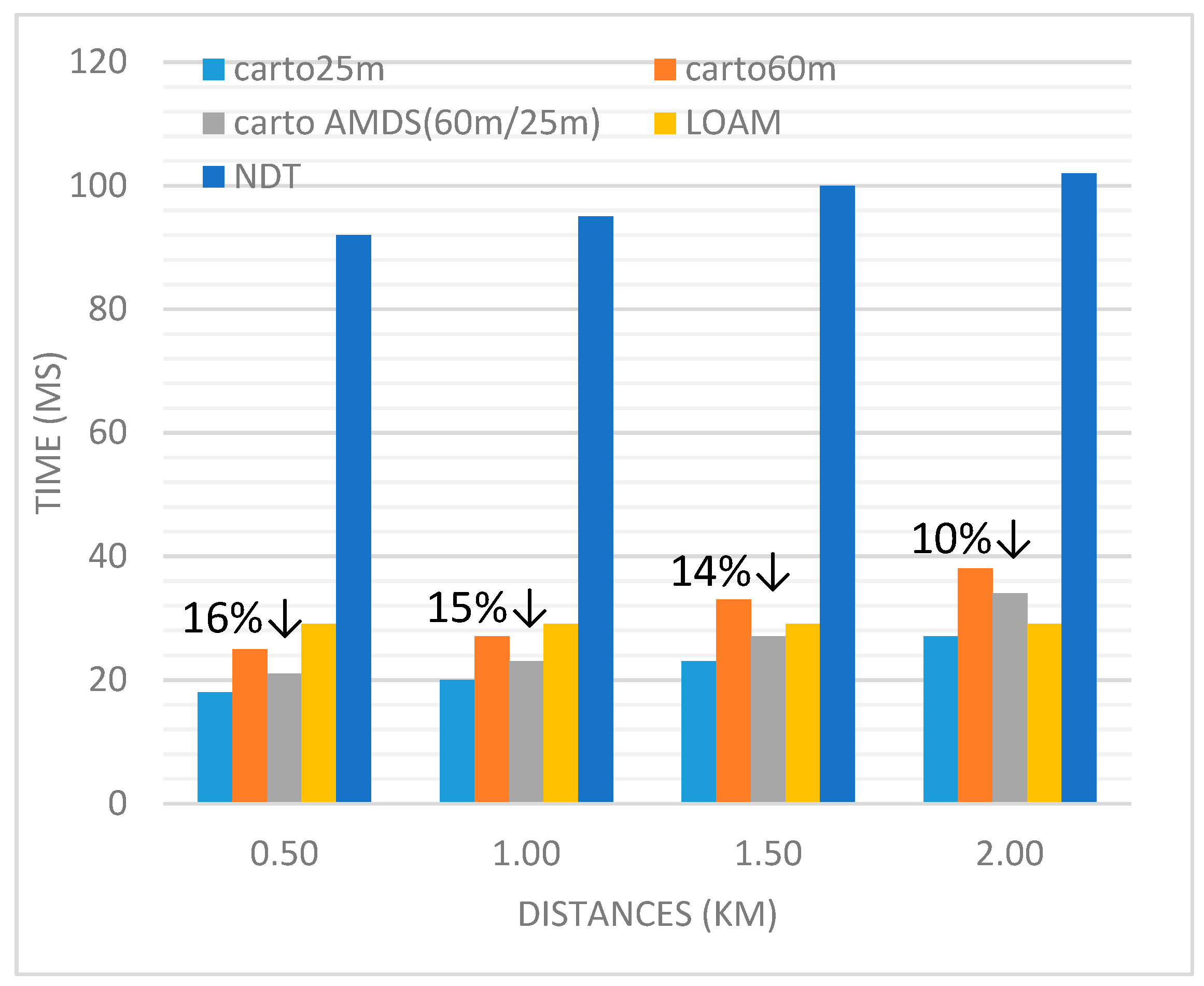
- Optimizing Cartographer by using an adaptive multistage distance scheduler (AMDS) to increase time computation performance up to 20% while maintaining the pose generation and map accuracy similar to that of standard Cartographer;
- (b)
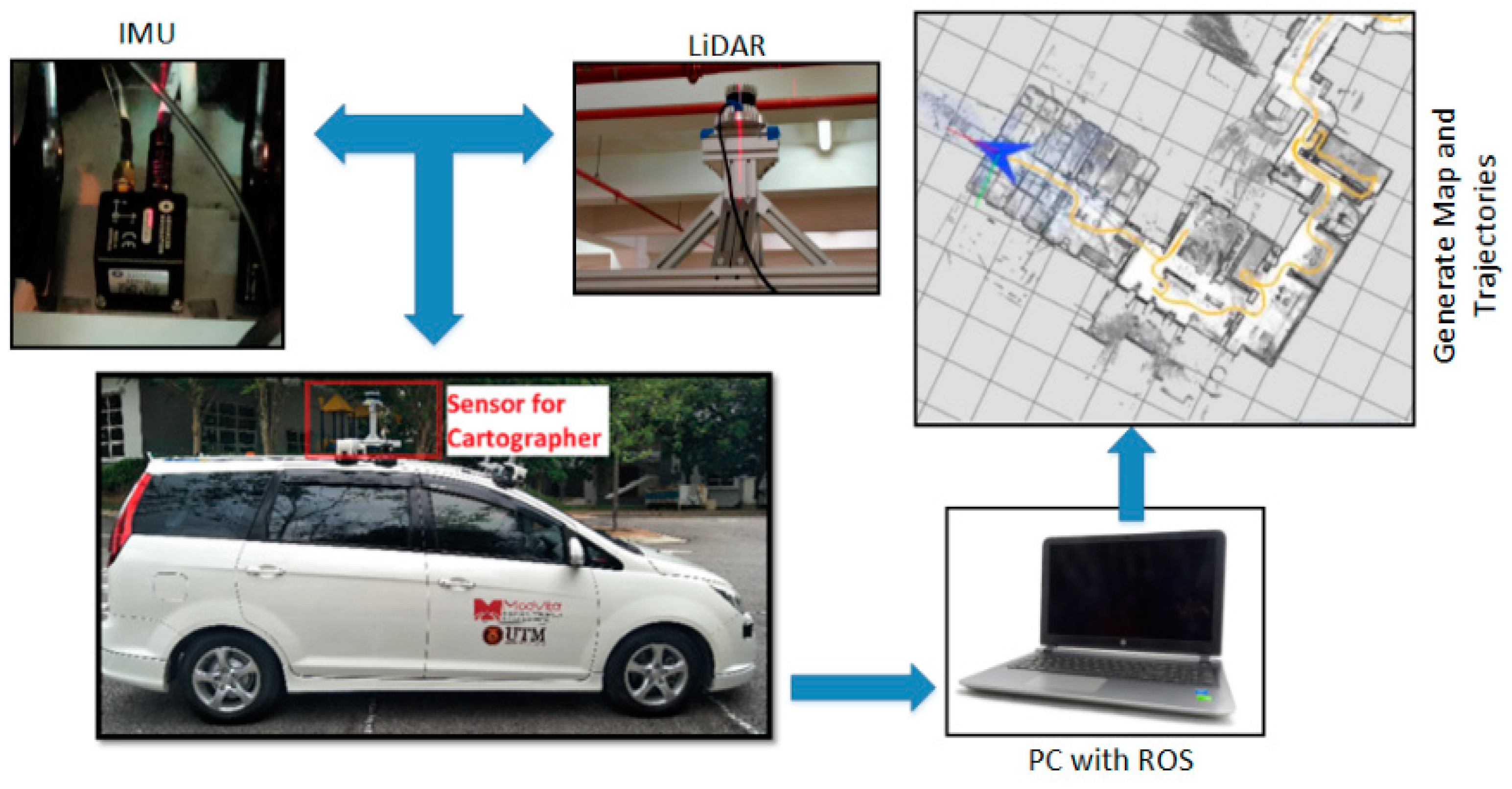
- Integrating Cartographer by using a car for online world mapping, which is crucial for the future autonomous vehicle navigation systems;
- (c)
- Investigating the performance of the proposed method by comparing it to the popular SLAM methods (LiDAR odometry and mapping (LOAM) and normal distribution transform (NDT) SLAM), in the actual world environment.
2. Related Works
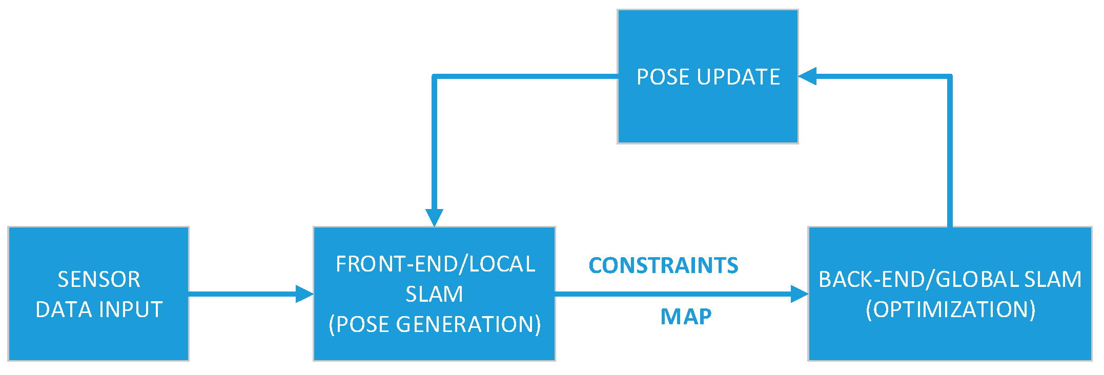
3. System Overview
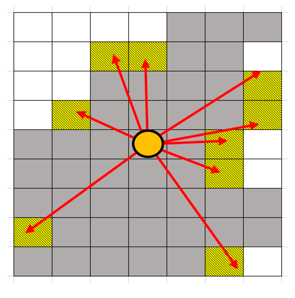
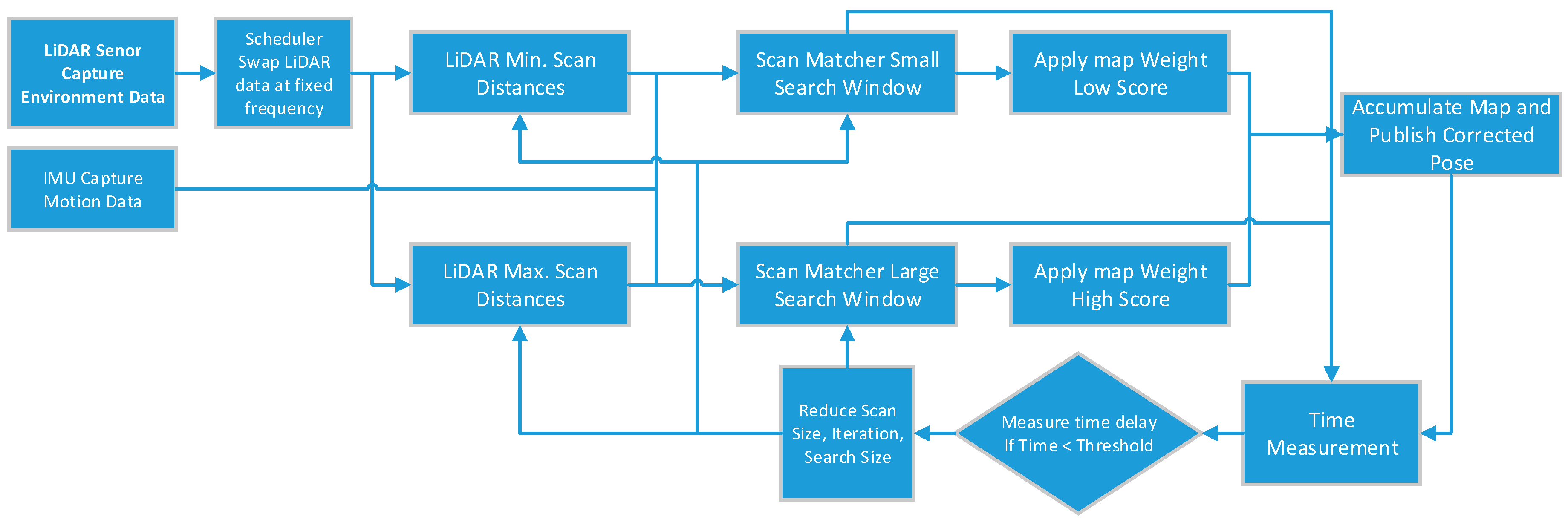
3.1. Multi-Distance Scheduler in LiDAR Scans
3.2. Local SLAM and Map Construction
3.3. Ceres Scan Matching
3.4. Adaptive Performance Control
3.5. Global SLAM Loop Closure
3.5.1. Optimization Problem
3.5.2. Branch and Bound Scan Matching (BBS)
4. Experimental Results
4.1. KITTI Benchmark
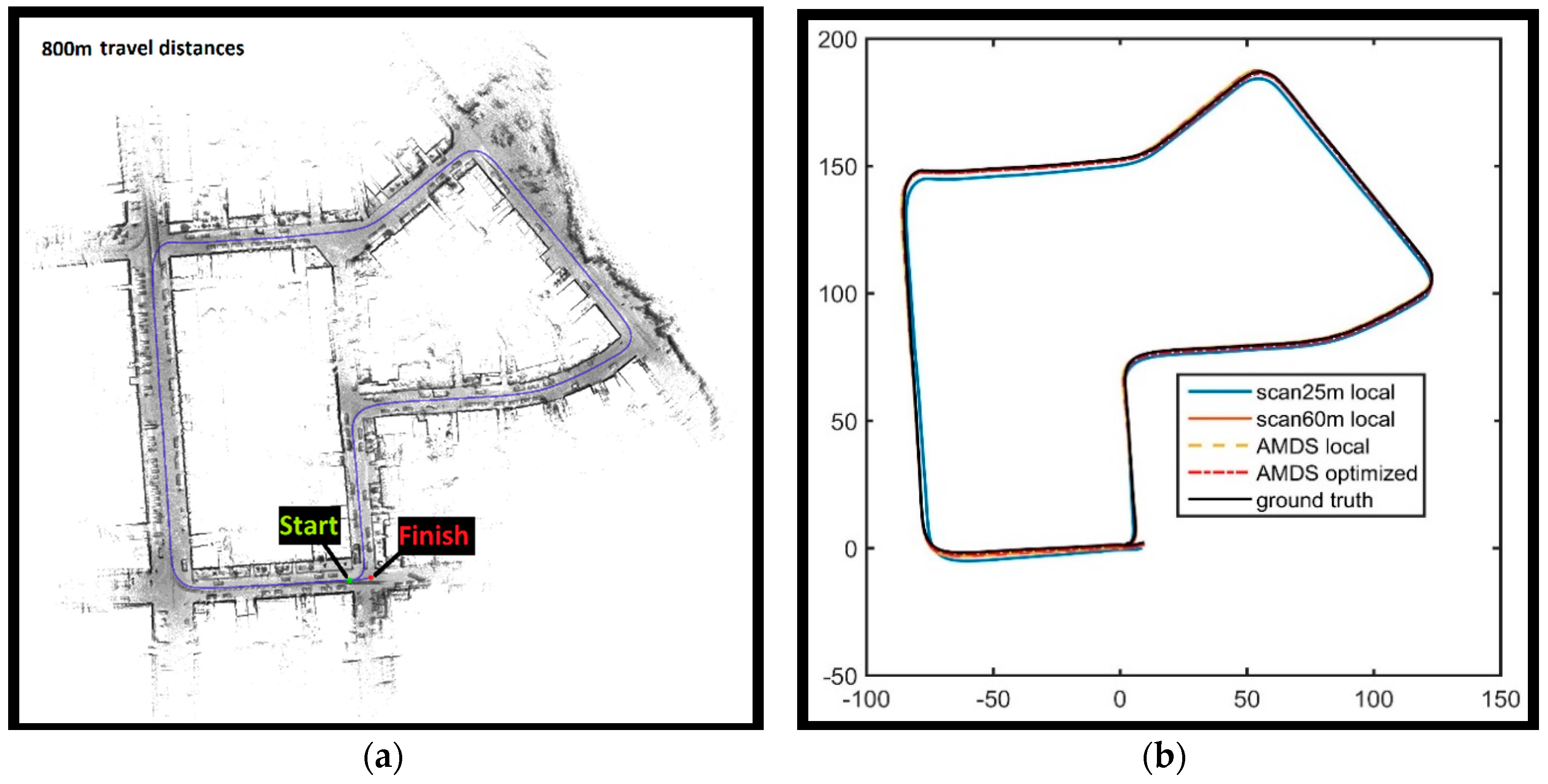
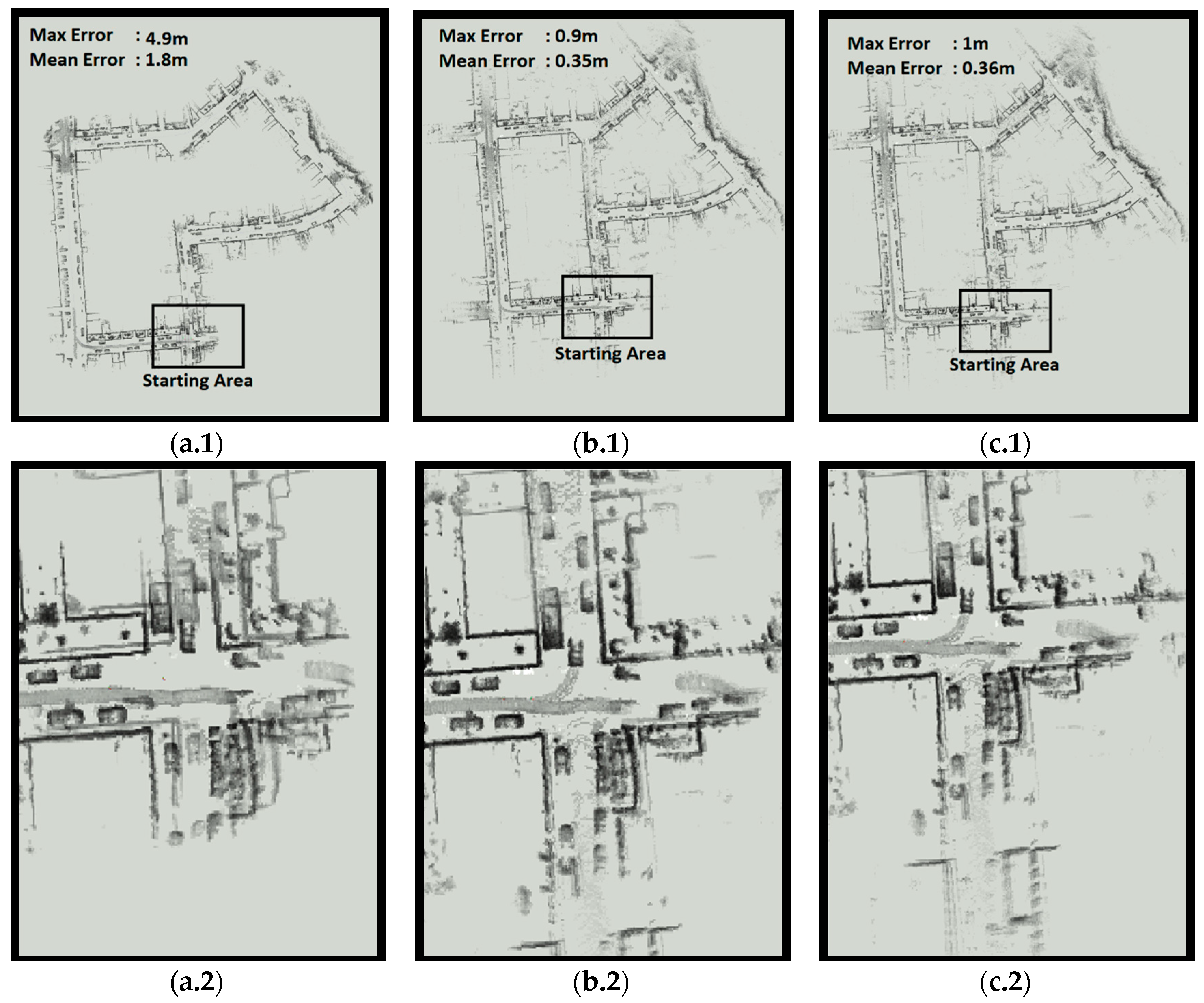
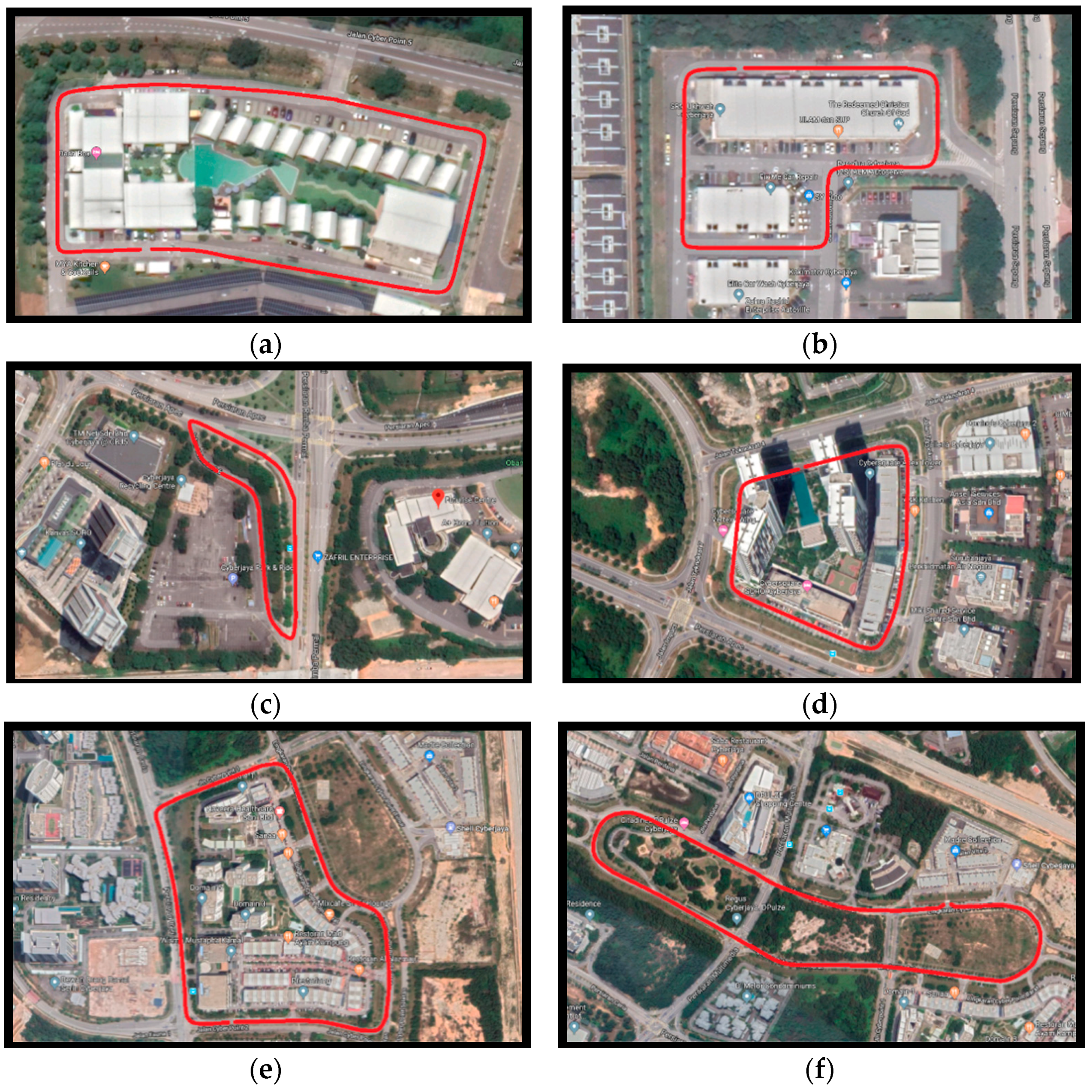
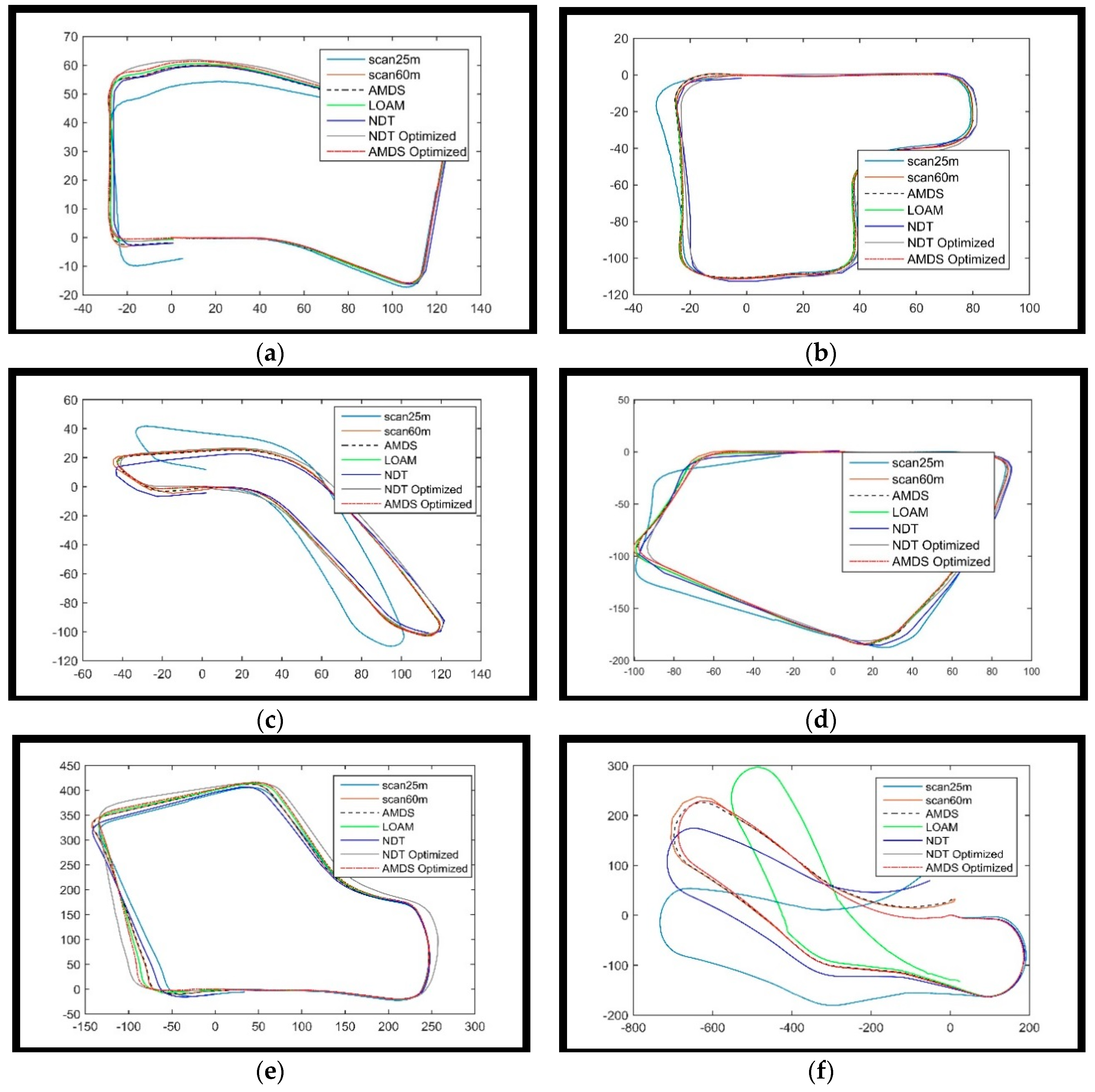
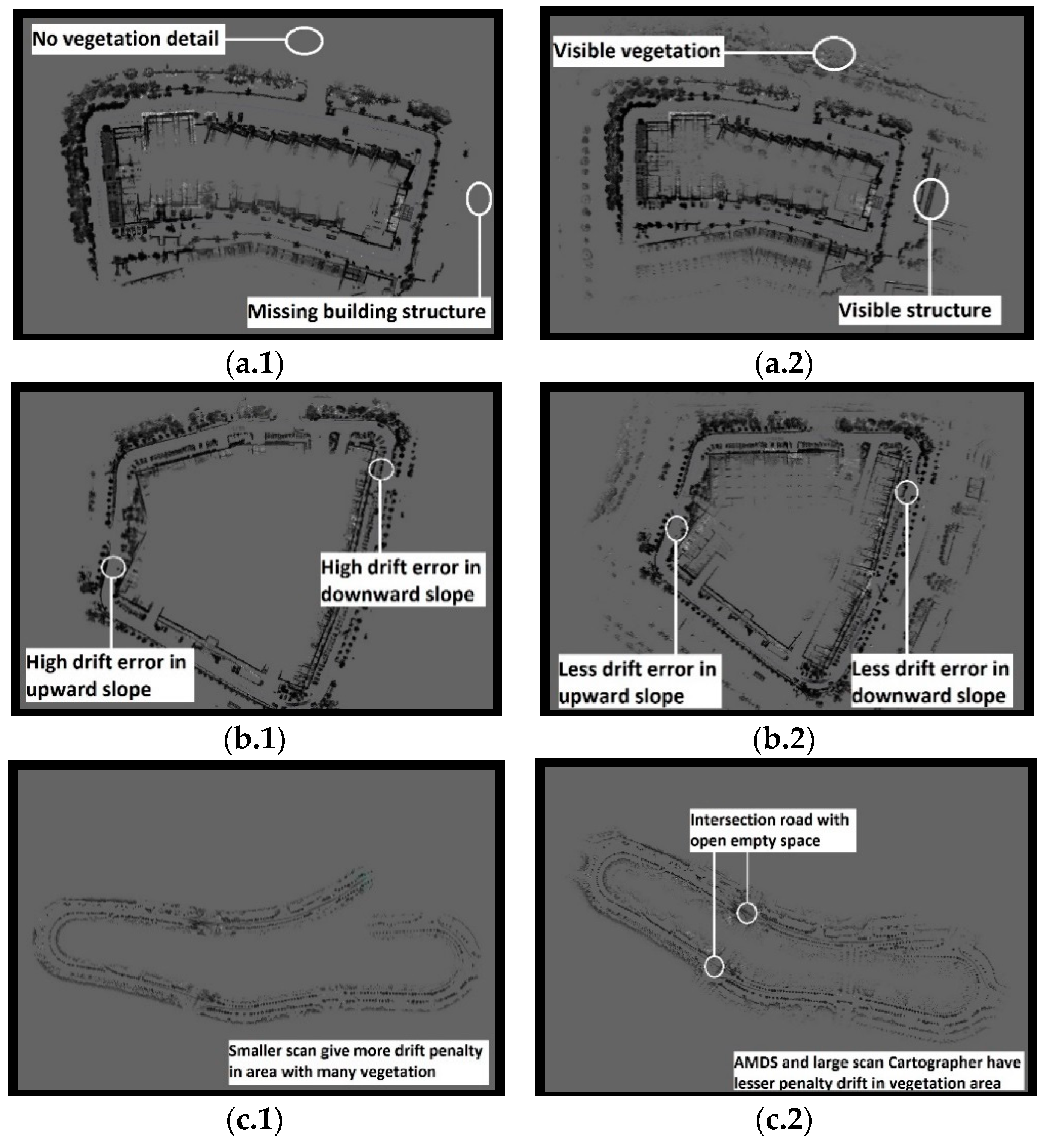
4.2. Experimental Validation
5. Conclusions
Author Contributions
Funding
Acknowledgments
Conflicts of Interest
References
- Hess, W.; Kohler, D.; Rapp, H.; Andor, D. Real-Time Loop Closure in 2D LIDAR SLAM. In Proceedings of the IEEE International Conference on Robotics and Automation (ICRA), Stockholm, Sweden, 16–20 May 2016. [Google Scholar]
- Khairuddin, A.R.; Talib, M.S.; Haron, H. Review on simultaneous localization and mapping (SLAM). In Proceedings of the IEEE International Conference on Control System, Computing and Engineering (ICCSCE), George Town, Malaysia, 25–27 November 2016. [Google Scholar]
- Krinkin, K.; Filatov, A.; Filatov, A.y.; Huletski, A.; Kartashov, D. Evaluation of Modern Laser Based Indoor SLAM Algorithms. In Proceedings of the Conference of Open Innovations Association (FRUCT), Jyvaskyla, Finland, 13–16 November 2018. [Google Scholar]
- Tiar, R.; Lakrouf, M.; Azouaoui, O. FAST ICP-SLAM for a bi-steerable mobile robot in large environments. In Proceedings of the IEEE International Workshop of Electronics, Control, Measurement, Liberec, Czech Republic, 12–13 October 2015. [Google Scholar]
- Bahreinian, S.F.; Palhang, M.; Taban, M.R. Investigation of RMF-SLAM and AMF-SLAM in closed loop and open loop paths. In Proceedings of the International Conference of Signal Processing and Intelligent Systems (ICSPIS), Tehran, Iran, 14–15 December 2016. [Google Scholar]
- Jo, H.; Cho, H.M.; Jo, S.; Kim, E. Efficient Grid-Based Rao–Blackwellized Particle Filter SLAM With Interparticle Map Sharing. IEEE/ASME Trans Mechatron. 2018, 23, 714–724. [Google Scholar] [CrossRef]
- Lee, D.; Kim, H.; Myung, H. GPU-based real-time RGB-D 3D SLAM. In Proceedings of the International Conference on Ubiquitous Robots and Ambient Intelligence (URAI), Daejeon, Korea, 26–28 November 2012. [Google Scholar]
- Ratter, A.; Sammut, C.; McGill, M. GPU accelerated graph SLAM and occupancy voxel based ICP for encoder-free mobile robots. In Proceedings of the IEEE/RSJ International Conference on Intelligent Robots and Systems, Tokyo, Japan, 3–7 November 2013. [Google Scholar]
- Zhang, H.; Martin, F. CUDA accelerated robot localization and mapping. In Proceedings of the IEEE Conference on Technologies for Practical Robot Applications (TePRA), Woburn, MA, USA, 22–23 April 2013. [Google Scholar]
- Song, J.; Wang, J.; Zhao, L.; Huang, S.; Dissanayake, G. MIS-SLAM: Real-Time Large-Scale Dense Deformable SLAM System in Minimal Invasive Surgery Based on Heterogeneous Computing. IEEE Robot. Autom. Lett. 2018, 3, 4068–4075. [Google Scholar] [CrossRef]
- Dine, A.; Elouardi, A.; Vincke, B.; Bouaziz, S. Speeding up graph-based SLAM algorithm: A GPU-based heterogeneous architecture study. In Proceedings of the IEEE 26th International Conference on Application-specific Systems, Architectures and Processors (ASAP), Toronto, ON, Canada, 27–29 July 2015. [Google Scholar]
- Kohlbrecher, S.; Stryk, O.V.; Meyer, J.; Klingauf, U. A flexible and scalable SLAM system with full 3D motion estimation. In Proceedings of the IEEE International Symposium on Safety, Security, and Rescue Robotics, Kyoto, Japan, 1–5 November 2011. [Google Scholar]
- Jang, J.; Kim, J. Dynamic Grid Adaptation for Panel-Based Bathymetric SLAM. In Proceedings of the IEEE Underwater Technology (UT), Kaohsiung, Taiwan, 16–19 April 2019. [Google Scholar]
- Oršulić, J.; Miklić, D.; Kovačić, Z. Efficient Dense Frontier Detection for 2-D Graph SLAM Based on Occupancy Grid Submaps. IEEE Robot. Autom. Lett. 2019, 4, 3569–3576. [Google Scholar] [CrossRef]
- Ristic, B.; Angley, D.; Selvaratnam, D.; Moran, B.; Palmer, J.L. A random finite set approach to occupancy-grid SLAM. In Proceedings of the 19th International Conference on Information Fusion (FUSION), Heidelberg, Germany, 5–8 July 2016. [Google Scholar]
- Biber, P.; Strasser, W. The normal distributions transform: A new approach to laser scan matching. In Proceedings of the International Conference on Intelligent Robots and Systems, Las Vegas, NV, USA, 27–31 October 2003. [Google Scholar]
- Rapp, M.; Barjenbruch, M.; Hahn, M.; Dickmann, J.; Dietmayer, K. Clustering improved grid map registration using the normal distribution transform. In Proceedings of the Intelligent Vehicles Symposium (IV), Seoul, Korea, 29 June–1 July 2015. [Google Scholar]
- Zhang, J.; Singh, S. LOAM: Lidar Odometry and Mapping in Real-time. In Proceedings of the Robotics: Science and Systems Conference, Pittsburgh, PA, USA, 12–16 July 2014. [Google Scholar]
- Mur-Artal, R.; Tardós, J.D. ORB-SLAM2: An Open-Source SLAM System for Monocular, Stereo, and RGB-D Cameras. IEEE Trans. Robot. 2017, 33, 1255–1262. [Google Scholar] [CrossRef]
- Cheng, Z.; Wang, G. Real-Time RGB-D SLAM with Points and Lines. In Proceedings of the 2nd IEEE Advanced Information Management, Communicates, Electronic and Automation Control Conference (IMCEC), Xi’an, China, 25–27 May 2018. [Google Scholar]
- Wu, D.; Meng, Y.; Zhan, K.; Ma, F. A LIDAR SLAM Based on Point-Line Features for Underground Mining Vehicle. In Proceedings of the Chinese Automation Congress (CAC), Xi’an, China, 30 November–2 December 2018. [Google Scholar]
- Greene, W.N.; Ok, K.; Lommel, P.; Roy, N. Multi-level mapping: Real-time dense monocular SLAM. In Proceedings of the Multi-level mapping: Real-time dense monocular SLAM, Stockholm, Sweden, 16–20 May 2016. [Google Scholar]
- Olson, E. M3RSM: Many-to-many multi-resolution scan matching. In Proceedings of the International Conference on Robotics and Automation (ICRA), Seattle, WA, USA, 26–30 May 2015. [Google Scholar]
- Agarwal, S.; Mierle, K. Ceres Solver. Available online: http://ceres-solver.org (accessed on 2 July 2019).
- Shen, Q.; Sun, H.; Ye, P. Research of large-scale offline map management in visual SLAM. In Proceedings of the International Conference on Systems and Informatics (ICSAI), Hangzhou, China, 11–13 November 2017. [Google Scholar]
- Konolige, K.; Grisetti, G.; Kümmerle, R.; Burgard, W.; Limketkai, B.; Vincent, R. Sparse Pose Adjustment for 2D Mapping. In Proceedings of the IROS, Taipei, Taiwan, 18–22 October 2010. [Google Scholar]
- Geiger, A.; Lenz, P.; Urtasun, R. Are we ready for Autonomous Driving? The KITTI Vision Benchmark Suite. In Proceedings of the Conference on Computer Vision and Pattern Recognition (CVPR), Washington, DC, USA, 16–21 June 2012. [Google Scholar]
- Quigley, M.; Gerkey, B.P.; Conley, K.; Faust, J.; Foote, T.; Wheeler, R.; Leibs, J.; Ng, A.Y. ROS: An open-source Robot Operating System. In Proceedings of the ICRA Workshop on Open Source Software, 17 May 2009. [Google Scholar]
- Hong, S.; Ko, H.; Kim, J. VICP: Velocity updating iterative closest point algorithm. In Proceedings of the IEEE International Conference on Robotics and Automation, Anchorage, AK, USA, 3–8 May 2010. [Google Scholar]
- Kümmerle, R.; Steder, B.; Dornhege, C.; Ruhnke, M.; Grisetti, G.; Stachniss, C.; Kleiner, A. On measuring the accuracy of SLAM algorithms. Auton. Robot 2009, 27, 387–407. [Google Scholar] [CrossRef]


| Function Multi-distance scheduler (PointsCloud_, Period_ratio_on, Max_Distances, Min_Distances) if (step scheduler == Period_ratio_time_on) for all p_point in PointsCloud_ do if (p_point > Max_Distances) Null p_point(x,y,z) in PointClouds data end if end for end if if (step scheduler != Period_ratio_time_on) for all p_point in PointsCloud_ do if (p_point > Min_Distances) Null p_point(x,y,z) in PointsCloud_ data end if end for end if Step scheduler = Step scheduler + current_time return PointsCloud_ end function |
| best_score ← Null for jx = - to do for jy = - to do for jθ = - to do score ← if score > best_score then match ← best-score ← score end if end for end for end for return best-score and match |
| score_thresold -> best_score Compute and memorize a score for each element in C0. Initialize a stack C with C0 sorted by score, the maximum score at the top. while C is not empty do Pop c from the stack C if score(c) > best_score then perform leaf selection (·) end if end if | Leaf selection (·) if C is leaf node then c-> match. score(c) -> best_score. else Branch: split c into nodes Cc. Compute and memorize a score for each element in Cc. Push Cc onto the stack C, sorted by score, the maximum score last. end if return |
| Map 1 | Map 2 | Map 3 | Map 4 | Map 5 | Map 6 | |||||||
|---|---|---|---|---|---|---|---|---|---|---|---|---|
| m | ° | m | ° | m | ° | m | ° | m | ° | m | ° | |
| Carto25 m local/unoptimized | 8.9 | 10.3 | 9.7 | 9.5 | 11.1 | 9.9 | 9.7 | 17.5 | 34.3 | 7.7 | 110 | 35.9 |
| Carto60 m local/unoptimized | 2.0 | 1.4 | 0.4 | 1.3 | 7.6 | 2.6 | 0.5 | 15 | 13.9 | 5.1 | 35 | 9.5 |
| AMDS (60 m/25 m) Local/unoptimized | 2.1 | 1.4 | 0.4 | 1.3 | 7.6 | 2.6 | 0.6 | 1.5 | 15.9 | 5.0 | 37 | 9.6 |
| LOAM Unoptimized | 10 | 0.5 | 1.1 | 0.5 | 2.6 | 1.4 | 1.0 | 0.5 | 5.8 | 5.0 | 135 | 19.9 |
| NDT unoptimized | 1.9 | 1.3 | 2.5 | 2.9 | 4.6 | 2.1 | 3.7 | 1 | 9.6 | 3.7 | 81 | 37 |
| NDT optimized | 0.3 | 0.5 | 0.3 | 0.5 | 0.2 | 0.7 | 0.4 | 0.7 | 0.4 | 2.0 | 0.1 | 1.9 |
| AMDS (60 m/25 m) Optimized | 0.2 | 0.5 | 0.2 | 0.5 | 0.3 | 0.7 | 0.2 | 0.8 | 0.5 | 1.7 | 0.2 | 1.9 |
© 2020 by the authors. Licensee MDPI, Basel, Switzerland. This article is an open access article distributed under the terms and conditions of the Creative Commons Attribution (CC BY) license (http://creativecommons.org/licenses/by/4.0/).
Share and Cite
Dwijotomo, A.; Abdul Rahman, M.A.; Mohammed Ariff, M.H.; Zamzuri, H.; Wan Azree, W.M.H. Cartographer SLAM Method for Optimization with an Adaptive Multi-Distance Scan Scheduler. Appl. Sci. 2020, 10, 347. https://doi.org/10.3390/app10010347
Dwijotomo A, Abdul Rahman MA, Mohammed Ariff MH, Zamzuri H, Wan Azree WMH. Cartographer SLAM Method for Optimization with an Adaptive Multi-Distance Scan Scheduler. Applied Sciences. 2020; 10(1):347. https://doi.org/10.3390/app10010347
Chicago/Turabian StyleDwijotomo, Abdurahman, Mohd Azizi Abdul Rahman, Mohd Hatta Mohammed Ariff, Hairi Zamzuri, and Wan Muhd Hafeez Wan Azree. 2020. "Cartographer SLAM Method for Optimization with an Adaptive Multi-Distance Scan Scheduler" Applied Sciences 10, no. 1: 347. https://doi.org/10.3390/app10010347
APA StyleDwijotomo, A., Abdul Rahman, M. A., Mohammed Ariff, M. H., Zamzuri, H., & Wan Azree, W. M. H. (2020). Cartographer SLAM Method for Optimization with an Adaptive Multi-Distance Scan Scheduler. Applied Sciences, 10(1), 347. https://doi.org/10.3390/app10010347