Abstract
Ultra-wideband (UWB) is considered as a promising technology in short-distance indoor wireless positioning due to its accurate time resolution and good penetration through objects. Since the functional model of UWB positioning is nonlinear, the optimal solution is generally estimated by the way of continuous iteration. As an iterative descent method of high efficiency, the Gauss–Newton method is widely used to estimate the position. The nonlinear distance equations are linearized, and the solution can be found iteratively. Therefore, the nonlinear least-squares solution is generally biased even if the observations are normally distributed. In outdoor satellite positioning, the ranging distances are long enough so that the bias caused by nonlinearity is very small. However, in UWB positioning, the relative ranging error is large, and the positioning system is prone to become ill-posed, hence the bias due to nonlinearity is not negligible. In this study, both the statistical factor and geometric factor for bias in the nonlinear least-squares estimator of UWB positioning are discussed. In order to assess whether the linearized model is sufficiently approximate for the positioning estimation, a hypothesis test criterion based on Mahalanobis distance is proposed. The simulation and measurement experiments are performed to analyze the factors affecting the bias in UWB positioning. Experimental results are given to demonstrate that the linearization is valid and the bias in UWB positioning estimation can be neglected for the relatively high measurement precision. Moreover, for a positioning configuration, when the anchors are evenly distributed, the amount of nonlinearity is orthogonal to the ranging space of the design matrix, the UWB positioning estimation tends to be unbiased. Meanwhile, the hypothesis test based on Mahalanobis distance is carried out to determine the validity of the linearized model. When the bias is large for UWB positioning, the bias estimate can be used to correct the estimator to guarantee the unbiasedness for UWB positioning. Furthermore, the correction of parameter estimator bias is more effective in the case of relatively low measurement precision or ill-conditioned configuration.
1. Introduction
High accuracy position information is of great importance in many surveying and navigation applications. During recent decades, with the development of global navigation satellite system (GNSS), people pay more and more attention to the location based on service [1]. Urban dwellers spend more than 80% of their time indoors. However, the intensity of GNSS signal is not strong enough to penetrate through different materials used in construction, and the phenomena of reflection and multipath fading limit the utility of GNSS in dense urban or in the indoor environment, which increases the demand for indoor positioning [2,3]. In general, indoor positioning technologies include: Bluetooth, Wi-Fi, radio-frequency identification (RFID), ultra-wideband (UWB) and so on [4]. Compared with other localization technologies, the UWB is capable of providing robust signaling, through-wall propagation [5]. Due to a large bandwidth, it can obtain high-resolution distance estimation and enables reliable distance estimation. Therefore, UWB technology is well-suited for indoor positioning applications.
In order to employ this technology, different positioning methods have been developed. The positioning system can employ various information obtained from radio signals, such as time-of-arrival (TOA), time difference of arrival (TDOA), angle of arrival (AOA), and received signal strength (RSS) [6]. The accuracy of positioning system in term of positioning, ranging and navigation could reach easily a decimeter level. However, in order to provide the position, it depends on the network installation and this could represent a limitation in term of cost, time and infrastructure requirements [7]. The performance of a dynamic ad-hoc UWB-based positioning system was introduced, which can accommodate any arbitrary number of nodes operating in the same region, additionally. it can provide much more flexibility to supports the dynamic inclusion or removal of nodes from the network [8]. To solve the limitation in terms of tag density, a UWB indoor localization system that allows an unlimited number of tags was presented, it allows tags to obtain responses from multiple anchors simultaneously. This system enables decimeter-level accuracy at fast update rates for countless tags and is highly suited for supporting mobile applications [9]. Meanwhile, to ensure people and objects can be localized in real-time, the integration of UWB and other technologies such as RFID and Wi-Fi are developed. The passive UWB RFID based on the backscatter modulation signal increases significantly the performance for tags detection and localization at low and complexity by employing energy sprinklers [10,11,12]. The integration of UWB and Wi-Fi are implemented for localization, the Wi-Fi networks guarantee broad coverage while the UWB would increase the overall system accuracy and robustness [13].
In practical applications, an unbiased estimation of the positioning result will be expected. However, the positioning estimation is subject to different error sources, including signal blockage, multipath, clock drift, algorithm model, thermal noise and so on. Meanwhile, the positioning system is prone to become ill-posed. The performance and the reliability of the positioning algorithms are inevitably influenced. Although the use of UWB signals can resolve these multipath components, however, the large number of multipath components in harsh environments makes direct path (DP) detection nontrivial. In addition, both the relative clock offsets as well as response delay strongly affect ranging accuracy [14]. UWB ranging with the appropriate error calibration methods is able to provide indoor positioning of high accuracy in the centimeter level, but it requires to perform the calibration for each indoor area of interest in advance [15]. A nonparametric machine learning approach is employed to estimate the ranging error directly from the received waveform without any a priori or a posteriori knowledge, and it has the potential to significantly improve localization performance [16]. Ranging based on the RSS is very sensitive to the path loss model, and a better placement of the base stations could bring better accuracy through better geometrical condition [17]. Moreover, an accurate indoor positioning system requires more than just accurate range measurements. Its performance is affected by the number and the configuration of the anchor, along with the accuracy of the anchor positions.
In general, the error in the functional model will have more serious consequences for the parameter estimation than that of the stochastic model. The functional model of UWB positioning is nonlinear. The best method is Taylor’s expansion of the nonlinear distance equations, and then the approximate solutions can be obtained iteratively [18,19]. As a standard method for solving general nonlinear equations, the Gauss–Newton iteration is efficient and has a linear convergence rate for points close to the solution [20]. However, the estimation is usually inherently biased by linearizing the nonlinear expression, and the bias is derived from non-zero higher-order terms [21]. The bias in nonlinear least-squares estimator is studied to show that the relatively high precision of geodetic measurements often makes bias negligible, despite strong non-linearity in the functional model [22,23]. The amount of nonlinearity of the model is related to the curvature of the manifold and the parameter curves with a differential geometry point of view [24]. As a differential geometric interpretation, the bias in parameter vector depends on the parametrization which is known as geodetic coordinates, and the bias in residual vector is determined by the mean curvature of manifold [25]. For short-distance indoor positioning, the bias in the nonlinear least-squares solution should be detected and the estimation can obtain unbiased values by removing the bias from the nonlinear least-squares solution [26,27]. Therefore, we deem it essential to discuss the factors contributing to the bias and how the Taylor remainder affects the parameter estimators in nonlinear least-squares problems.
Statistical testing for modelling errors and biases is an important component in data quality control [28]. The DIA (detection, identification and adaptation) method of model misspecifications combines parameter estimation with a hypothesis test with the aim to remove any biases that may be present [29,30]. The minimal detectable bias (MDB) of an alternative hypothesis is the smallest outlier that can lead to rejection of a null hypothesis. The MDB describes the internal reliability, and the value propagated into the parameters is said to describe the external reliability [31]. Under the assumption with Gaussian distribution, the Chi-square test is performed to identify and exclude the suspected observations corresponding to these faults [32,33]. A judging index is defined as the square of the Mahalanobis distance from the observation to its prediction, and the hypothesis test is performed to the actual observation by treating the judging index as the test statistic [34].
In particular, the remainder of this paper is organized as follows: In Section 2, the nonlinear least-squares solution of overdetermined distance equations is introduced. In Section 3, the bias estimation based on the linearization adjustment is derived and discussed. In Section 4, a judging index for the hypothesis test based on Mahalanobis distance is proposed. In Section 5, the influences on the bias in nonlinear least-squares estimators are illustrated and analyzed by the numerical examples. In Section 6, the conclusions are summarized.
2. The Nonlinear Least-Squares Solution of Distance Equations in UWB Positioning
As is shown in Figure 1, we evaluate UWB sensor network positioning system based on the DW1000 module. After collecting ranging data by the positioning system, the position of the tag can be determined by solving the nonlinear distance equations. The system dealing with UWB positioning in this paper is based on TOA, the ranging measurements in these transceivers is performed based on the two-way ranging (TWR) in which the positioning system estimates the signal round-trip time (RTT) without a common time reference and eliminates the error due to imperfect synchronization [35,36].
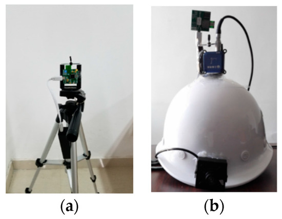
Figure 1.
The anchor (a) and tag (b) hardware devices.
The nonlinear observation model of distance equation is given as [37]:
where denotes the observation vector; is the coordinate vector of tag; represents the corresponding ranging random error; is the Euclidean distance, is the known coordinate of th anchor. is the coordinate of tag.
If the nonlinear equations are over-determined, then the nonlinear least-squares solution is to find , where , in which represents the residual vector, and the least squares solution of coordinate correction can be written as:
where is the Jacobian matrix of distance equations, is the direction cosine vector from the tag to the anchor.
With a rough initial value
and Equation (2), we can obtain the least squares solution by way of the Gauss–Newton method with iterations:
Considering this positioning system eliminates the clock offset, the coefficient matrix of coordinate vector of unknown point can be obtained as:
The position dilution of precision (PDOP), horizontal dilution of precision (HDOP) and vertical dilution of precision (VDOP) are defined as:
Dilution of precision (DOP) describes the relationship between measure error and position determination, and it is similar to the satellite positioning. The more observations used, the smaller the DOP values and hence the smaller the solution error.
3. The Bias in the Nonlinear Least-Squares Solution
The nonlinear least-squares estimator can be written as a function of the random observation vector :
Generally speaking, there is no closed expressions available for the nonlinear observation model, therefore the nonlinear least-squares solution cannot be given explicitly. A Taylor expansion for the estimator is given as:
If the terms of the third order and higher are ignored, take the expectation of the Equation (7), then the bias in the nonlinear least-squares parameter estimator can be expressed as [22]:
where , represents the variance matrix of the observation vector. We can see that the bias comes from non-zero higher order terms. Assuming that the observations are normally distributed, the least-squares estimator is equivalent to the maximum likelihood estimator, then , and will be an unbiased estimator of , and Equation (8) can be simplified to:
For the nonlinear cases, is non-zero, and therefore, the least-squares estimator is biased. Based on the orthogonality condition, we can get the first and second order partial derivatives of the function , then the bias is finally estimated [24]:
where is the amount of nonlinearity.
According to Taylor’s theory, the distance function is obtained as follows [21]:
We can see that is actually the expected difference between the linear and quadratic approximation of the distance function , and it can be expressed as [27]:
Equation (10) shows that the bias is in nonlinear least-squares estimator of the distance equations is driven by the covariance matrix and the second order derivatives matrix . It means that the bias due to nonlinearity is related to both the system geometry and the precision of the estimator. Equation (12) indicates that the bias in the nonlinear least-squares estimator is inversely proportional to the ranging distance and is proportional to the ranging error. The bias will be small if is sufficiently close to zero, so that the model is essentially linear, or if is orthogonal to the column space of design matrix . Equations (10) and (12) make us know the factors contributing to the bias.
4. The Hypothesis Test Based on Mahalanobis Distance for the Bias Check
The parameter estimator bias can be a potential problem for UWB positioning. To check if the bias in nonlinear least-squares estimator is too large, the hypothesis test based on Mahalanobis distance is proposed.
where denotes the Mahalanobis distance, is the square of Mahalanobis distance and is the test statistic term, is the parameter estimator with Gaussian distribution considering only the first-order Taylor expansion, is the parameter solution ignoring the terms of the third order and higher. The test statistic term is the Mahalanobis distance, which can be a measure of significance [38].
The hypothesis test can be carried out for testing the bias:
where is predetermined 3.84 by the chosen level of significance being 0.05 based on Chi-square distribution table.
By assuming that the observations obey Gaussian distribution, when the parameter estimator bias is small, the Mahalanobis distance is smaller than the threshold of the test statistic, and should be Chi-square distributed with the dimension of the observation vector as the degree of freedom (DOF). If is larger than , and the value of test statistic will fall in the right tail-area of the distribution and the null hypothesis can be rejected. We can believe that the model error for UWB positioning does occur, and the linearized model is not sufficiently approximate. The results show that since the large bias due to nonlinearity in UWB position, the estimator needs to be corrected to endure the unbiasedness for UWB positioning.
5. Numerical Examples
In this section, we will analyze the parameter estimator bias by simulation and measurement experiments. For each test, the bias is estimated by Gauss-Newton method. Being close enough to the least-squares solution is one of the sufficient conditions for convergence to occur. The well-conditioned initial values for the iteration are set to ensure the correct convergence. We should note that if the measurement error is small, it can happen that the final estimator is closer to the true position. For each fixed configuration with one specific standard deviation, the parameter estimator bias is obtained by the Equation (10). To check if the bias is significant, the hypothesis test is performed to compare the Mahalanobis distance and the threshold which is 1.96.
5.1. Simulation Verification
In the simulation experiment, the bias estimation is based on the Monte Carlo method, five positioning system configurations are tested, which differ in the anchor-tag positions and redundancy. The coordinates of the anchor and tag are shown in Figure 2. The distance between the tag and the anchor in Configurations 1, 2 and 3 are all the same, which is calculated to be cm. The simulated measurement error obeys the normal distribution which is an independent Gaussian variable with zero mean and equal variance. The standard deviation of the first four sets and the sixth set is 5 cm. Both the fourth and fifth set of tests are based on Configuration 4. The fifth set of test is carried out by simulating large noise with the standard deviation of 18 cm, representing the variety of the observation variance. The observation model equation is simulated 10,000 times for detecting the bias in nonlinear least-squares estimator.
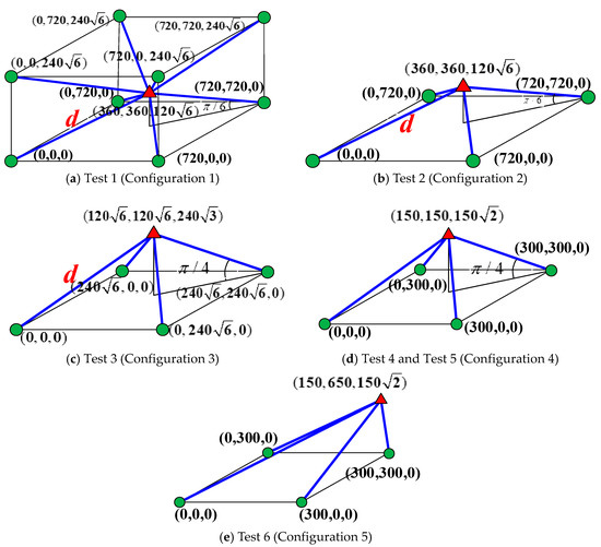
Figure 2.
The tests and positioning configurations.
The frequency histograms of parameter estimator bias are given in Figure 3. The average PDOP, HDOP and VDOP are shown in Figure 4.
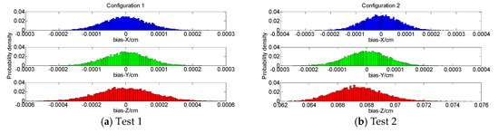
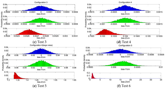
Figure 3.
The frequency histograms of parameter estimator bias.
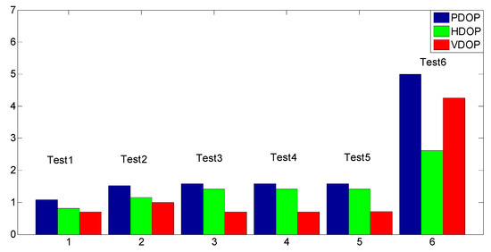
Figure 4.
The average position dilution of precision (PDOP), horizontal dilution of precision (HDOP) and vertical dilution of precision (VDOP) for each set of tests.
In Test 1 based on Configuration 1, there are adequate redundant observations, and the anchors are uniformly distributed in the three-dimensional (3D) space. The three types of DOP values in this group are the smallest. The average bias of coordinate components x, y and z are close to zero. This indicates that the least-squares estimator is approximately unbiased, with the reason that the amount of nonlinearity is orthogonal to the column space of the design matrix in this configuration. It makes us know that Configuration 1 is suitable for the traditional indoor positioning, and it also can achieve satisfactory accuracy.
In the next five sets of tests, there is only one redundant observation with anchors distributed on a planar ground. This makes the number of parameters to be estimated relatively more for the particular observation model, and the nonlinear strength increases with the decreases of DOF. As similar to Test 1, the coordinate components x and y are also unbiased in Tests 2, 3, 4 and 5, but the coordinate component z is biased. It indicates that the corresponding component does not satisfy the orthogonal condition with the zero bias because of the ill-conditioned positioning configuration. Moreover, when the distance between the tag and the anchor and the ranging measurement noise are fixed in the Test 2 and 3 based on Configuration 2 and 3, it makes known that their amount of nonlinearity is equal. The average VDOP in Test 3 is smaller than that in the Test 2, and it has smaller bias in the coordinate component z. In this case, it indicates that the better the system geometry, the smaller the bias in the nonlinear least-squares estimator.
In addition, the Tests 3, 4 and 5 have the identical geometry. The difference is that Test 4 based on Configuration 4 is scaled down compared with Configuration 3 and Test 5 has larger ranging measurement noise than that of the Test 4. The bias in Test 4 is greater than that of the Test 3, and the bias in Test 5 is largest among these three sets of tests. The results verify that the bias is inversely proportional to the ranging distance and directly proportional to the ranging error.
In Test 6, the tag has the same z coordinate as Test 5, but it is located outside the square enclosed by the anchors. The coordinate components x is unbiased, but both the coordinate component y and z are biased. The three types of DOP values in this group are larger than those in the previous five sets of tests. As we can see, Test 6 based on Configuration 5 has the worst system geometry.
To check if the parameter estimator bias is too large, the hypothesis test based on Mahalanobis distance is implemented. It is used to assess whether the linearized model is a sufficient approximation. The results of six sets of tests and the threshold are compared in Figure 5. We can see that the test statistic of the first four sets of tests are all very small, the latter two sets of tests are very large, and some epoch data exceeds the threshold. It indicates that the bias of some epoch in Tests 5 and 6 are too large and the linearized model is not sufficiently approximate for UWB positioning. The bias is only intolerable for the relative large ranging error and ill-conditioned system geometry. The positioning system performances be ranked as Configuration 1 > Configuration 3 > Configuration 2 > Configuration 4 > Configuration 4 (large noise) and Configuration 5, from good to poor. Furthermore, the statistics of bias correction are listed in Table 1. It can be known that the bias correction effect in the coordinate component x and y can be ignored, and it is obvious in the coordinate component z. We can believe that it is more effective to use second-order bias correction when the measurement precision is relatively low or the configuration is bad.
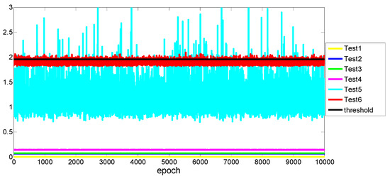
Figure 5.
The hypothesis test based on Mahalanobis distance.

Table 1.
The statistics of bias correction (cm).
5.2. Measurement Verification
In the measurement experiment, the hardware devices used are the DecaWave Mini2016 suite, including the anchor and tag nodes, already described in detail in Section 2. The experimental scene is an empty hall of 10 m by 18 m. During the testing process, no relevant personnel entered. The data sampling interval of the positioning system is about 0.28 s. The tag node is mounted on the top of the helmet, which is placed at test point at the height of 30 cm in a static situation and is worn on the human head at a height of 196 cm in a dynamic situation. The anchor nodes are placed on a tripod of the same antenna height. The static and dynamic tests analyses are as follows.
5.2.1. Static Test
The main goal of this test is to evaluate the bias of least-squares parameter estimator under a static situation. The locations of test points and anchors and the experimental scene are shown in Figure 6. The positions of test points were calibrated ahead of time. In the test, 300 epoch data was sampled at each test point.
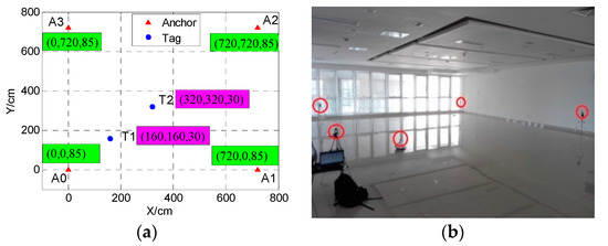
Figure 6.
The locations of test points and anchors (a) and the experimental scene (b).
Figure 7 represents the cumulative distribution function (CDF) of the ranging error of all the measurements collected. It can be observed that the random error of these observations are small and differ slightly. However, all of their systematic errors are very large. The distance between T1 to A1 perfectly matches the distance between T1 and A3, but the range estimation accuracy is different due to the hardware. Although the hardware devices adopt the principle of TWR without a common time reference, the clock drift and offset still affect the ranging error. We can also see that the systematic error based on anchor A1 and A3 becomes larger than that based on anchor A0 and A2.
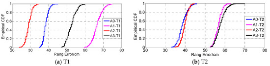
Figure 7.
The cumulative distribution function (CDF) of the ranging error.
The frequency histograms of the parameter estimator bias are given in Figure 8. The average PDOP, HDOP and VDOP for two test points are shown in Figure 9. The anchors are uniformly distributed on a planar ground. The two test points constitute two different positioning configurations with anchors. The three kinds of DOP values of T1 and T2 have minor difference. It indicates that their positioning configuration is close. Meanwhile, it can be seen that the coordinate components are all biased. It indicates that the corresponding component does not satisfy the orthogonal condition with the zero bias.
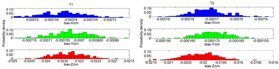
Figure 8.
The frequency histograms of parameter estimator bias.
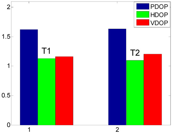
Figure 9.
The average PDOP, HDOP and VDOP for each set of tests.
As is shown in Table 2 and Figure 10, the hypothesis test is implemented to check the parameter estimator bias. The bias of two test points in the coordinate component z is much larger than x and y. Because the anchors are distributed in a plane. It makes known that the positioning configuration is symmetrical in the x and y direction, but it is ill-conditioned in component z. The bias in the coordinate components x and y and the Mahalanobis distance at T1 are larger than that of T2. In the x-y plane, the geometry of T2 is closer to the orthogonal condition with the zero bias. It indicates that the test point T2 and anchors constitute a better positioning geometry. Meanwhile, we can see that the test statistic of two tests are both very small compared with the threshold value. It shows that the bias is small enough to be neglected and the linearized model is a sufficiently approximate for UWB positioning. Figure 11 illustrates the parameter estimators in x-y plane with 95% confidence region. It shows that the systematic error of the parameter estimators of at T1 is greater than T2. It makes known that a good geometry can not only reduce the bias caused by the inaccurate functional model, but also compensates for the systematic error due to the hardware devices used.
Table 2.
The mean parameter estimator bias ( cm).
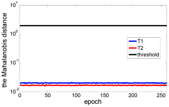
Figure 10.
The hypothesis test based on Mahalanobis distance.
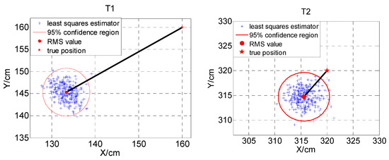
Figure 11.
The location estimation results.
5.2.2. Dynamic Test
The main goal of this test is to evaluate the bias of least-squares parameter estimator in a dynamic situation. The coordinates of anchors are consistent with the static positioning. The test trajectory and the experimental scene are shown in Figure 12. The tester walked along the predetermined trajectory. Besides, an additional set of test analysis is implemented by adding large noise with the standard deviation of 20 cm to the original observations. It stimulates non-line-of-sight (NLOS) environment, the error of measurements increased.
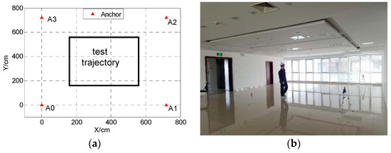
Figure 12.
The test trajectory (a) and the experimental scene (b).
The frequency histograms of parameter estimator bias are shown in Figure 13. Since the anchors and trajectory are all symmetrical in the horizontal direction, the bias in the coordinate components x and y are also basically symmetrical. The bias in the coordinate component z is also greater as before. Besides, since the dynamic motion process on the preset trajectory does not satisfy the orthogonal condition of the design matrix and the bias amount of nonlinearity. The bias in the coordinate components x and y is not unbiased and the probability of large bias in the coordinate components x and y is larger than that of small bias. Furthermore, the bias of all coordinate components in dynamic test with large noise is larger than that of original dynamic test.
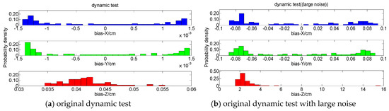
Figure 13.
The frequency histograms of parameter estimator bias.
Moreover, as is shown in Figure 14, the noise will influence the observations, which in turn affects the stability of the system geometry and the calculation of DOP value. Furthermore, these factors together affect the calculation of parameter estimator bias. Figure 15 and Figure 16 demonstrate that the large noise in NLOS environment directly affects the magnitude of the bias in the nonlinear least-squares estimator, and the Mahalanobis distance of many epochs have exceeded the threshold. We can believe that the bias estimate can be used to correct the least-squares estimator to guarantee the unbiasedness for UWB positioning. For the relatively high measurement precision and good positioning configuration, the linearization is valid and the bias can be neglected.
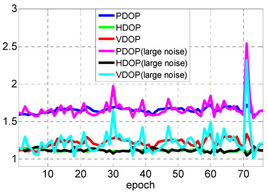
Figure 14.
The average PDOP, HDOP and VDOP for each set of tests.
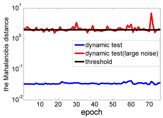
Figure 15.
The hypothesis test based on Mahalanobis distance.
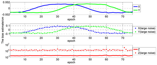
Figure 16.
The bias estimate of two set of tests.
Through the above analysis, we can verify that the bias in the least-squares estimator is driven by the prior precision, the design matrix and the amount of nonlinearity. In some special positioning areas like the emergency services, the localization process acts rapidly in the unknown indoor environments, so it is unrealistic to rely on a pre-existing installation with beforehand measurements, calibration, configuration and deployment. The positioning system may be ill-posed or has large ranging measurement noise. It is necessary to judge the validity of linearized model and to realize the unbiasedness for UWB positioning.
6. Conclusions
The main goal of this paper is to analyze the parameter estimator bias. It provides an overview of the reliability of Gauss–Newton method applied to UWB positioning. The linearization of the positioning functional model result in biased least-squares estimators. The Gauss–Newton method only includes the first-order Taylor expansion of distance equations. The bias comes from neglected higher order terms, which can be regarded as a systematic error. In this paper, we analyze how the second-order partial derivate affect the parameter estimator bias. The parameter estimator bias is related to the system geometry and the observation quality. It is driven by the prior observation precision, the design matrix and the amount of nonlinearity. It will be realized that the parameter estimator tends to be unbiased with a sufficiently small relative ranging error or a good positioning configuration with the lowest DOP. In outdoor satellite positioning, the ranging distances are long enough so that the relative residual are very small. A better positioning geometry configuration also can be chosen thanks to the large number of satellites available. This extremely large system makes the bias totally negligible. However, in the UWB indoor positioning, the ranging distances are extremely short. Meanwhile, the NLOS environment makes the error of measurements increased and biased. In addition, considering the complexity and cost of the positioning system, the geometry configuration of anchor nodes is prone to be ill-conditioned. Thus, it makes the parameter estimator bias significant, and the performance and the reliability of the positioning functional model are inevitably influenced. A judging index for the hypothesis test based on Mahalanobis distance is proposed to determine if the bias is significant. It is essentially to assess whether the linearized model is a sufficient approximation and the bias becomes potential problem for UWB positioning. If the bias is too large, the estimator needs to be corrected to endure the unbiasedness for positioning. In practical applications, an unbiased estimation of the positioning result will be expected, the bias can be calculated by the standard least-squares procedure prior to designing a positioning system. Through detecting the large bias due to the error of functional model, the positioning system can be designed the minimum bias from which the parameters are to be estimated.
Author Contributions
Conceptualization, C.W., J.W. and H.Y.; methodology, C.W., J.W. and H.Y.; writing—original draft, C.W.; writing—review and editing, H.Y., J.W. and T.L. All authors have read and agreed to the published version of the manuscript.
Funding
This work is supported by the National Key Research and Development Program of China (2016YFC0803103).
Acknowledgments
We are very grateful to anonymous reviewers for their constructive comments and suggestions.
Conflicts of Interest
The authors declare no conflicts of interest.
References
- Wang, L.; Li, Z.; Zhao, J.; Zhou, K. Smart Device-Supported BDS/GNSS Real-Time Kinematic Positioning for Sub-Meter-Level Accuracy in Urban Location-Based Services. Sensors 2016, 16, 2201. [Google Scholar] [CrossRef] [PubMed]
- Belakbir, A.; Amghar, M.; Sbiti, N.; Rechiche, A. An Indoor-Outdoor positioning system based on the combination of GPS and UWB sensors. J. Theor. Appl. Inf. Technol. 2014, 25, 301–303. [Google Scholar] [CrossRef]
- Li, X.; Yang, S. The indoor real-time 3D localization algorithm using UWB. In Proceedings of the International Conference on Advanced Mechatronic Systems, Beijing, China, 22–24 August 2015. [Google Scholar] [CrossRef]
- Basiri, A.; Lohan, E.S.; Moore, T.; Winstanley, A.; Peltola, P.; Hill, C.; Amirian, P.; Silva, P.F.E. Indoor location based services challenges, requirements and usability of current solutions. Comput. Sci. Rev. 2017, 24, 1–12. [Google Scholar] [CrossRef]
- Ferreira, A.G.; Fernandes, D.; Catarino, A.P.; Monteiro, J.L. Performance Analysis of ToA-Based Positioning Algorithms for Static and Dynamic Targets with Low Ranging Measurements. Sensors 2017, 17, 1915. [Google Scholar] [CrossRef]
- Alarifi, A.; Al-Salman, A.M.; Alsaleh, M.; Alnafessah, A.; Al-Hadhrami, S.; Al-Ammar, M.A.; Al-Khalifa, H.S. Ultra wideband indoor positioning technologies: Analysis and recent advances. Sensors 2016, 16, 707. [Google Scholar] [CrossRef]
- Dabove, P.; Di Pietra, V.; Piras, M.; Jabbar, A.A.; Kazim, S.A. Indoor positioning using Ultra-wide band (UWB) technologies: Positioning accuracies and sensors’ performances. In Proceedings of the IEEE/ION Position, Location and Navigation Symposium, Monterey, CA, USA, 23–26 April 2018. [Google Scholar] [CrossRef]
- Sakr, M.; Masiero, A.; El-Sheimy, N. Evaluation of Dynamic AD-HOC UWB Indoor Positioning System. In Proceedings of the International Archives of the Photogrammetry, Remote Sensing and Spatial Information Sciences, Beijing, China, 7–10 May 2018. [Google Scholar] [CrossRef]
- Groβwindhager, B.; Stocker, M.; Rath, M.; Boano, C.A.; Römer, K. SnapLoc: An ultra-fast UWB-based indoor localization system for an unlimited number of tags. In Proceedings of the International Conference on Information Processing in Sensor Networks, Montreal, QC, Canada, 16–18 April 2019. [Google Scholar] [CrossRef]
- Guerra, A.; Decarli, N.; Guidi, F.; Dardari, D. Energy sprinklers for passive UWB RFID. In Proceedings of the 2014 IEEE International Conference on Ultra-WideBand, Paris, France, 1–3 September 2014. [Google Scholar] [CrossRef]
- Guidi, F.; Sibille, A.; Roblin, C.; Casadei, V.; Dardari, D. Analysis of UWB tag backscattering and its impact on the detection coverage. IEEE Trans. Antennas Propag. 2014, 62, 4292–4303. [Google Scholar] [CrossRef]
- Dardari, D.; Decarli, N.; Guerra, A.; Guidi, F. The future of ultra-wideband localization in RFID. In Proceedings of the 2016 IEEE International Conference on RFID, Guangdong, China, 21–23 September 2016. [Google Scholar] [CrossRef]
- Monica, S.; Bergenti, F. Hybrid Indoor Localization Using WiFi and UWB Technologies. Electronics 2019, 8, 334. [Google Scholar] [CrossRef]
- Dardari, D.; Conti, A.; Ferner, U.; Giorgetti, A.; Win, M.Z. Ranging with ultrawide bandwidth signals in multipath environments. Proc. IEEE 2009, 97, 404–426. [Google Scholar] [CrossRef]
- Perakis, H.; Gikas, V. Evaluation of range error calibration models for indoor UWB positioning applications. In Proceedings of the International Conference on Indoor Positioning and Indoor Navigation, Nantes, France, 24–27 September 2018. [Google Scholar] [CrossRef]
- Wymeersch, H.; Maranò, S.; Gifford, W.M.; Win, M.Z. A machine learning approach to ranging error mitigation for UWB localization. IEEE Trans. Commun. 2012, 60, 1719–1728. [Google Scholar] [CrossRef]
- Gigl, T.; Janssen, G.J.; Dizdarevic, V.; Witrisal, K.; Irahhauten, Z. Analysis of a UWB indoor positioning system based on received signal strength. In Proceedings of the 4th Workshop on Positioning, Navigation and Communication, Hannover, Germany, 22–22 March 2007. [Google Scholar] [CrossRef]
- Foy, W.H. Position-location solutions by Taylor-series estimation. IEEE Trans. Aerosp. Electron. Syst. 1976, 187–194. [Google Scholar] [CrossRef]
- Awange, J.L.; Fukuda, Y. Resultant optimization of the three-dimensional intersection problem. Surv. Rev. 2007, 39, 100–108. [Google Scholar] [CrossRef]
- Teunissen, P.J.G. Nonlinear least squares. Manuscr. Geod. 1990, 15, 137–150. [Google Scholar]
- Cook, R.D.; Tsai, C.L.; Wei, B.C. Bias in nonlinear regression. Biometrika 1986, 73, 615–623. [Google Scholar] [CrossRef]
- Teunissen, P.J.G. First and second moments of non-linear least-squares estimators. Bull. Géod. 1989, 63, 253–262. [Google Scholar] [CrossRef][Green Version]
- Jeudy, L.M. Generalyzed variance-covariance propagation law formulae and application to explicit least-squares adjustments. Bull. Géod. 1988, 62, 113–124. [Google Scholar] [CrossRef]
- Teunissen, P.J.G. Nonlinear inversion of geodetic and geophysical data: Diagnosing nonlinearity. In Proceedings of the Ron Mather Symposium on Four-Dimensional Geodesy, Sydney, Australia, 28–31 March 1989. [Google Scholar] [CrossRef]
- Teunissen, P.J.G.; Knickmeyer, E.H. Nonlinearity and least-squares. CISM J. ACSGC 1988, 42, 321–330. [Google Scholar] [CrossRef]
- Yan, J.; Tiberius, C.C.J.M.; Bellusci, G.; Janssen, G.J.M. Feasibility of Gauss-Newton method for indoor positioning. In Proceedings of the IEEE Position Location and Navigation Symposium, Monterey, CA, USA, 5–8 May 2008. [Google Scholar] [CrossRef]
- Xue, S.; Yang, Y. Unbiased nonlinear least squares estimations of short-distance equations. J. Navig. 2017, 70, 19. [Google Scholar] [CrossRef]
- Imparato, D.; Teunissen, P.J.G.; Tiberius, C.C.J.M. Minimal detectable and identifiable biases for quality control. Surv. Rev. 2019, 51, 289–299. [Google Scholar] [CrossRef]
- Teunissen, P.J. Distributional theory for the DIA method. J. Geod. 2018, 92, 59–80. [Google Scholar] [CrossRef]
- Zaminpardaz, S.; Teunissen, P.J.G. DIA-datasnooping and identifiability. J. Geod. 2019, 93, 85–101. [Google Scholar] [CrossRef]
- Rofatto, V.F.; Matsuoka, M.T.; Klein, I.; Veronez, M.R.; Bonimani, M.L.; Lehmann, R. A half-century of Baarda’s concept of reliability: A review, new perspectives, and applications. Surv. Rev. 2018, 1–17. [Google Scholar] [CrossRef]
- El-Mowafy, A. Real-Time Precise Point Positioning Using Orbit and Clock Corrections as Quasi-Observations for Improved Detection of Faults. J. Navig. 2017, 71, 769–787. [Google Scholar] [CrossRef]
- El-Mowafy, A. On detection of observation faults in the observation and position domains for positioning of intelligent transport systems. J. Geod. 2019, 1–14. [Google Scholar] [CrossRef]
- Chang, G. Robust Kalman filtering based on Mahalanobis distance as outlier judging criterion. J. Geod. 2014, 88, 391–401. [Google Scholar] [CrossRef]
- Luong, A.; Hillyard, P.; Abrar, A.S.; Che, C.; Rowe, A.; Schmid, T.; Patwari, N. A stitch in time and frequency synchronization saves bandwidth. In Proceedings of the International Conference on Information Processing in Sensor Networks, Porto, Portugal, 11–13 April 2018. [Google Scholar] [CrossRef]
- Jiménez, A.R.; Seco, F. Comparing Decawave and Bespoon UWB location systems: Indoor/outdoor performance analysis. In Proceedings of the International Conference on Indoor Positioning and Indoor Navigation, Alcala de Henares, Spain, 4–7 October 2016. [Google Scholar] [CrossRef]
- Yan, J.; Tiberius, C.C.J.M.; Teunissen, P.J.G.; Bellusci, G.; Janssen, G.J.M. A framework for low complexity least-squares localization with high accuracy. IEEE Trans. Signal. Process. 2010, 58, 4836–4847. [Google Scholar] [CrossRef]
- Izenman, A.J. Modern Multivariate Statistical Techniques; Springer: New York, NY, USA, 2008; ISBN 978-0-387-78189-1. [Google Scholar]
© 2019 by the authors. Licensee MDPI, Basel, Switzerland. This article is an open access article distributed under the terms and conditions of the Creative Commons Attribution (CC BY) license (http://creativecommons.org/licenses/by/4.0/).