Line-Detection Based on the Sum of Gradient Angle Differences

Abstract

This paper presents a method to detect line pixels based on the sum of gradient angle differences (SGAD). The gradient angle differences are calculated by comparing the four pairs of gradients arising from eight neighboring pixels. In addition, a method to classify line pixels into ridges and valleys is proposed. Furthermore, a simple line model is defined for simulation experiments. Experiments are conducted with simulation images generated using the simple line model for three line-detection methods: second-derivatives (SD)-based method, extremity-count (EC)-based method, and proposed method. The results of the simulation experiments show that the proposed method produces more accurate line-detection results than the other methods in terms of the root mean square error when the line width is relatively large. In addition, the experiments conducted with natural images show that the SD- and EC-based methods suffer from bifurcation, fragmentation, and missing pixels. By contrast, for the original and the noise-contaminated versions of the natural images, the proposed SGAD-based line-detection method is affected by such problems to a considerably smaller extent than the other two methods.

1. Introduction

In image-processing terminology, a line is a geometrically elongated feature that is either brighter or darker in intensity than its neighbors on either sides. In some scientific literature, a line is referred to as a ridge or a valley [1,2,3]. As one of the most important and frequently observed features in various types of imagery, including indoor imagery, building facade imagery, satellite imagery, medical imagery, and road imagery, a line is used by perceptual systems to analyze and interpret a scene in an image [4]. Therefore, line detection is a fundamental operation in image processing and computer vision. Another image processing technique called edge detection is used to find the boundaries of objects within images. Various operators are used to detect edges, including Robert’s operator [5], the Sobel operator [6], Prewitt operator [7], Laplacian of Gaussian (LoG) operator followed by zero crossing [8], and Canny operator [9]. These operators have ensured the widespread use of edge detection as an image-processing technique.

Owing to the lack of an efficient direct method, edge-detection results are frequently employed to extract line features [10,11,12,13,14,15]. However, this indirect method often fails to detect lines accurately, especially when the edge signal emanating from a line in an image is weak as compared to noise strength. In addition, this method requires a post-processing step to detect line pixels based on the edge pixels it detected on both sides of the line.

In recent years, the demand for efficient extraction of line features from images has grown rapidly owing to advancements in various applications, including lane detection in autonomous driving [10,11,12,13], blood vessel detection in medical imaging [14,15], and road detection in satellite imaging [16].

Although the demand for a method to detect line features directly has been strong, existing line-detection methods do not satisfy the quality requirements to serve the demand. For high-quality line detection, the operator must be insensitive to noise.

The second-derivatives (SD)-based method for line detection was proposed approximately two decades ago in [17,18]. However, in this paper, for relatively large line widths, the SD-based line-detection method was shown to produce dis-localized line pixels and low SNR. Line detection based on extremity count (EC) was proposed in [4]. However, this method only partially fulfilled the requirements of high-quality line detection. To resolve these problems and achieve high performance, herein, a novel line-detection method based on the sum of gradient angle differences (SGAD) is proposed. Furthermore, the present study proves that the performance of the SGAD-based line-detection method is better than that of the SD- and EC-based line-detection methods and that the proposed method maintains high quality even when the line width is relatively large. The main reason for the high quality of line-detection of the proposed method is the use of the oppositeness of gradient directions between four pairs of neighborhood pixels around a line pixel, which is relatively less affected by high noise level and relatively large line width as compared to other methods, thus providing higher SNR under varying conditions.

The remainder of this paper is organized as follows. Section 2 describes related line-detection studies. Section 3 describes the proposed line-detection method. Section 4 and Section 5 detail the experimental results obtained using simulation images and natural images, respectively. Section 6 concludes this paper.

2. Related Work

As one of the earliest approaches to detecting linear features, Paton [19] proposed a method to detect edge and line pixels. This method was based on the analysis of the coefficients resulting from the fitting of Legendre polynomials of degree two or lower to local intensities, in which a set of combinations of the coefficients was used to classify the pixels into edge, ridge, valley, and other geometric features. Although this approach had the ability to classify a given intensity surface into multiple types, it was majorly limited in terms of line detection because it needed to execute a sequence of steps to detect line pixels and a set of well-tuned threshold values, generating which is an arduous task. Haralick [1] proposed a method to detect ridges and valleys by finding the pixels of zero crossings of the first directional derivatives in the direction that extremizes the second directional derivative function. The method employed 10 coefficients generated by fitting a bivariate cubic polynomial to intensity surfaces within a local window. A drawback of this method was the possibility of the generation of non-trivial ringing artifacts that cannot be removed. In addition, this approach required a large window size to calculate the 10 coefficients of the bivariate cubic polynomial. Moreover, this approach encountered problems when localizing the ridge and valley pixels because the intensity surface tended to deviate from the bivariate cubic polynomial surface model, resulting in a relatively large number of false positives and ringing artifacts. Ghosal and Mehrotra [20] proposed another parameter-based edge- and line-detection method that employed Zernike moments to calculate the parameters of edges and lines.

Gauch and Pizer [2] and Serrat et al. [3] proposed methods to find ridge and valley pixels by using differential geometry, which finds zero crossings of the gradients of the curvature of the level curve. However, these approaches were limited by their high computational cost for calculating the first-, second-, and third-order derivatives of intensity surfaces.

Steger [18] and Lindeberg [17] proposed line-detection approaches that identify line pixels based on large second directional derivatives in a direction determined by the eigenvector corresponding to the maximum absolute eigenvalue of the Hessian matrix. In similar studies, Laptev et al. [21] and Jeon et al. [22] employed Steger¡s method to detect roads in aerial images and synthetic-aperture radar images, respectively. However, as will be demonstrated in the following sections, the SD-based line-detection methods used in the abovementioned studies suffer from problems such as non-unique responses to a single line signal and dis-localization because of a relatively large line width. Lindeberg [17] proposed a multi-scale-based line-detection approach to find line pixels that respond most strongly to multi-scale filter operations. This approach may, however, be limited when used to detect line features located near other non-homogeneous features, which are observed frequently in many types of images. These limitations occur because, at a larger scale, the features in the neighborhood intersperse, causing line signals to mingle and become dis-localized. One solution to this problem is the use of line detection or edge detection when the line width is relatively small or relatively large, respectively.

A simple rapid line-detection method that detects ridge and valley pixels by using EC, which is derived from relational operations, to compare the intensity and other properties of a center pixel with those of neighboring pixels has been proposed in [4]. Although the computational cost of this method is low, its performance is limited, especially when images are contaminated with noise, as will be demonstrated in the following sections. A line-detection method that uses multi-scale anisotropic Gaussian kernels for characterizing the second-order partial derivative of an intensity image was proposed in [23]. However, the characterization requires computation of all responses to varying combinations of filter direction, smoothing factor, and degree of anisotropy, which makes it computationally expensive.

A multi-step-based line-detection approach was proposed in [24]. This approach uses a combination of three filters—oriented elongated filters, multi-scale top-hat, and K-SVD—to detect cracks in paintings. This approach, too, is computationally expensive because it employs a set of elongated filters and multiple steps.

A line-detection method that uses a creaseness measure calculated based on the sum of differences among the gradients of neighboring pixels was proposed in [25]. One of the limitations of this approach is that a simple sum of gradient differences may not be a plausible indicator of the existence of line pixels because each gradient vector loses its directionality when the direct sum of gradient differences is applied. The SGAD approach proposed herein overcomes this limitation by using the value derived by adding the absolute values of the differences of four pair of gradient vector directions, where the vector pair is made by each of a set of four predefined directions.

Regarding the evaluation of line-detection methods, Zwiggelaar et al. [26] compared the performance of several line detectors for medical images based on receiver operating characteristic curves. In addition, Lopez et al. [25] evaluated several ridge- and valley-detection methods by using various types of images.

3. Proposed Line-Detection Method

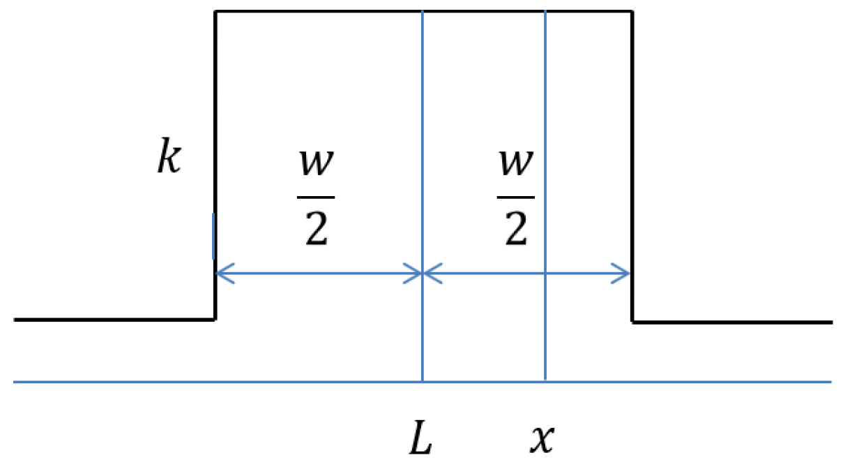
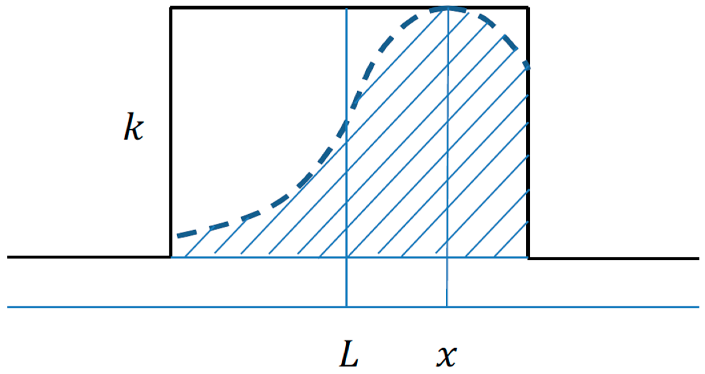
In this section, a line-detection method based on SGAD is proposed. First, the line model is introduced. Then, SGAD is defined.

3.1. Line Model

In image processing, blur and noise are always non-negligible because of the limitations of camera lens systems. Studies have previously adopted the approach that any real image $\mathbf{I}$ can be modeled as a base signal $\mathbf{F}$ convolved with blur $\mathbf{b}$ and noise $\mathbf{n}$ [27,28,29,30,31,32,33,34,35], as follows:

$$\mathbf{I}=\mathbf{F}\ast \mathbf{b}+\mathbf{n},$$

(1)

where ∗ represents the convolution operator. Although a more complete blur model with blurring patterns in edge neighborhoods was proposed in [36], the present study employed the image formation model described in (1) for simplifying experiments.

In this study, line profile is modeled in terms of width w and contrast k, as shown in Figure 1. Although a more general line model has been proposed previously [18], which models a line with different contrasts on either side, the derivation here uses the simpler model shown in Figure 1 because it simplifies subsequent tests, and most line features have similar contrasts on either side.

From Figure 1, the one-dimensional line signal is modeled as follows:

$$\mathbf{F}\left(x\right)=\left\{\begin{array}{cc}h+k,\hfill & \mathrm{if}|x-L|<\frac{w}{2};\hfill \\ h,\hfill & \mathrm{otherwise}\hfill \end{array}\right.,$$

(2)

where L is the coordinate of the line center.

The following one-dimensional Gaussian blur is introduced to consider the blur effects that occur during image formation:

$$\mathbf{b}\left(t\right)=\frac{1}{\sqrt{2\pi }{\sigma }_b}{e}^{-\frac{t^2}{2{\sigma }_b^2}},$$

(3)

where ${\sigma }_b$ is the blurring factor.

Figure 2 shows an exaggerated version of the blur function $k·\exp (-\frac{{(t-x)}^2}{2{\sigma }_b^2})$ centered at an arbitrary location x. Thus, the intensity at x after blurring is given as follows:

$$\begin{array}{cc}\hfill {\mathbf{F}}_{\mathbf{b}}\left(x\right)=& (\mathbf{F}\ast \mathbf{b})\left(x\right)={\int }_{x-\frac{w}{2}-L}^{x+\frac{w}{2}-L}\frac{k}{{\sigma }_b\sqrt{2\pi }}{e}^{-\frac{t^2}{2{\sigma }_b^2}}dt,\hfill \\ \hfill =& \frac{k}{2}\left[\mathrm{erf}\left(\frac{x+\frac{w}{2}-L}{{\sigma }_b\sqrt{2}}\right)-\mathrm{erf}\left(\frac{x-\frac{w}{2}-L}{{\sigma }_b\sqrt{2}}\right)\right],\hfill \end{array}$$

(4)

where $\mathrm{erf}(·)$ is the error function.

For denoising, a certain amount of smoothing is invariably required. Image smoothing is typically performed with a kernel defined by a two-dimensional Gaussian function, which can be described as follows:

$$\mathbf{s}(u,v)=\frac{1}{2\pi {\sigma }_s^2}{e}^{-\frac{u^2+v^2}{2{\sigma }_s^2}},$$

(5)

where ${\sigma }_s$ is the smoothing factor. The corresponding one-dimensional smoothing function can be written as follows:

$$\mathbf{s}\left(u\right)=\frac{1}{\sqrt{2\pi }{\sigma }_s}{e}^{-\frac{u^2}{2{\sigma }_s^2}}.$$

(6)

Then, by applying the convolution of the smoothing function $\mathbf{s}$ to the original image, the smoothed image ${\mathbf{I}}_{\mathbf{s}}$ can be generated as follows:

$${\mathbf{I}}_{\mathbf{s}}=\mathbf{I}\ast \mathbf{s}=(\mathbf{F}\ast \mathbf{b}+\mathbf{n})\ast \mathbf{s}=\mathbf{F}\ast \mathbf{b}\ast \mathbf{s}+\mathbf{n}\ast \mathbf{s}.$$

(7)

Thus, after the convolutions of blurring and smoothing, the original line signal in (2) is transformed according to [37] as follows:

$${\mathbf{F}}_{\mathbf{b}\ast \mathbf{s}}\left(x\right)=(\mathbf{F}\ast \mathbf{b}\ast \mathbf{s})\left(x\right)=({\mathbf{F}}_{\mathbf{b}}\ast \mathbf{s})\left(x\right)={\int }_{x-\frac{w}{2}-L}^{x+\frac{w}{2}-L}\frac{k}{\sqrt{2\pi ({\sigma }_b^2+{\sigma }_s^2)}}{e}^{-\frac{t^2}{2({\sigma }_b^2+{\sigma }_s^2)}}dt.$$

(8)

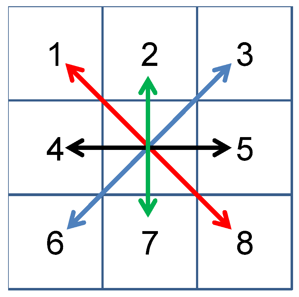
3.2. Definition of SGAD

First, the gradient angle at each pixel is calculated as follows:

$${\theta }_i={\tan }^{-1}\left(\frac{g_{r_i}}{g_{c_i}}\right),$$

(9)

where $g_{r_i}$ and $g_{c_i}$ are the gradients of the smoothed intensities in (7) at pixel i in the row and column directions, respectively, as follows:

$$g_{r_i}=\frac{\partial {\mathbf{I}}_{\mathbf{s}}}{\partial r}\left(i\right)\mathrm{and}{g}_{c_i}=\frac{\partial {\mathbf{I}}_{\mathbf{s}}}{\partial c}\left(i\right),$$

(10)

where r and c are row and column coordinates, respectively.

Then, the difference between the gradient angles of two pixels is calculated by finding the minimum positive angle between the gradient vectors at the two pixels as follows:

$${\delta }_{i,j}=\min \left(\mathrm{abs}\left({\theta }_i-{\theta }_j\right),2\pi -\mathrm{abs}\left({\theta }_i-{\theta }_j\right)\right).$$

(11)

The difference in angles is calculated for four pairs of gradient vectors, as shown in Figure 3. The angle differences of the four pairs are summed to generate the SGAD measure, as follows:

$$\mathrm{SGAD}={\delta }_{1,8}+{\delta }_{2,7}+{\delta }_{3,6}+{\delta }_{4,5}.$$

(12)

3.3. Classification of Line Pixels into Ridge and Valley, and Suppression of Non-Maxima

The pixels classified as line pixels in the previous step are further classified into the groups ridge and valley. A ridge is a line feature with an intensity greater than that of other features in its neighborhood, and a valley is a line feature with an intensity lower than that of the other features in its neighborhood. The aforementioned classification is based on the sum of the convolutions of the gradients with the following two kernels. The first kernel is defined as follows:

$${\mathbf{N}}_{\mathbf{c}}=\left[\begin{array}{ccc}-1& 0& 1\\ -1& 0& 1\\ -1& 0& 1\end{array}\right].$$

(13)

The second kernel is defined as follows:

$${\mathbf{N}}_{\mathbf{r}}=\left[\begin{array}{ccc}-1& -1& -1\\ 0& 0& 0\\ 1& 1& 1\end{array}\right].$$

(14)

$N_c$ in (13) gathers gradients outgoing from (or incoming to) the center of the kernel in the column direction. Similarly, $N_r$ in (14) gathers gradients outgoing from (or incoming to) the center of the kernel in the row direction.

The measure that indicates whether a line pixel at (r,c) is a ridge or a valley is calculated as follows:

$$\mathrm{RV}(r,c)=-\left[({\mathbf{g}}_{\mathbf{r}}\ast {\mathbf{N}}_{\mathbf{r}})+({\mathbf{g}}_{\mathbf{c}}\ast {\mathbf{N}}_{\mathbf{c}})\right](r,c),$$

(15)

where ${\mathbf{g}}_{\mathbf{r}}$ and ${\mathbf{g}}_{\mathbf{c}}$ denote images containing the gradients in the row and the column directions, respectively. If $\mathrm{RV}(r,c)$ is positive, the pixel at (r,c) is classified as ridge. Else, the pixel is classified as valley.

Then, a non-maxima suppression process is employed to eliminate the detected line pixels whose absolute SGAD values are non-maxima as compared to those of their neighboring pixels. The suppression process is executed using only the neighboring pixels of the same line class, with either ridge or valley as the center pixel. In addition, the suppression process employs the maximum curvature direction, which is determined from the eigenvector corresponding to the maximum eigenvalue of the Hessian matrix [18].

4. Line-Detection Experiments with Simulated Images

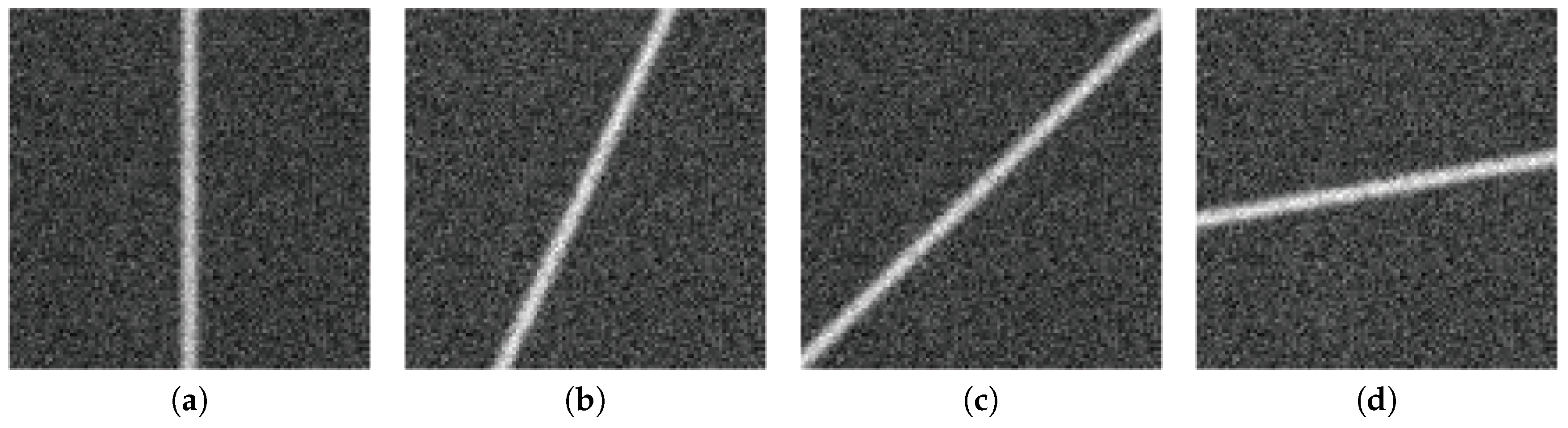
4.1. Generation of Simulated Images

To test the line-detection performance of the SD-, EC-, and proposed SGAD-based methods, a series of images was generated containing line features with fixed blurring factor ${\sigma }_b=1$, varying line width w, line normal angle $\theta$, and noise ${\sigma }_n$. For the given image center coordinates $(r_o,c_o)$ and line normal direction $\theta$, normal distance from the origin to the center of the line $\rho$ was calculated as follows:

$$\rho =c_{o}cos\theta +r_{o}sin\theta ,$$

(16)

and the following two metrics were calculated for each pixel location $(r,c)$.

$$\begin{array}{cc}\hfill D_1(r,c)=& \frac{ccos\theta +rsin\theta -\rho +\frac{w}{2}}{{\sigma }_b\sqrt{2}}\hfill \\ \hfill D_2(r,c)=& \frac{ccos\theta +rsin\theta -\rho -\frac{w}{2}}{{\sigma }_b\sqrt{2}}.\hfill \end{array}$$

(17)

For the given contrast k, described in (2), the intensity at each pixel was then calculated according to (4) as

$${\mathbf{F}}_{\mathbf{b}}(r,c)=\frac{k}{2}\left[\mathrm{erf}\left(D_1(r,c)\right)-\mathrm{erf}\left(D_2(r,c)\right)\right].$$

(18)

An image was generated by adding a noise image $\mathbf{n}$, as follows:

$$\mathbf{I}={\mathbf{F}}_{\mathbf{b}}+\mathbf{n},$$

(19)

where $\mathbf{n}(r,c)$ was assumed to follow the normal distribution $N(0,{\sigma }_n^2)$.

Figure 4 shows four typical examples of $101\times 101$ pixel simulation line images with varying $\theta$ and constant $k=1$, ${\sigma }_b=1$, $w=4$, and ${\sigma }_n=30/255$.

Denoising is commonly applied before feature extraction from noise-contaminated images to ensure that the extracted features are of the highest possible quality. Therefore, in the present study, the following smoothing convolution is applied:

$${\mathbf{I}}_{\mathbf{s}}=\mathbf{I}\ast \mathbf{s},$$

(20)

where $\mathbf{s}$ is a two-dimensional Gaussian function with standard deviation ${\sigma }_s$.

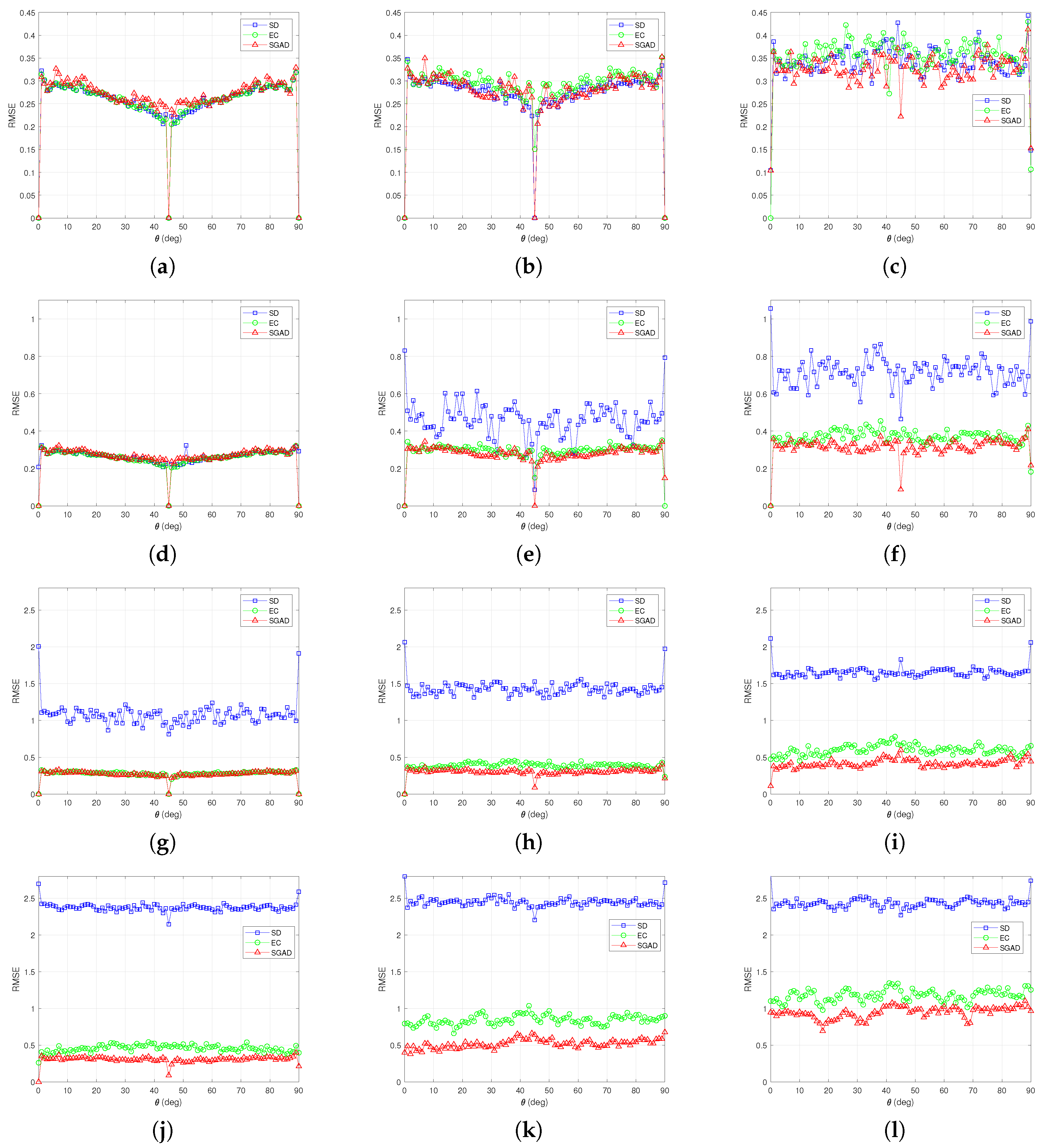
4.2. Special Simulation Tests

In the experiments conducted with the simulation images, line pixels were detected using the SD-, EC-, and SGAD-based methods from the pixels located within half of each line width from the true center lines of the simulation line features. For implementing the SD-based method, SD values at the pixels were calculated, and the pixels were classified as ridge or valley according to their $RV$ values calculated using (15). Then, non-maxima suppression was applied to the image containing the SD values, as described in Section 3.3, where SD values were used instead of SGAD values. The experiment with the SGAD-based method followed the procedure described in Section 3. The only parameter to be set for implementing SGAD is the SGAD threshold. In the present study, the threshold value was set to $\pi$. Thus, line pixels were detected when the SGAD value was greater than $\pi$. Experiments with the EC-based method counted the cases of maximum and minimum of each pixel as compared to the intensities of its neighborhood pixels in four pairs of directions. Further, if the count of the number of maximum or minimum cases of each pixel was greater than or equal to 2, the pixel was classified as ridge or valley, respectively. Thus, the EC-based method classified certain pixels as both ridge and valley. Non-maxima suppression was not applied to the EC images in the EC-based method because EC is not a good measure for non-maxima suppression.

Figure 5 shows the typical line-detection results obtained with varying ${\sigma }_n$, w, and $\theta$. As shown in Figure 5a–c, the SD-, EC-, and SGAD-based methods produce accurate line-detection results for ${\sigma }_n=10/255$, $w=2$, and $\theta ={30}^{\circ }$. However, as shown in Figure 5d–l, the EC- and SGAD-based methods produce more accurate line-detection results than the SD-based method. Furthermore, as shown in Figure 5g,j, the SD-based method bifurcates the line location when $w=8$. By contrast, as shown in Figure 5h,i,k,l, the EC- and SGAD-based methods are not affected by the bifurcation problem. Based on a detailed comparison of the performance of the EC- and SGAD-based methods, according to Figure 5e,f,h,i,k,l, the SGAD-based method produces more accurate line-detection results than the EC-based method in terms of the detected line locations and the number of fragmentations.

Figure 6 compares the performance of the SD-, EC-, and SGAD-based methods in terms of the root mean square error (RMSE) of the detected positions for varying $\theta$, w, and ${\sigma }_n$. The graphs have different scales depending on w. However, the graphs for $w=6$ and $w=8$ have the same scale.

As shown in Figure 6a–d, the performance of the SD-, EC-, and SGAD-based methods are comparable for $w=2$ with ${\sigma }_n=10/255,30/255,$ and $60/255$ and for $w=4$ with ${\sigma }_n=10/255$. However, as shown in the rest of the panels of Figure 6, the SD-based method yielded line-detection results with RMSEs greater than those of the results yielded by the EC- and SGAD-based methods. This limitation of the SD-based method is ascribed to bifurcation of the SD values when the line width is relatively large. In addition, in a comparison of the EC- and SGAD-based methods, shown in Figure 6a–e,g, the line-detection performances of the two methods are comparable for $w=2,4,6$ with ${\sigma }_n=10/255$; for $w=2,4$ with ${\sigma }_n=30/255$; and for $w=2$ with ${\sigma }_n=60/255$. However, as shown in the other panels of Figure 6, the performance of the SGAD-based method is better than that of the EC-based method in terms of the RMSEs of the detected line pixel locations.

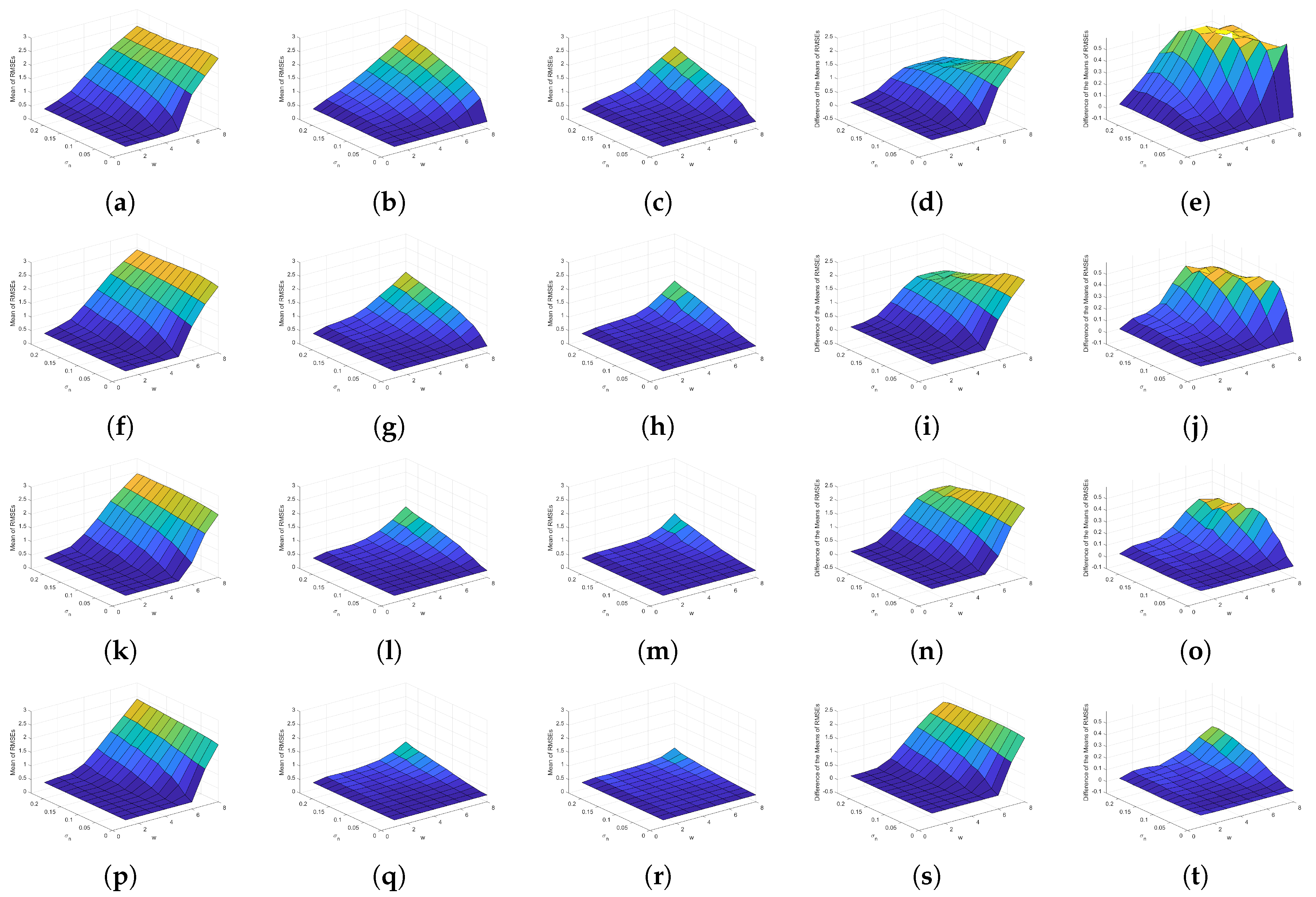
4.3. General Simulation Tests

Tests were performed on simulated line images generated with $w=1,2,\cdots ,8$ and ${\sigma }_n=0,5,\cdots ,60/255$, with $\theta =0,1,\cdots ,{90}^{\circ }$ for each case. Line detection was performed using the SD-, EC-, and SGAD-based methods, and RMSE was then calculated for each case. Finally, mean RMSE was calculated for each combination of w and ${\sigma }_n$. In addition, the effect of smoothing on localization was investigated by setting ${\sigma }_s=0.5,0.75,\cdots ,1.25$; values of ${\sigma }_s>1.25$ were not considered because larger ${\sigma }_s$ values tend to cause signal mixing within a neighborhood in real images and are therefore inappropriate for extracting fine features from images.

Figure 7 shows the outcomes of the experiments conducted on the simulated images with various values of w, ${\sigma }_n$, $\theta$, and ${\sigma }_s$. Overall, SGAD produces more accurate line-detection results than the SD- and the SGAD-based methods under varying w and ${\sigma }_n$. The three methods suffer from large line-detection errors when w is relatively large. However, as shown in columns 4 and 5 of Figure 7, the SGAD-based method produces more accurate line-detection results than the SD- and the EC-based methods when the line width is greater than 3 pixels. Line-detection RMSEs of the three methods increase monotonically with increasing ${\sigma }_n$, but the increase is significantly less for the SGAD-based method compared to those for the SD- and the EC-based methods. Thus, in terms of line-detection performance, the SGAD-based method is more accurate and less sensitive to noise and signal strength than the SD- and the EC-based methods.

Table 1. Processing times of SD-, EC-, and SGAD-based methods for simulated images (in seconds).

${\mathit{\sigma }}_{\mathit{s}}$	SD	EC	SGAD
0.50	31.7	10.2	21.0
0.75	30.5	9.5	19.5
1.00	31.8	9.3	18.6
1.25	30.9	9.0	18.2

summarizes the processing times of the SD-, EC-, and SGAD-based line-detection methods for the simulated images. The three methods were implemented in the MATLAB software environment on a 64-bit PC equipped with an Intel Core I7 Dual CPU and 16 GB RAM. As summarized in Table 1, the SGAD-based method is faster than the SD-based method by more than 30 %. Although the EC-based method was shown to be the fastest among the three methods, the quality of its line-detection results was inferior to that of the SGAD-based method, as will be shown in Section 5. The procedure of the proposed method is composed of two phases. The first phase comprises of smoothing convolution with a Gaussian filter and calculation of the gradients at all pixels in an image. The second phase comprises of calculation of the second derivatives, the SGAD, and the maximum curvature direction, classification of pixels into ridge and valley, and non-maxima suppression at all candidate line pixels. Thus, the computational complexity of the first and second phases of the proposed method are linearly proportional to the number of image pixels and candidate line pixels, respectively.

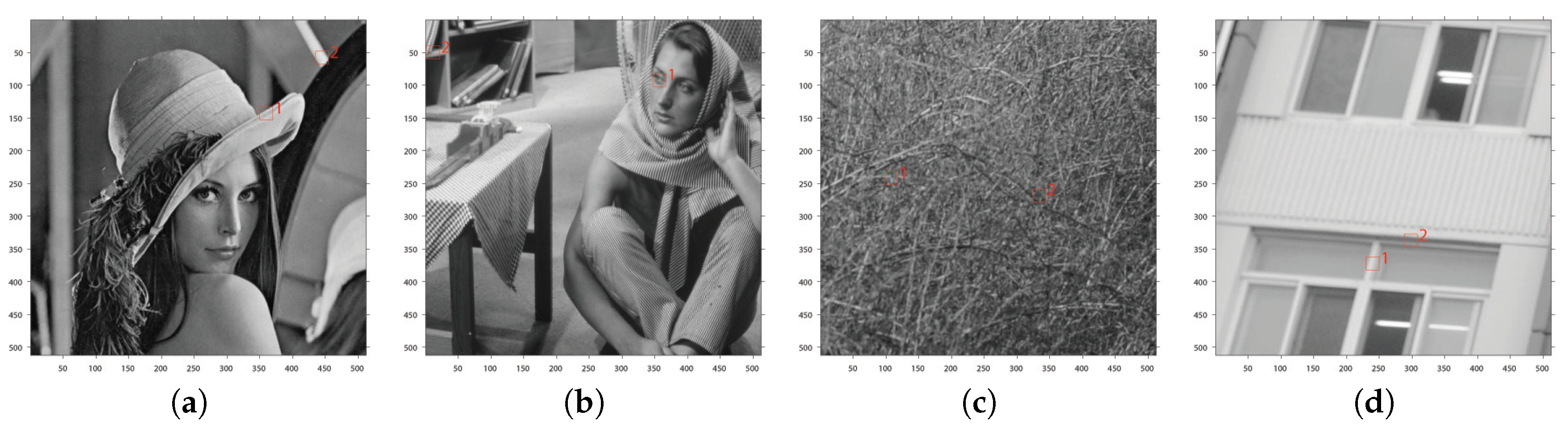
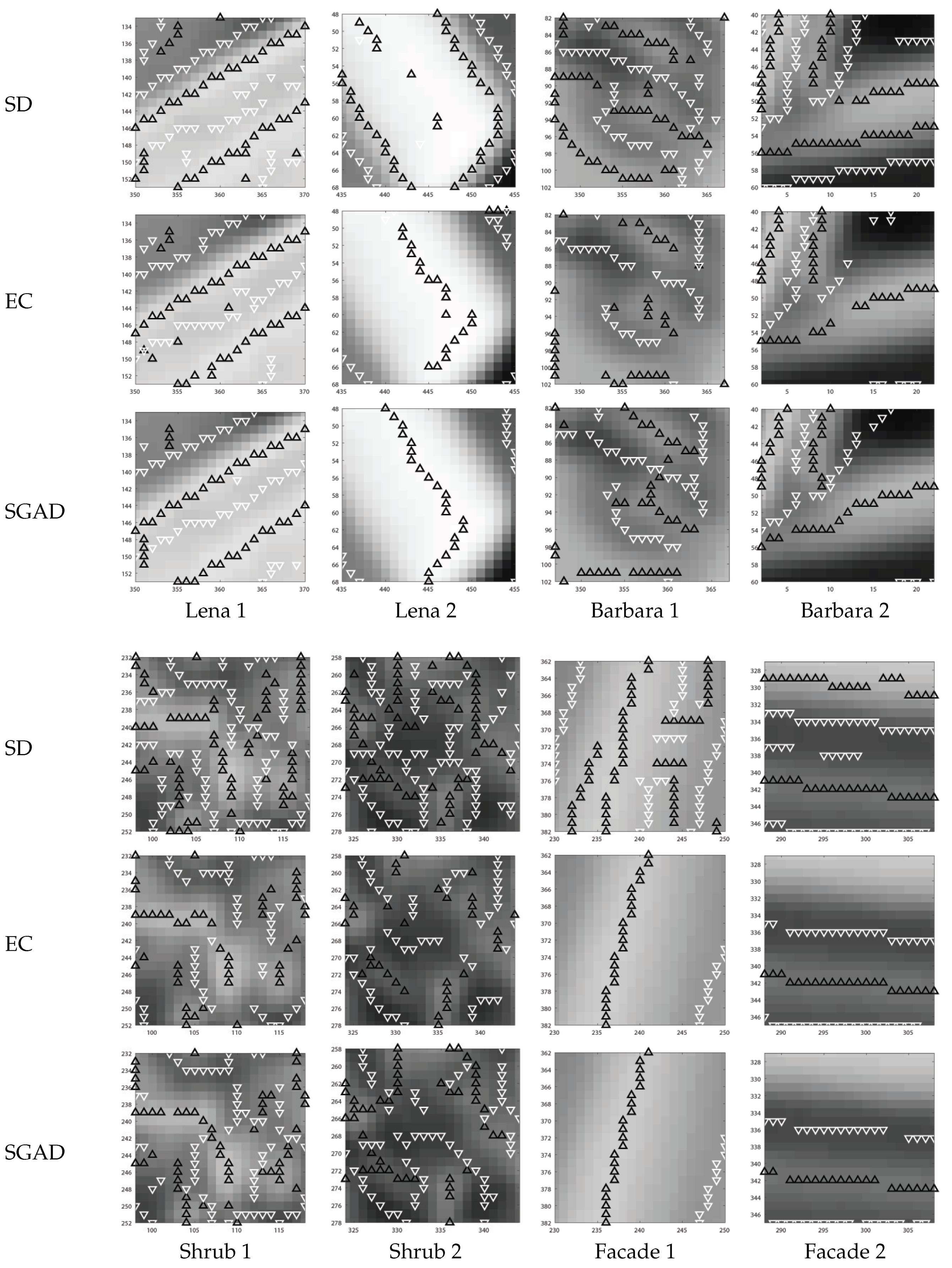
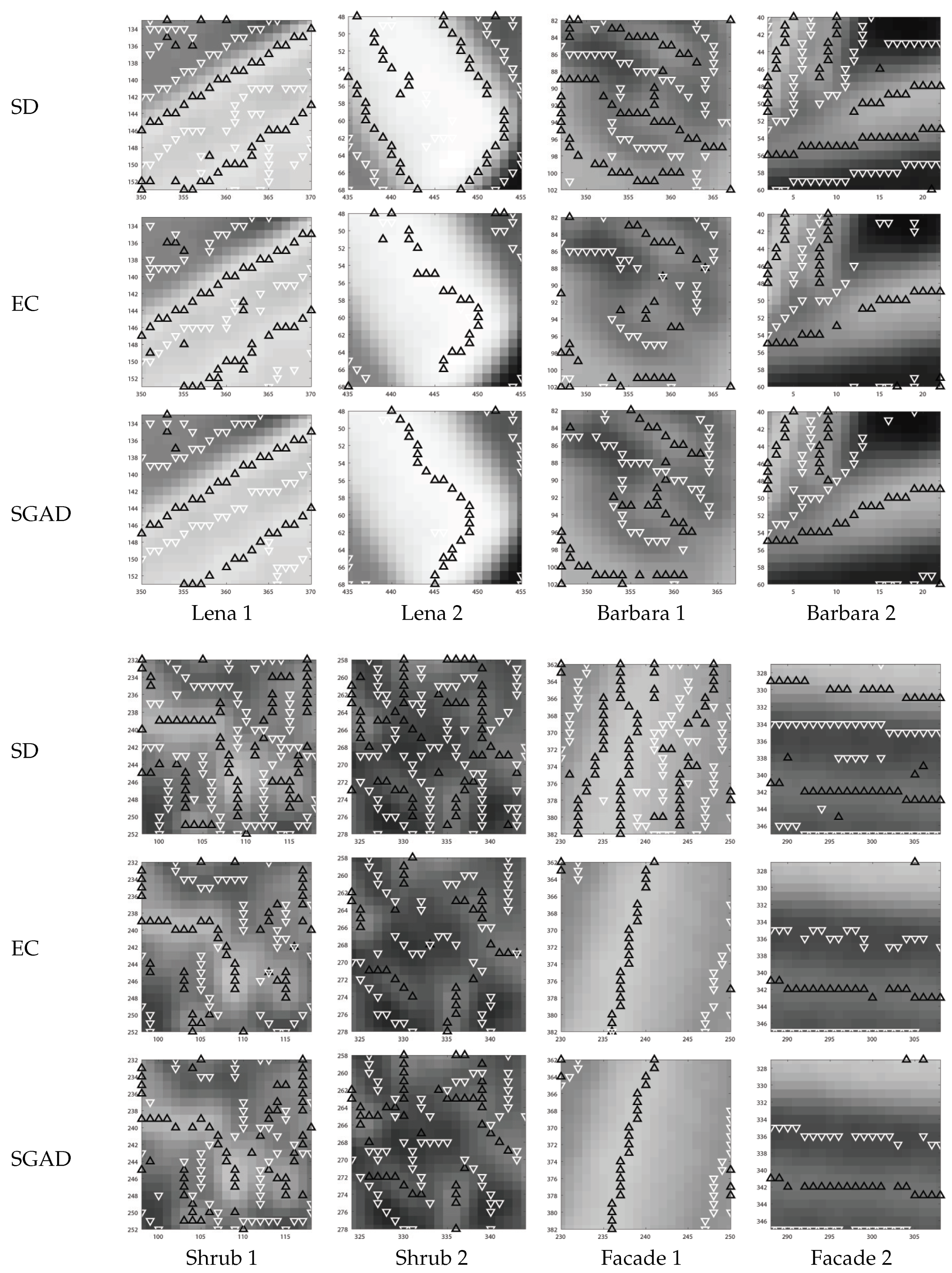
5. Line-Detection Experiments with Natural Images

Figure 8 shows the four $512\times 512$ pixel natural images employed herein. Two of them are the well-known Lena and Barbara images, and the other two are subsets of images of a shrub and a building facade acquired with a DSLR camera. Image intensity was [0, 255].

The performance of the SD-, EC-, and SGAD-based methods was tested in two phases. In the first phase, the performance of the methods was tested using raw images to evaluate their line-detection performance on the original versions of images. In the second phase, the performance of the methods was tested by contaminating the raw images with Gaussian noise ${\sigma }_n=5$.

In both phases, the images were smoothed with ${\sigma }_s=1.0$ to reduce the noise. Figure 9 and Figure 10 show the line-detection results obtained in the first and the second phases for the regions marked by red boxes in Figure 8, respectively. For each natural image, the detailed views of line-detection results for the regions are shown in Figure 9. Figure 10 shows the detailed views of the line-detection results corresponding to those shown in Figure 9.

As shown in Figure 9, the SD-based line-detection method fails to detect the line pixels correctly when line width is relatively large, as shown distinctively in the detailed views of Lena 1, Lena 2, Barbara 2, Facade 1, and Facade 2. In the detailed view of Lena 2, the SD-based method produced the boundary pixels of a thick line feature as line pixels, which is unsuitable given the purpose of line detection.

The EC-based method detected line pixels with a few missing pixels, fragmentation, and a greater number of noisy pixels as compared to the SGAD-based method, as shown in all corresponding detailed views of the results obtained using the EC- and the SGAD-based methods.

Thus, the experimental results obtained using the raw images indicate that the SGAD-based method produces the best line-detection results among the three methods.

As shown in the detailed views of Lena 2 and Facade 2 in Figure 10, the EC-based method is affected by additional noise to a greater extent than the SGAD-based method. The detailed view of Facade 2 shows that the line pixels detected by the EC-based method are more jagged because of the addition of noise than those detected by the SGAD-based method. Thus, the experiments with noisy images indicate that the proposed SGAD-based method is less sensitive to noise compared to the other methods.

6. Conclusions

The proposed SGAD-based line-detection method was proved to produce more accurate line-detection results than the SD- and the EC-based methods by means of experiments conducted using simulation images and natural images.

Implementation of the proposed SGAD-based line-detection method was shown to be simple but less sensitive to noise compared to the other state-of-the-art methods. Thus, the proposed method can be applied readily in general line-detection applications without difficulty because of its simplicity. The SGAD-based line-detection method is expected to provide high-quality line features in applications in the fields of photogrammetry and image processing, such as lane detection, building feature detection, and other applications involving the detection of line features from images.

As the performance of line-detection is dependent on the contrast present in images, a well-designed contrast enhancement process as a pre-processing step [38] can be utilized to improve the quality of the proposed line-detection method.

References

1. Haralick, R.M. Ridges and valleys on digital images. Comput. Vis. Graph. Image Process. 1983, 22, 28–38. [Google Scholar] [CrossRef]
2. Gauch, J.M.; Pizer, S.M. Multiresolution analysis of ridges and valleys in grey-scale images. IEEE Trans. Pattern Anal. Mach. Intell. 1993, 15, 635–646. [Google Scholar] [CrossRef]
3. Serrat, J.; Lopez, A.; Lloret, D. On ridges and valleys. In Proceedings of the 15th International Conference on Pattern Recognition, Barcelona, Spain, 3–7 September 2000. [Google Scholar]
4. Rashe, C. Rapid contour detection for image classification. IET Image Process. 2018, 12, 532–538. [Google Scholar] [CrossRef]
5. Roberts, L. Machine perception of three-dimensional solids. In Optical and Electro-Optical Information Processing; Tippet, J., Berkowitz, D., Clapp, L.C., Koester, C.J., Alexander Vanderburgh, J., Eds.; MIT Press: Cambridge, MA, USA, 1965; pp. 159–197. [Google Scholar]
6. Pingle, K. Visual perception by computer. In Automatic Interpretation and Classification of Images; Grasselli, A., Ed.; Academic Press: New York, NY, USA, 1969; pp. 277–284. [Google Scholar]
7. Prewitt, J. Object enhancement and extraction. In Picture Processing and Psychophysics; Rosenfeld, A., Lipkin, B., Eds.; Academic Press: New York, NY, USA, 1970; pp. 75–149. [Google Scholar]
8. Marr, D.; Hildreth, E. Theory of edge detection. Proc. R. Soc. Lond. 1980, 207, 187–217. [Google Scholar]
9. Canny, J. A computational approach to edge detection. IEEE Trans. Pattern Anal. Mach. Intell. 1986, PAMI-8, 679–698. [Google Scholar] [CrossRef]
10. Jung, C.; Kelber, C. Lane following and lane departure using a linear-parabolic model. Image Vis. Comput. 2005, 23, 1192–1202. [Google Scholar] [CrossRef]
11. An, X.; Shang, E.; Song, J.; Li, J.; He, H. Real-time lane departure warning system based on a single fpga. EURASIP J. Image Video Process. 2013, 38, 1–18. [Google Scholar] [CrossRef] [Green Version]
12. Wu, P.; Chang, C.; Lin, C. Lane mark extraction for automobiles under complex conditions. Pattern Recognit. 2014, 47, 2756–2767. [Google Scholar] [CrossRef]
13. Son, J.; Yoo, H.; Kim, S.; Sohn, K. Real-time illumination invariant lane detection for lane departure warning system. Expert Syst. Appl. 2015, 42, 1816–1824. [Google Scholar] [CrossRef]
14. Karasulu, B. Automatic extraction of retinal blood vessels: A software implementation. Eur. Sci. J. 2012, 8, 47–57. [Google Scholar]
15. Majumdar, J.; Kundu, D.; Tewary, S.; Ghosh, S.; Chakraborty, S.; Gupta, S. An automated graphical user interface based system for the extraction of retinal blood vessels using Kirsch’s template. Int. J. Adv. Comput. Sci. Appl. 2015, 6, 86–93. [Google Scholar] [CrossRef] [Green Version]
16. Wang, W.; Yang, N.; Zhang, Y.; Wang, F.; Cao, T.; Eklund, P. A review of road extraction from remote sensing images. J. Traffic Transp. Eng. 2016, 3, 271–282. [Google Scholar] [CrossRef] [Green Version]
17. Lindeberg, T. Edge detection and ridge detection with automatic scale selection. Int. J. Comput. Vis. 1998, 30, 117–154. [Google Scholar] [CrossRef]
18. Steger, C. An unbiased detector of curvilinear structures. IEEE Trans. Pattern Anal. Mach. Intell. 1998, 20, 113–125. [Google Scholar] [CrossRef] [Green Version]
19. Paton, K. Picture description using Legendre polynomials. Comput. Graph. Image Process. 1975, 4, 40–54. [Google Scholar] [CrossRef]
20. Ghosal, S.; Mehrotra, R. Detection of comosite edges. IEEE Trans. Image Process. 1994, 3, 14–25. [Google Scholar] [CrossRef]
21. Laptev, I.; Mayer, H.; Lindeberg, T.; Eckstein, W.; Steger, C.; Baumgartner, A. Automatic extraction of roads from aerial images based on scale space and snakes. Mach. Vis. Appl. 2000, 12, 23–31. [Google Scholar] [CrossRef] [Green Version]
22. Jeon, B.K.; Jang, J.H.; Hong, K.S. Road detection in spaceborne SAR images using a genetic algorithm. IEEE Trans. Geosci. Remote. Sens. 2002, 40, 22–29. [Google Scholar] [CrossRef]
23. Lopez-Molina, C.; de Ulzurrun, G.V.D.; Baetens, J.; den Bulcke, J.V.; Baets, B.D. Unsupervised ridge detection using second order anisotropic Gaussian kernels. Signal Process. 2015, 116, 55–67. [Google Scholar] [CrossRef]
24. Cornelis, B.; Ruzic, T.; Gezels, E.; Doomes, A.; Pizurica, A.; Platisa, L.; Cornelis, J.; Martens, M.; Mey, M.D.; Daubechies, I. Crack detection and impainting for virtual restoration of paintings: The case of the Ghent Altarpiece. Signal Process. 2013, 93, 605–619. [Google Scholar] [CrossRef]
25. Lopez, A.M.; Lumbreras, F.; Serrat, J.; Villanueva, J.J. Evaluation of methods for ridge and valley detection. IEEE Trans. Pattern Anal. Mach. Intell. 1999, 21, 327–335. [Google Scholar] [CrossRef] [Green Version]
26. Zwiggelaar, R.; Astely, S.M.; Boggis, C.R.M.; Taylor, C.J. Linear structures in mammographic images: Detection and classification. IEEE Trans. Med Imaging 2004, 23, 1077–1086. [Google Scholar] [CrossRef] [PubMed]
27. Lagendijk, R.L.; Tekalp, A.M.; Biemond, J. Maximum likelihood image and blur identification: A unifying approach. Opt. Eng. 1990, 29, 422–435. [Google Scholar]
28. Reeves, S.J.; Mersereau, R.M. Blur identification by the method of generalized cross-validation. IEEE Trans. Image Process. 1992, 1, 301–311. [Google Scholar] [CrossRef] [PubMed]
29. Savakis, A.E.; Trussell, H.J. Blur identification by residual spectral matching. IEEE Trans. Image Process. 1993, 2, 141–151. [Google Scholar] [CrossRef] [Green Version]
30. Kundur, D.; Hatzinakos, D. Blind image deconvolution. IEEE Signal Process. Mag. 1996, 13, 43–64. [Google Scholar] [CrossRef] [Green Version]
31. Yitzhaky, Y.; Kopeika, N.S. Identification of blur parameters from motion blurred images. Graph. Model. Image Process. 1997, 59, 310–320. [Google Scholar] [CrossRef] [Green Version]
32. Chen, L.; Yap, K.H. Efficient discrete spatial techniques for blur support identification in blind image deconvolution. IEEE Trans. Signal Process. 2006, 54, 1557–1562. [Google Scholar] [CrossRef]
33. Wu, S.; Lin, W.; Xie, S.; Lu, Z.; Ong, E.P.; Yao, S. Blind blur assessment for vision-based applications. J. Vis. Commun. Image Represent. 2009, 20, 231–241. [Google Scholar] [CrossRef]
34. Hu, W.; Xue, J.; Zheng, N. PSF estimation via gradient domain correlation. IEEE Trans. Image Process. 2012, 21, 386–392. [Google Scholar] [CrossRef]
35. Liu, S.; Wang, H.; Wang, J.; Cho, S.; Pan, C. Automatic blur-kernel-size estimation for motion deblurring. Vis. Comput. 2015, 31, 733–746. [Google Scholar] [CrossRef]
36. Seo, S. Edge modeling by two blur parameters in varying contrasts. IEEE Trans. Image Process. 2018, 27, 2701–2714. [Google Scholar] [CrossRef] [PubMed]
37. Bromiley, P.A. Products and Convolutions of Gaussian Probability Density Functions; TINA: Manchester, UK, 2018. [Google Scholar]
38. Versaci, M.; Morabito, F.C.; Angiulli, G. Adaptive image contrast enhancement by computing distances into a 4-Dimensional fuzzy unit hypercube. IEEE Access 2017, 5, 26922–26931. [Google Scholar] [CrossRef]
Figure 1. One-dimensional line profile model used in current study.
Applsci 10 00254 g001
Figure 2. Gaussian blur for one-dimensional line model.
Applsci 10 00254 g002
Figure 3. Pairings for calculating gradient angle difference.
Applsci 10 00254 g003
Figure 4. Simulated 101 × 101 pixel images generated with constant contrast ( k = 1 ), line width ( w = 4 ), and noise strength ( σ n = 30 / 255 ) for (a) θ = 0 ; (b) θ = 25 ; (c) θ = 46 ; and (d) θ = 80 .
Applsci 10 00254 g004
Figure 5. Detection results of second-derivatives (SD)-, extremity-count (EC)-, and sum of gradient angle differences (SGAD)-based methods for simulated images with (ac) noise strength σ n = 10 / 255 , line width w = 2 , and line normal angle θ = 30 ; (df) σ n = 30 / 255 , w = 6 , and θ = 25 ; (gi) σ n = 30 / 255 , w = 8 , and θ = 75 ; and (jl) σ n = 60 / 255 , w = 8 , and θ = 15 . (column 1) SD-, (column 2) EC-, and (column 3) SGAD-based line-detection approaches. The red lines indicate the true center lines of the simulated line features.
Applsci 10 00254 g005
Figure 6. Root mean square errors (RMSEs) of simulation image line detection against line normal angle ( θ ) for various noise strengths ( σ n ) and line widths (w) with constant smoothing factor, σ s = 1.0 , and line width (ac) w = 2 ; (df), w = 4 ; (gi) w = 6 ; and (jl) w = 8 pixels. Noise strength (a,d,g,j) σ n = 10 / 255 ; (b,e,h,k) σ n = 30 / 255 ; and (c,f,i,l) σ n = 60 / 255 .
Applsci 10 00254 g006
Figure 7. RMSE distribution effects for simulated line detection under varying line width (w), noise strength ( σ n ), and smoothing factor ( σ s ). (column 1) SD, (column 2) EC, and (column 3) SGAD-based line-detection methods; (column 4) difference between SD- and SGAD-based methods; and (column 5) difference between EC- and SGAD-based methods. (ae) σ s = 0.5 , (fj) σ s = 0.75 , (ko) σ s = 1.0 , and (pt) σ s = 1.25 .
Applsci 10 00254 g007
Figure 8. Natural 512 × 512 pixel images: (a) Lena; (b) Barbara; (c) Shrub; and (d) Facade
Applsci 10 00254 g008
Figure 9. Line-detection results obtained using the SD-, EC-, and SGAD-based methods for the original images. Ridge and valley pixels are denoted by upward-pointing black and downward-pointing white triangles, respectively.
Applsci 10 00254 g009
Figure 10. Line-detection results obtained using SD-, EC-, and SGAD-based methods for images contaminated with noise σ n = 5 . Ridge and valley pixels are denoted by upward-pointing black and downward-pointing white triangles, respectively.
Applsci 10 00254 g010