A System Dynamics Model to Evaluate the Impact of Production Process Disruption on Order Shipping

Abstract

Multiple studies have analyzed the importance of preventive maintenance. Similarly, they have developed and/or evaluated various spare part inventory management policies that help companies reduce the duration of production disruptions resulting from sudden mechanical failures. All of these studies assess the impact of mechanical failures on local aspects, such as idle times or management policies. However, they do not holistically evaluate how machine failures affect key performance indicators. To address this gap, we proposed a System Dynamics (SD) model to systemically analyze the impact of machine part failures on order shipping, a key performance indicator. Similarly, we assessed the impact of machine part failures on the levels of the company’s finished goods inventory. The research was conducted in a glass bottle manufacturing company. To increase order shipping as a performance indicator, we identified the key variables of the production process and conducted a sensitivity analysis of the variables. Our results indicate that it is possible to reach the company’s 98–100% complete delivery policy.

1. Introduction

Random disruptions in key supply chain processes (i.e., procurement, production, and distribution) are neither controllable nor predictable [1,2,3]. This motivates decision makers to implement specific strategies to both ensure continuous production and timely fulfill orders. Overall, most of these strategies seek to increase inventory of raw materials, equipment, and machine parts [4]. However, there are carrying costs of holding and storing inventory over a period of time. To determine the right inventory levels to keep in key supply chain processes, companies must conduct proper analyses, supported by inventory management and control models, such as Economic Order Quantity (EOQ), ABC, XYZ, maximum, and minimum, among others [5,6,7,8].

The duration of a production disruption greatly depends on the source of said disruption (e.g., lacking materials). When machine parts fail or wear out and must be replaced, production disruptions might last considerably if spare parts are not in stock [9,10]. In this study, we introduce the case of a glass bottle manufacturing company—here referred to as BPE (Bottle Processing Enterprise) for confidentiality purposes. BPE relies on the EOQ inventory model to procure production materials and equipment, such as gloves and helmets. For machine parts, however, the company cannot rely on the same inventory model, since it would be rather expensive to have inventory for all types of spare parts. Therefore, BPE manages a general inventory of those parts that often wear out naturally and must be replaced periodically during maintenance sessions. Nevertheless, machine failures resulting from damaged parts may occur randomly and suddenly, thus implying that BPE must make special purchases when specific spare parts are not in stock. BPE’s special spare part purchase process disrupts the production flow. It comprises the following stages: (1) a machine part fails, (2) said part is technically inspected, (3) the company confirms the price of the spare part, (4) the corresponding department approves the price and delivery time set by the supplier, and (5) the spare part is installed in the machine.

In order to understand the importance of spare part inventory, authors such as Zhu et al. [11] implemented forecasting techniques, whereas Rahimi et al. [12] sought to determine the number of technicians necessary to save costs. Additionally, Basten and Ryan [13] compared two inventory management models based on intervals between maintenance sessions. Likewise, Turini and Meisser [14] used the Kolmogorov-Smirnov test to find the probability distribution that best fits spare part demand. In conclusion, current research works analyze the importance of maintenance and propose several types of models to predict machine part failures. However, we did not find evidence that current research has analyzed the effects of lacking spare part inventory on key supply chain processes, such as order shipping. To evaluate the hypothesis on the importance of spare part inventory during mechanical failures, we propose a System Dynamics (SD) model to both analyze the probability of failure of machine parts and determine the impact of lacking spare parts inventory on product deliveries. Additionally, we perform a sensitivity analysis with multiple variables to improve order shipping rates during production disruptions. The remainder of this paper is organized as follows: Section 2 discusses related work, whereas Section 3 describes our research methodology. Section 4 introduces the research results, whereas Section 5 states the research conclusions and our suggestions for future work.

2. Literature Review

Supply chains become complex structures because of the large number of suppliers and vendors that take a part in it [15,16], hence, any disruption at any echelon can severely affect the performance of the entire supply chain. As an example, in 2011, a strong earthquake hit Japan and caused a microcontroller manufacturing company to stop its operations temporally, and thus suspend any deliveries to Denso, Toyota’s first-level part supplier. Consequently, Toyota suffered from severe production stoppages, whose side effects were only overcome three months following the earthquake [17].

Production disruptions can occur in key logistic processes of the supply chain when raw materials are lacking. In their research, Siswanto et al. [18] developed a discrete event simulation model to assess the impact of supply and transportation disruptions on key corporate performance indicators. Also, Adediran et al. [19] proposed an agent-based and heuristic inventory replenishment approach for minimizing the effects of production disruptions on key indicators, including late orders and unfulfilled orders, among others. Ivanov [20] used a discrete event simulation model to analyze recovery time after production disruptions, whereas authors in [21] analyzed supply disruptions in terms of their duration and impact. Then, the authors proposed a series of proactive and reactive strategies for supply disruption management using a cost minimization model. Additionally, Beccue et al. [22] analyzed both the probability of a disruption in oil industry disruption and the costs derived from said disruption.

Disruptions in supply chains can also occur as a result of mechanical failures. In their research, Basten and Houtum [23] examined a series of spare part-inventory management models and concluded that a company can both save significant costs and minimize production stoppages by not having to expedite a part when in fact it is already on-site in their warehouses. From a similar perspective, authors in [24] proposed a Bayesian model to improve maintenance of industrial machinery. Namely, the model is conceived as a decision-making tool for supporting the choice of a policy and procurement planning of spare parts.

Saker and Haque [25] found that maintenance policies and control of spare part inventory are usually managed separately. Hence, companies tend to overstock spare parts to ensure their availability when required in the production process. The authors also claimed that developing a mathematical model of stochastic failures is extremely difficult. Thus, they proposed a simulation model to analyze and understand the relation between maintenance and spare part inventory.

Researchers Hong, Huh, and Kan [26] found that dual supply in assemble-to-order (ATO) environments could significantly minimize spare part inventory costs. Additionally, authors in [27] developed an evolutionary algorithm and a heuristic model to know the impact of sudden disruptions—namely their length—on both the production process and inventory. In the end, the authors found that costs and shortage parameters are essential for production process recovery. Finally, Kader et al. [28] introduced a joint optimization of spare parts inventory and preventive maintenance. While minimizing CO₂ emissions, this approach is based on an optimal production plan achieved thanks to the HMMS model.

Predicting machine failures, and thus potential production stoppages, as a result of damaged machine parts can be difficult. Hence, multiple research works propose simulation models to study and assess production disruption aspects, such as duration, costs, and impact, on both the supply chain and key corporate indicators. Following this trend, SD has become an important simulation methodology. If compared to mathematical programming methods, SD is a convenient decision-making tool that helps researchers analyze and thoroughly understand the dynamic behavior of the system being studied [29]. SD is extensively used to analyze the complexity of supply chains [30,31,32,33]. As an example, Wang et al. [1] compared different backup purchasing strategies for managing supply disruption risks. Additionally, Mota et al. [34] analyzed the water supply disruption phenomenon and its impact on the bioethanol production process. Then, the authors proposed an SD model to identify key variables and develop multiple scenarios for minimizing the impact of water supply disruptions without compromising order deliveries. Considering the impact of SD, our work relies on it to study production disruptions and their impact on order shipping, which is a key performance indicator.

3. Materials and Methods

BPE is a glass bottle manufacturing company located in the state of Veracruz, Mexico. The company produces glass bottles from different types of raw materials. In the model that we propose (see Figure 1), we assume a one-to-one relation to simplify the analysis of raw materials. When a mechanical failure occurs randomly (black dotted lines), BPE’s maintenance department proceeds to identify the problem. If the part needed to fix the machine is on-site, repair time lasts from 12 to 72 h. However, if the company needs to purchase the needed part, BPE’s production line may be stopped for a much longer period of time. The red dotted lines holistically depict the key processes that are compromised during mechanical failures, including finished goods inventory and order shipping. Order shipping is the performance indicator that we evaluate in this research.

The model analyzes as a case study a random failure in a production line, the disruption times and impacts that are generated in other key logistics processes of the company, such as the distribution process, but does not analyze strategies such as using other production lines to continue the production of glass containers or adjustments in the production program.

Different techniques have been used in the analysis and design of maintenance strategies as the here reported, such as agent-based modeling [35,36,37] and discrete simulation [38]. However, those investigations analyze only the impact of maintenance on service or process operations, but do not analyze the impact caused by the maintenance process on other key logistics processes of the company. Also, most of the literature analyzes policies for improving spare part inventory management or proposes models for prevent random failures occurrences; however, we did not find any research that holistically reports the impact of mechanical failures in the production process on key performance indicators and here lies the contribution of this paper.

At BPE, the process of assessing and fixing mechanical failures comprises the following steps:

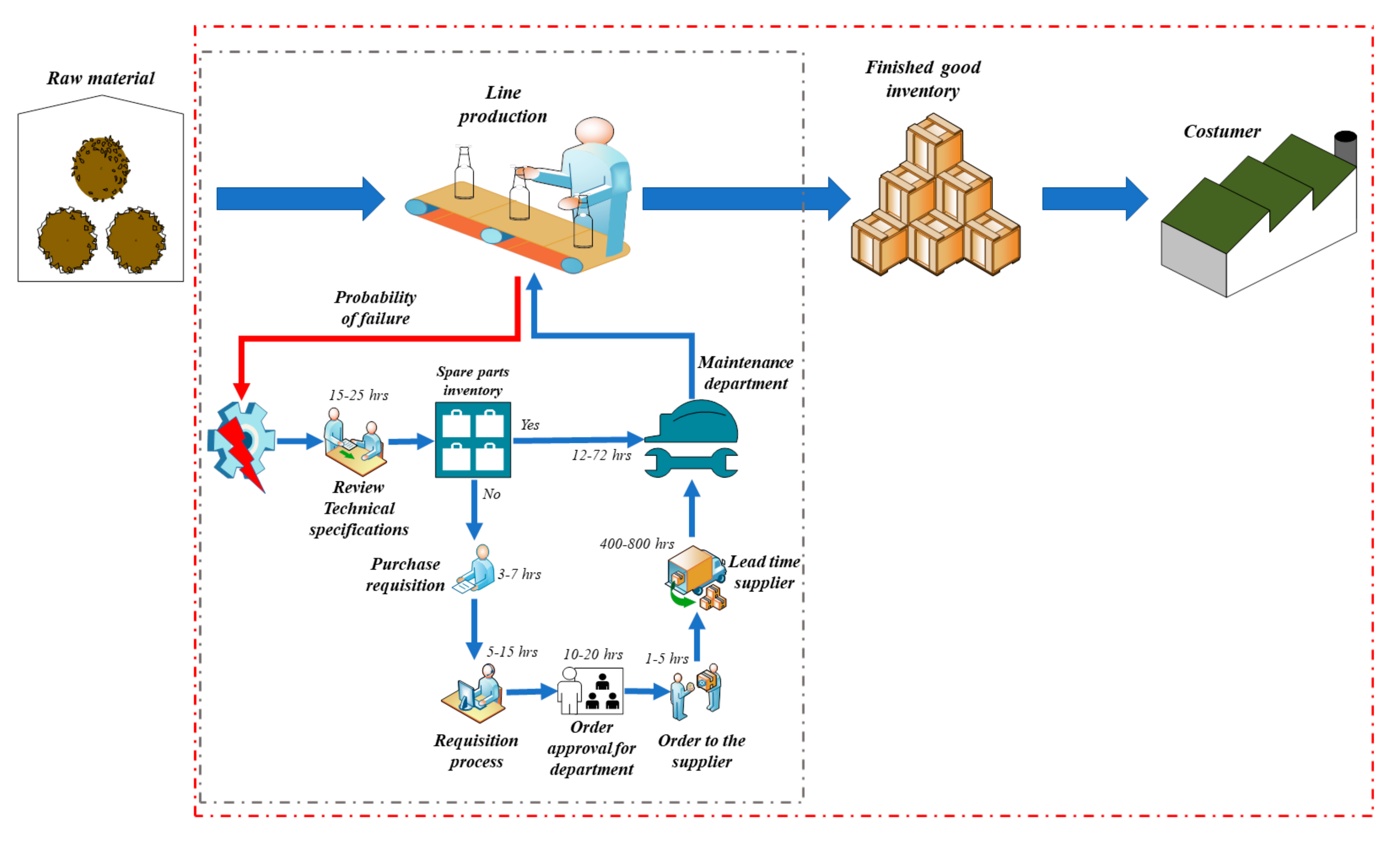
• The production department reviews the part’s technical specifications to submit a procurement request form. Then, the corresponding authorities at BPE analyze the information to set a price range for the part to be purchased. However, BPE’s authorities might return the purchase request form to the petitioners and demand a clearer form if the information on it seems confusing or incomplete.
• Once the purchase request is approved, the procurement department asks at least two suppliers for a proposal. All proposals must be thoroughly detailed, thus including information such as part price, lead time, purchase policies, and charged taxes, among others. The procurement department analyzes the proposals and then selects the most convenient one. This process is known as proposal solicitation.
• The production department is asked to approve the potential purchase order, purchase policies are again reviewed, and finally, the procurement department places a purchase order with the selected supplier, which in turn confirms the time when the spare part will be delivered.
• Following the delivery, BPE’s material inspectors examine the incoming material and review the purchase invoice. If everything is correct, the inspectors’ hand in the part to the production department. Then, the procurement department sends a payment confirmation form to the supplier, setting a payment date and time. Next, the recently purchased material is stocked as spare part inventory. If there is a problem with the order and/or the invoice, BPE’s material inspectors do not accept the received part and inform the procurement department of the issue. In turn, BPE’s procurement department negotiates with the supplier.

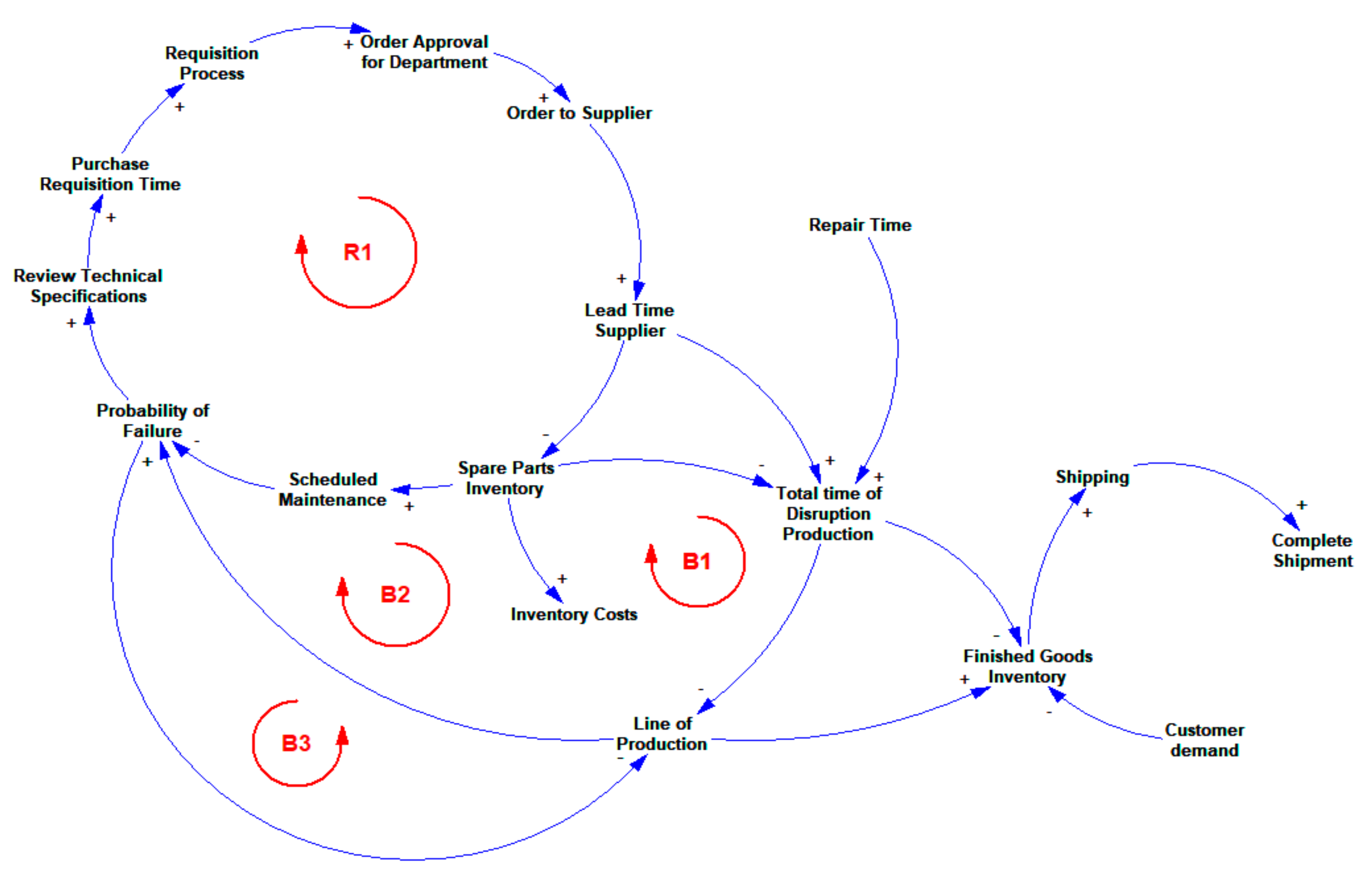
We used the aforementioned steps of BPE’s spare part procurement process to develop a causal diagram and identify the relationships among the different actors in the process.

3.1. Causal Diagram

Causal diagrams are graphical tools that help represent system behavior and identify interactions between system variables. In causal diagrams, variables are connected to each other through arrows indicating cause-effect relationships (A → B), which can be either positive or negative. In positive relationships, the values of the two variables (i.e., cause and effect) increase or decrease together; that is, an increase in the cause produces an increase in the effect, or a decrease in the cause leads to a decrease in the effect. On the other hand, in negative relationships, an increase in the cause produces a decrease in the effect, or a decrease in the cause leads to an increase in the effect. In causal diagrams, either reinforcing loops or balancing loops, are generated when an effect impacts on a cause. Balancing loops attempt to eliminate an effect, whereas reinforcing loops destabilize the system because of their snowballing effect [39,40].

Figure 2 depicts the causal diagram of a typical industrial spare part procurement process. As can be observed, the diagram shows critical times and key variables in the process. Some of these variables include technical specifications review, purchase requisition time, requisition process, order approval, order to supplier, supplier lead time, and spare part inventory. Additionally, the diagram indicates that spare part shortages both influece production disruptions and affect finished goods inventory. The feedback loops of this system are described as follows:

Loop R1. Variable Probability of Failure refers to the failure of any machine part in the production line, which triggers the activation of a spare part procurement process. This process involves different stages: technical specifications review, purchase requisition time, requisition process, order approval, order to supplier, and supplier lead time. Also, the procurement process is extensive and causes spare parts to arrive late in inventory, thus increasing the value of variable Scheduled Maintenance.

Loops B1 and B2. If variable Total Time of Production Disruption increases as a result of factors involved in the process, variable Production Rate decreases. However, when Production Rate increases, parts in machines wear out more rapidly, thus increasing Probability of Failure and causing production disruptions.

Loop B3. If Production Rate increases, Probability of Failure also increases. Conversely, if Production Rate decreases, Probability of Failure also decreases. Additionally, if Probability of Failure increases, Production Rate decreases.

In the following section, we discuss the equations used to develop the simulation model, which is based on the causal diagram depicted in Figure 2.

3.2. Equations

The equations take into account historical data from BPE on the following aspects: the production process, finished goods inventory management, spare part inventory management, records of disruptions caused by machine part failures, and procurement time of spare parts.

3.2.1. Probability of Failure

At BPE, records of disruption events derived from machine failures differ across production lines. Overall, we found that a same production line can endure one to four disruption events yearly. Hence, to represent a disruption event per year we defined Equation (1) as follows:

PULSE (1, RANDOM (0, 8760)).

(1)

The PULSE command in STELLA^® has the following format: PULSE [VOLUME, FIRST PULSE, INTERVAL]. We represented the VOLUME parameter with 1, since we only needed a value higher than 0 to represent a mechanical failure. As for the FIRST PULSE parameter, it had to indicate the time for the failure to occur. For this failure to occur randomly, we used the RANDOM command (RANDOM[MIN, MAX, SEED]) with 1 as the minimum value and 8760 (i.e., number of hours in a year) as the maximum value. We did not use SEED, since we needed the failures to be totally random. The INTERVAL parameter was not used either. This method allowed us to analyze only random mechanical failures; that is, we did not take into account scheduled maintenance sessions, which also cause production stoppages.

3.2.2. Raw Material Inventory (RMI)

The glass bottle manufacturing process relies on different types of raw materials, including silica sand, feldspars, and recycled glass, to name but a few. To represent BPE’s raw material consumption rate, we propose Equation (2) as follows:

$$RM{I}_t=RM{I}_{t=0}+{{\displaystyle \int }}_0^t\left(O{S}_{RM}-LP\right)dt,$$

(2)

where OS_RM stands for raw material orders delivered by suppliers, and LP refers to raw material consumption in the production line.

3.2.3. Finished Goods Inventory (FGI)

Glass bottles manufactured in the company are stocked as finished goods inventory to be delivered to customers. The equation used to calculate BPE’s finished good inventory is formulated below:

$$FG{I}_t=FG{I}_{t=0}+{{\displaystyle \int }}_0^t\left(LP-SD\right)dt,$$

(3)

where SD refers to scheduled deliveries to customers.

3.2.4. Spare Parts Inventory (SPI)

BPE’s spare part inventory can be calculated through Equation (4).

$$SP{I}_t=SP{I}_{t=0}+{{\displaystyle \int }}_0^t\left(ASP-SPC\right)dt,$$

(4)

where ASP stands for the arrival of spare parts in the company, and SPC refers to spare part consumption, due to either machinery maintenance or failures in the production lines.

3.2.5. Total Disruption Time (TDT)

When a given machine part fails or wears out, it must be replaced, thus activating BPE’s spare part procurement process. Each stage of this process entails a series of tasks, each of which take specific time to be accomplished. Consequently, the affected production line is stopped until the damaged part is successfully replaced in the machine. Unfortunately, production disruptions can severely affect downstream activities. To calculate total disruption time, we propose Equation (5):

$$TDT=\sum TSR+PRD+PR+OAD+O{S}_{SP}+LT+RT,$$

(5)

where TSR refers to the review of the part’s technical specifications, performed by material inspectors. If the spare part needed is on-site, the production line will be stopped only during the time it takes operators to replace the old part with the new part. On the other hand, if the spare part must be purchased, its technical specifications must be reported to the procurement department (PRD) by filling out a purchase request form. Also, in Equation (5), PR stands for the proposal request and comprises from the moment the company asks proposals to suppliers to the moment the department requesting the spare part (OAD) approves a proposal. Once the proposal is approved, the purchase order is sent to the supplier (OSSP), and lead time (LT) begins. Once the spare part arrives at BPE, repair time (RT) initiates. Finally, TDT is the sum of all the aforementioned time intervals.

3.2.6. Line of Production (LP)

To simulate production rate in BPE’s production line, we used a normal distribution with an average of 3650 glass bottles and a standard deviation of 50 glass bottles (see Equation (6)).

LP = N (3650, 50)

(6)

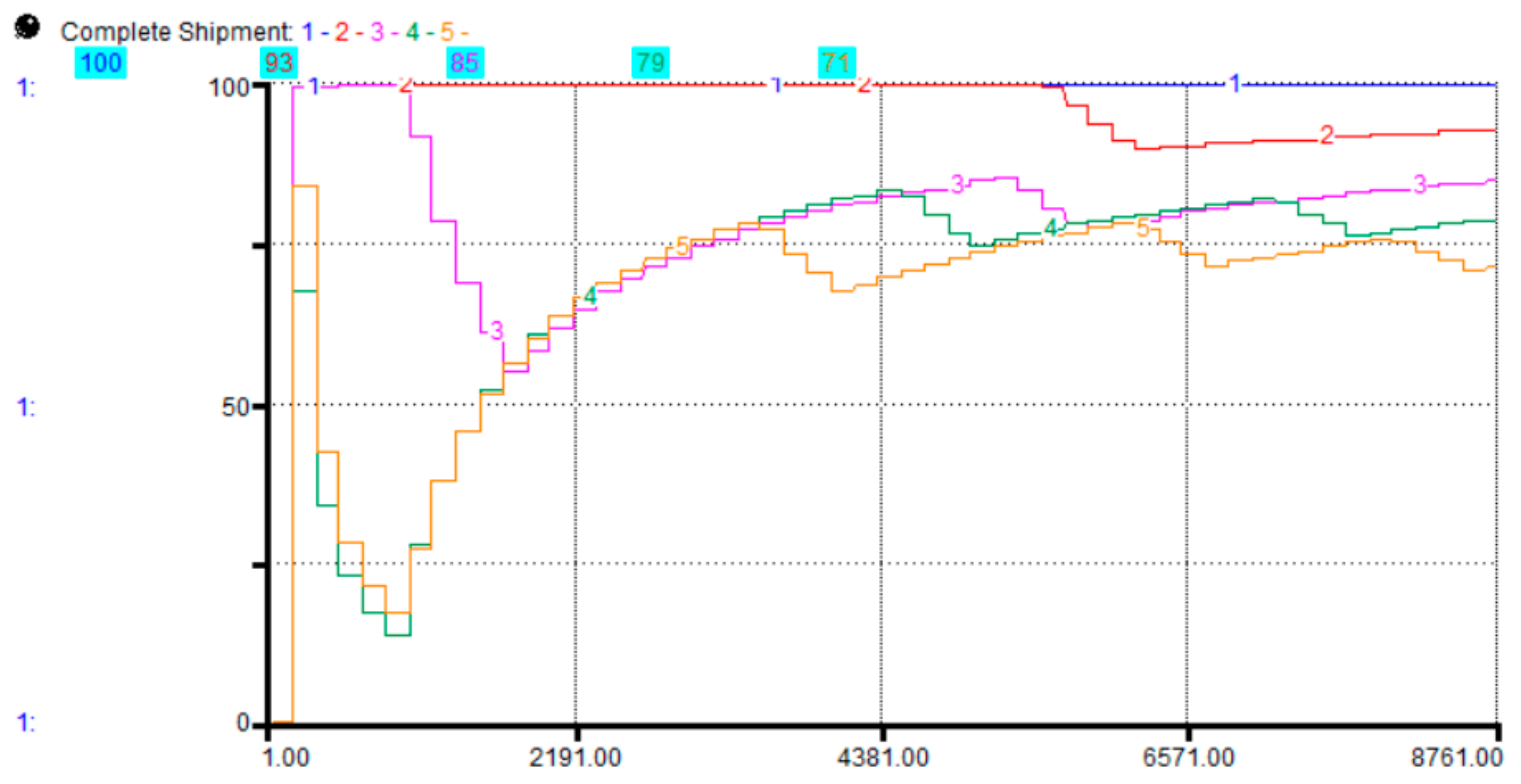
3.2.7. Complete Shipment (CS)

We used Equation (7) as an indicator of complete deliveries shipped to customers:

CS = NODF/TOP,

(7)

where NODF indicates the total number of complete deliveries, and TOP refers to the total orders delivered within a period of time.

3.2.8. Initial Parameters

We used STELLA^® software to develop the simulation model. The length of the time horizon was 8760 h (i.e., a year) with a Delta Time (DT) of one hour to generate results each hour. As for the model parameters,

Table 1. Initial simulation parameters.

Variables	Values without Spare Part	Values with Spare Part	Units
Line of production	N (3650, 50)	N (3650, 50)	Pieces
Spare Parts Inventory	0	≥1	Pieces
Review Technical Specification	15–25	15–25	Hours
Purchase Requisition Time	3–7	0	Hours
Requisition Process	5–15	0	Hours
Order Approval for Department	10–20	0	Hours
Order to Supplier	1–5	0	Hours
Supplier Lead Time	400–800	0	Hours
Repair Time	12–72	12–72	Hours
Raw Material Inventory	300,000	300,000	Kg
Finished Goods Inventory	100,000	100,000	Bottles
Weekly Customer orders	600,000	600,000	Bottles

lists BPE’s average times for part acquisition, production rate, initial raw material inventory, finished goods inventory, and weekly customer orders.

4. Results and Discussion

This section discusses the results obtained from the simulation model.

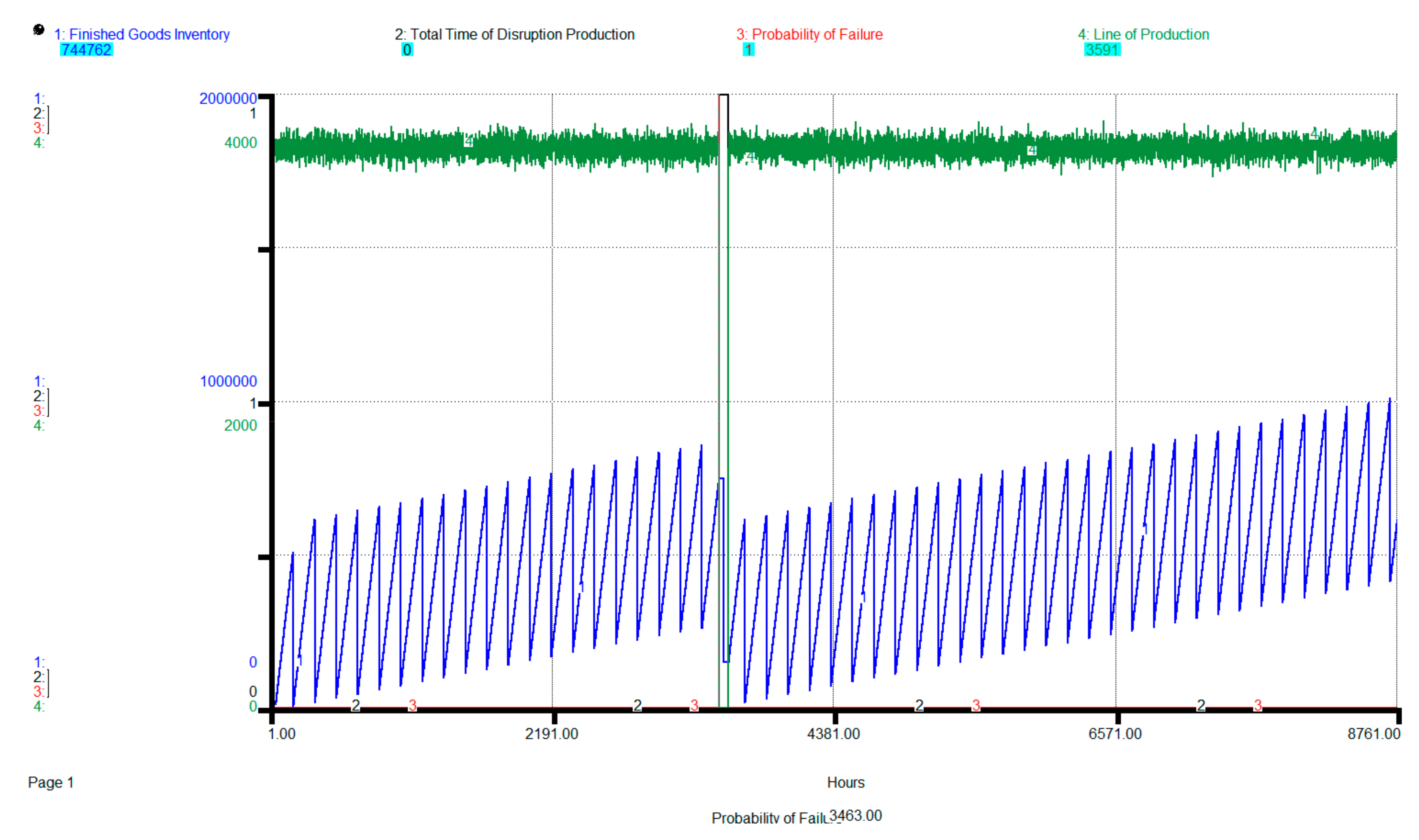
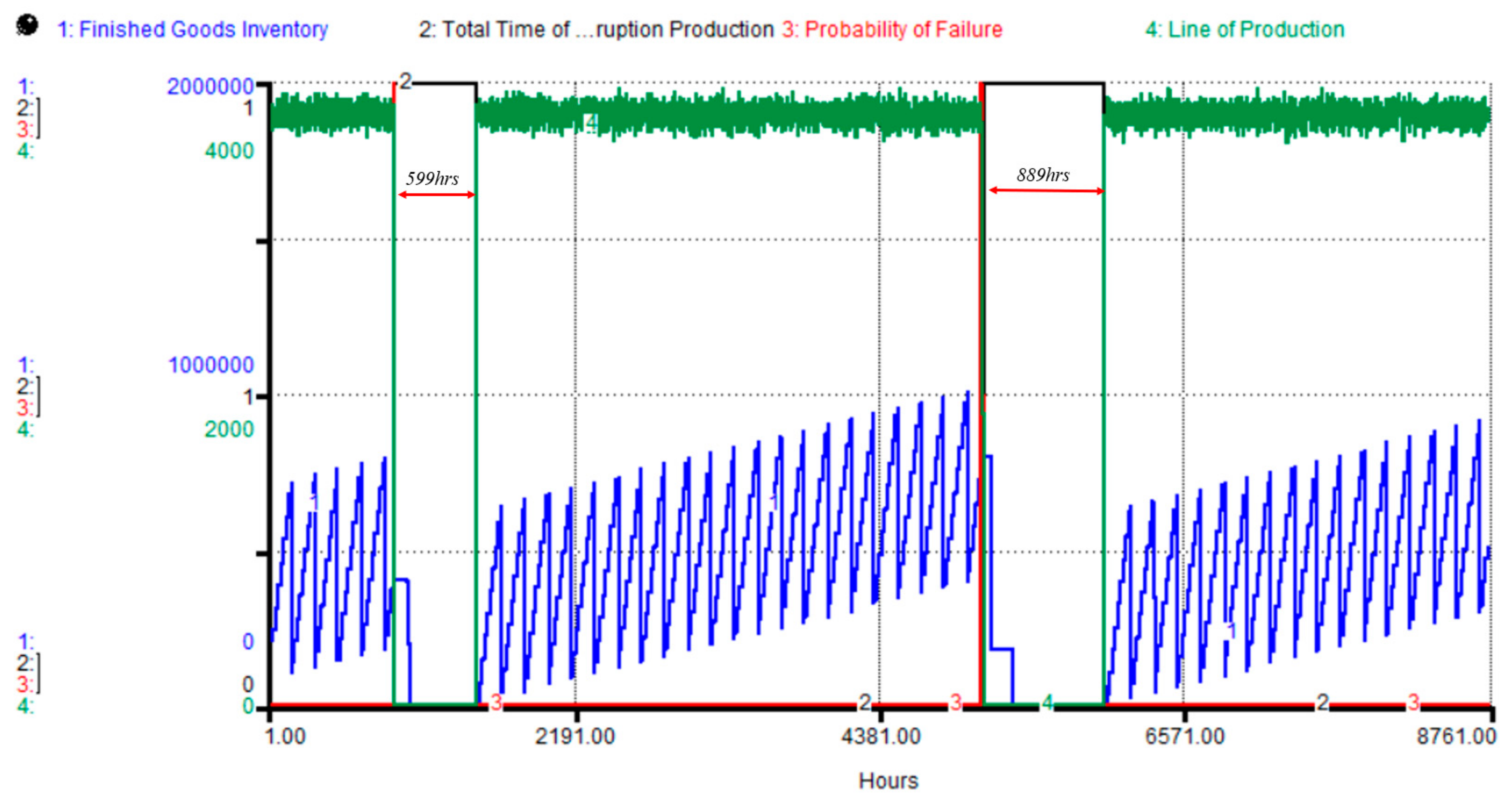
4.1. Initial Simulation

We ran the simulation model for the first time using the values listed in Table 1. According to the results, depicted in Figure 3, the mechanical failure occurs in hour 3463. Then, the process of replacing the damaged part and repairing the machine begins. If the spare part needed is in stock, the production disruption lasts 68 h, i.e., 20 h for technical inspection and machine dismantling and 48 h for part replacement. Additionally, during the disruptive event, the level of finished goods inventory decreases, yet it does not compromise scheduled deliveries, since the disruption lasts only for a short time.

Conversely, if the spare part needed to fix the machine is not in stock (Figure 4), the spare part procurement process begins, comprising the tasks and times listed in Table 1. In this case, the production disruption lasts 716 h. The level of finished goods inventory drops to 0, but then, it gradually stabilizes again.

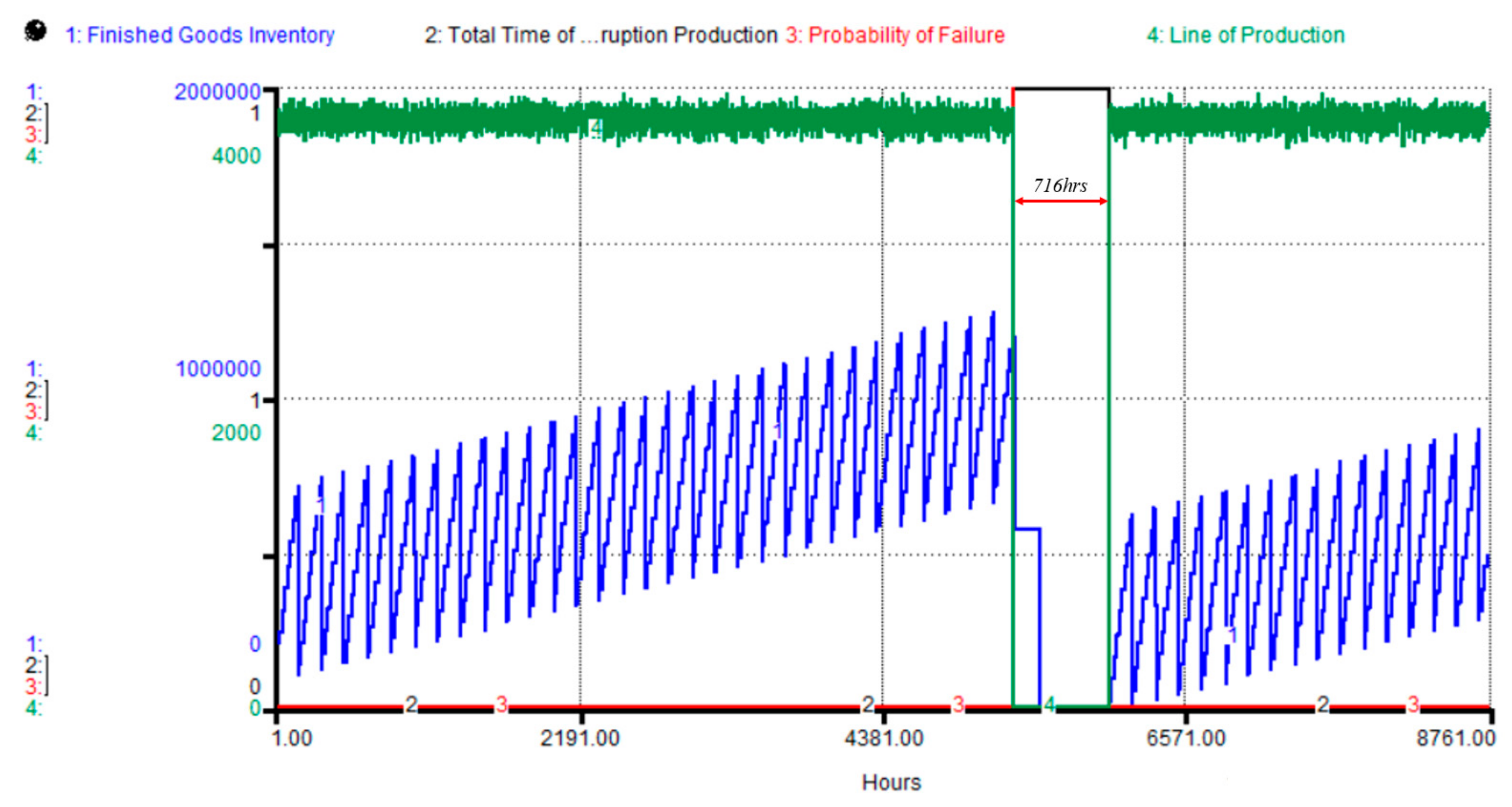
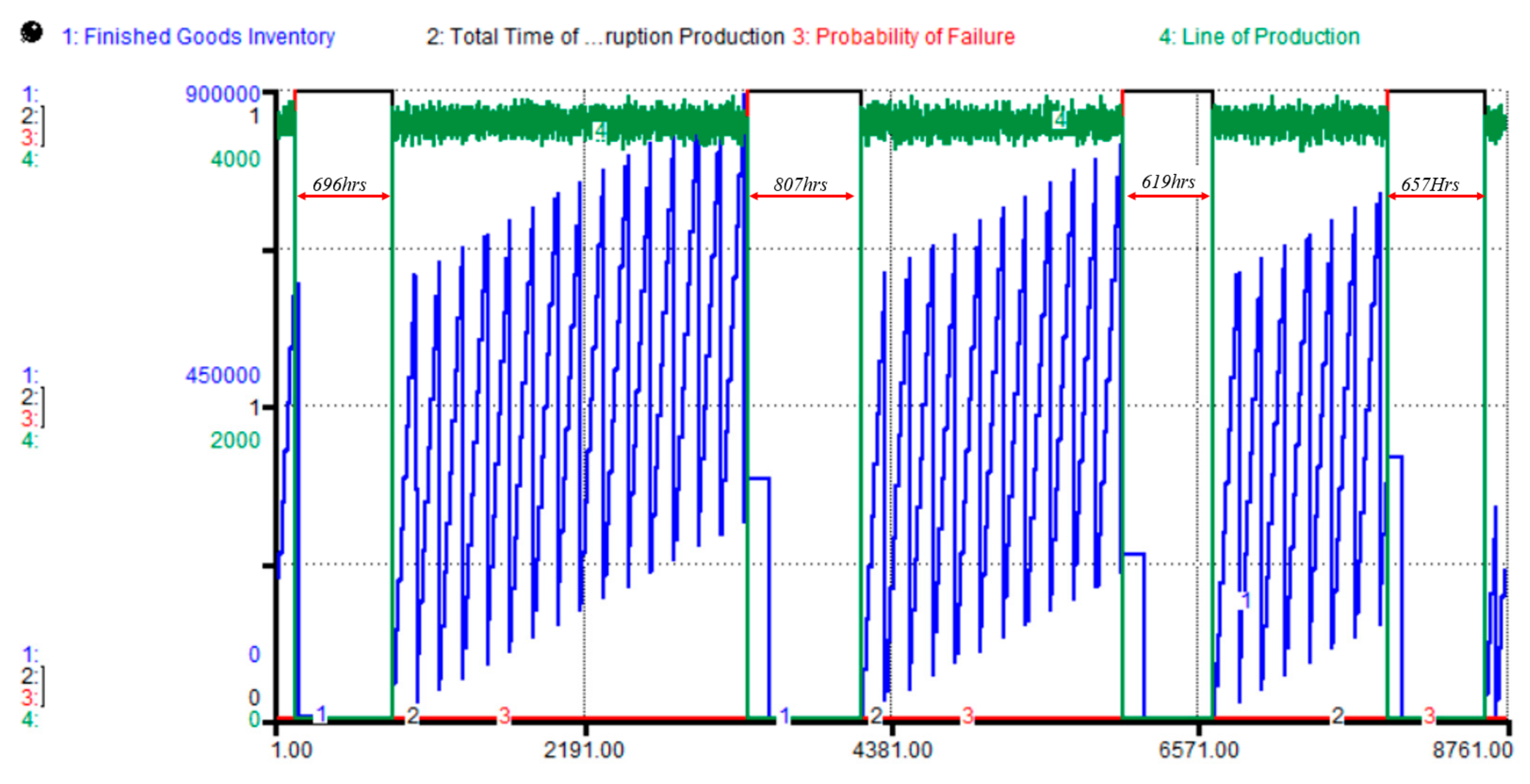
4.2. Multiple-Failure Scenario

If customer orders increase from 600,000 to 620,000 glass bottles, production must also increase from 3650 to 3800 bottles per hour in order to successfully meet the demand. However, as depicted in the causal diagram, higher production rates can lead to greater probability of machine failure. Figure 5 depicts a simulation scenario in which two machine failures occur in the production line, and the machine’s spare parts are not in stock. The first failure occurs in hour 871 and lasts for 599 h. The second failure occurs in hour 5106 and lasts for 889 h. The two disruptive events have a direct impact on both the level of finished goods inventory and the rate of orders fully shipped to customers.

We ran the model several times to determine its robustness and find out what could happen if three disruptive events occurred in BPE’s production line within a year. As Figure 6 illustrates, the first disruption occurred in hour 78 and lasted for 754 h. The second disruptive event occurred in hour 4332 and lasted for 719 h. Finally, the third disruptive event happened in hour 7059 and lasted for 600 h.

Since BPE claims to have endured a maximum of four disruptive events in a year, we ran the model several times until such scenario arose. As can be observed from Figure 7, the first disruption occurred in hour 97 and lasted for 696 h. The second disruptive event occurred in hour 3346 and lasted for 807 h. The third disruptive event occurred in hour 6015 and lasted for 619 h. Finally, the fourth disruptive event appeared in hour 7910 and lasted for 657 h. As can be observed from the graphs, each of the four disruptions occurred at a different time interval and had a different duration.

Figure 8 compares the five aforementioned scenarios. During a disruptive event derived from a damaged or worn out part, BPE can meet 100% of its demand if the spare part needed to fix the machine is on-site. Nevertheless, if the spare part is out of stock, only 93% of customer orders can be fulfilled. If two, three, or four disruptive events occur in a year, and if the spare parts needed to fix the machines are out of stock, BPE can only fulfill 85%, 79%, and 71% of customer orders, respectively. In conclusion, two or more scenarios compromise BPE’s 98%–100% complete delivery.

As depicted in Figure 1, BPE’s spare part procurement protocol comprises seven processes, whose duration may vary from one another.

Table 2. Impact of process duration on Complete Shipment.

			Repair Time (12–72 h)
			Supplier Lead Time (400–800 h)
			Order to Supplier (1–5 h)
			Order Approval for Department (10–20 h)
			Requisition Process (5–15 h)
			Purchase Requisition Time (3–7 h)
			Review Technical Specification (15–25 h)
			Run (percentages)
Disruption	Min	Max	1	2	3	4	5	6	7	8	9	10
1	90.98	96.68	92.62	94.27	94.53	92.31	93.98	96.05	91.85	92.96	92.15	94.99
2	79.77	91.35	84.54	84.83	87.32	86.45	88.05	85.5	90.08	83.59	85.49	83.58
3	69.25	86.69	77.47	74.59	75.17	75.87	77.01	77.49	84.52	75.68	74.92	78.04
4	60.35	81.78	68.98	80.05	66.97	70.71	72.24	67.08	67.86	77.21	72.64	66.42

shows how the duration of each process can affect the Complete Shipment indicator at BPE. For instance, with a Finished Product Inventory of 100,000 glass bottles and one mechanical failure, the indicator Complete Shipment can occur in an interval with a minimum value of 90.98% and a maximum value of 96.98%. Conversely, if two mechanical failures occur, Complete Shipment has an interval of 79.77% to 91.35%. If three mechanical failures happen, BPE is able to meet complete shipment in an interval of 69.25% to 86.69%. Finally, in the light of four mechanical disruptions, Complete Shipment is reached only in 60.35% to 81.78%. To evaluate and validate the maximum and minimum percentages discussed below, we ran 10 scenarios per failure, which also are shown in Table 2, and the values that occur are between the minimum and maximum values found.

4.3. Sensitivity Analysis

Order shipping is a key firm performance indicator that may be easily compromised when companies cannot stock all the spare parts of each production machine. In this section, we propose a sensitivity analysis to identify those scenarios in which high order shipping rates can be achieved under a production rate of 3800 glass bottles per hour and weekly orders of 600,000 bottles. We performed a sensitivity analysis to determine the minimum level of finished product inventory that BPE needs to ensure in order to comply with its Complete Shipment policy in the light of one, two, three, or even four mechanical failures.

Table 3. Results for 200 scenarios.

		Repair Time (12–72 h)
		Supplier Lead Time (400–800 h)
		Order to Supplier (1–5 h)
		Order Approval for Department (10–20 h)
		Requisition Process (5–15 h)
		Purchase Requisition Time (3–7 h)
		Review Technical Specification (15–25 h)
		Run (percentages)
FGI	Disruption	1	2	3	4	5	6	7	8	9	10
200,000	1	93.13	92.84	92.48	93.44	95.52	92.03	94.05	96.02	95.35	93.54
	2	81.19	89.65	84.32	83.28	85.34	90.05	91.5	82.08	87.2	81.25
	3	83.95	72.68	71.23	70.54	82.28	85.24	78.32	86.2	73.21	75.22
	4	77.45	65.23	68.45	80.22	65.23	78.52	81.24	70.29	79.32	75.41
400,000	1	92.23	93.04	95.23	97.02	92.17	94.25	95.37	96.21	93.24	92.52
	2	84.87	85.23	81.28	86.23	87.54	88.22	89.46	90.21	81.18	91.02
	3	71.09	75.23	74.58	72.25	77.85	76.59	85.23	75.89	77.24	80.02
	4	81.54	81.73	68.52	63.64	74.8	69.02	79.63	79.48	81.21	77.35
600,000	1	93.85	92.68	94.02	92.95	96.14	93.86	96.96	92.61	96.01	95.61
	2	84.29	86.11	92.26	95.15	83.47	96.11	89.36	97.81	96.81	87.67
	3	82.24	86.69	91.46	86.28	92.65	88.93	85.39	88.45	90.56	92.65
	4	73.19	82.58	71.53	72.4	71.5	87.7	74.84	72.56	71.76	85.37
800,000	1	94.60	98.66	95.84	95.06	96.35	96.1	97.71	97.88	95.34	94.12
	2	84.99	82.92	91.45	86.7	82.48	83.11	90.57	84.49	86.99	88.9
	3	75.00	76.81	86.18	72.93	77.34	76.39	80.45	78.35	74.53	85.92
	4	67.23	74.25	81.57	83.75	75.18	68.76	83.64	67.28	83.05	81.33
1,000,000	1	94.61	96.74	95.97	97.94	99.14	99.79	98.53	94.86	95.62	98.73
	2	85.28	86.01	83.82	88.49	88.59	87.67	87.77	83.82	85.93	91.44
	3	75.53	87.21	79.93	87.74	79.76	80.79	76.03	79.83	82.97	75.07
	4	68.64	75.5	77.68	73.61	76.33	70.23	75.26	69.3	83.59	76.84

summarizes the results of the 200 scenarios. The analysis takes into account different levels of finished product inventory, the seven processes comprised in BPE’s spare pare procurement protocol, and the occurrence of one to four mechanical failures. According to the analysis results, BPE can comply with its complete shipment policy in five scenarios, where, the minimum level of Finished Goods Inventory is 800,000 glass bottles (one possible scenario), although the chances for BPE to comply with its complete shipment policy increase when the company has a stock of 1,000,000 glass bottles (four possible scenarios). However, with two or more mechanical failures in a year, BPE would not be able to ensure such level of Finished Goods Inventory.

5. Conclusions and Future Work

The main contribution in this research is that it assesses the impact of machine part failures on a production line in a glass manufacturing company, for which a model developed using the System Dynamics methodology is proposed. The model allows systematic analysis of the impact that a disruption generates in the production process over other key logistics processes of the company, such as distribution. After running a simulation model, it was found that if the spare part needed to fix the mechanical failure is on-site, the production line will stop only during the time it takes the company to replace the old part with the new part. Nevertheless, if the spare part is not in stock, the spare part procurement process begins, which might extend the duration of the disruptive event for weeks, affecting delivery dates promised. In the end, the simulation model revealed that mechanical failures have a direct impact on order shipping rates and that affects the company’s reputation and corporate image. Three scenarios were proposed to assess the performance of our simulation model, which can be replicated in other companies.

These scenarios allowed managers to understand the importance of spare part inventory management in the light of unexpected disruptive events. Finally, a sensitivity analysis was run on 200 scenarios to identify those combinations of variables that can help the company comply with its 98–100% order shipping policy. As remarks for future work, we suggest both performing an analysis of costs derived from production disruptions and conducting a sensitivity analysis with other variables, such as increased production, multiple suppliers, and probability of failure, among others. Likewise, the authors propose to evaluate other strategies that improve the company’s performance in complete orders delivered to customers, such as using other company production lines or adjusting the production schedule, aspects that were not considered in this model.

References

1. Wang, Y.; Huang, M.; Chen, J. System Dynamics Modeling of backup purchasing strategies under supply disruptions risks. Int. J. Serv. Sci. Technol. 2014, 7, 287–296. [Google Scholar] [CrossRef]
2. Charles, A.; Lauras, M.; Van Wassenhove, L. A model to define and asses the agility of supply chains: Building on hummanitarian experience. Int. J. Phys. Distrib. Logist. Manag. 2010, 40, 722–741. [Google Scholar] [CrossRef] [Green Version]
3. Kiperska-Moron, D.; Swierczek, A. The agile capabilities of polish companies in the supply chain: An empirical study. Int. J. Prod. Econ. 2009, 118, 217–224. [Google Scholar] [CrossRef]
4. Hu, X.; Gurnani, H.; Wang, L. Managing risk of supply disruptions: Incentives for capacity restoration. Prod. Oper. Manag. 2013, 189, 137–150. [Google Scholar] [CrossRef]
5. Cárdenas-Barrón, L.E.; Akbar Shaikh, A.; Tiwari, S.; Treviño-Garza, G. An EOQ inventory model with nonlinear stock dependent holding cost, nonlinear stock dependent demand and trade credit. Comput. Ind. Eng. 2018, in press. [Google Scholar]
6. Mehdizadeh, M. Integrating ABC analysis and rough set theory to control the inventories of distributor in the supply chain of auto spare parts. Comput. Ind. Eng. 2019, in press. [Google Scholar] [CrossRef]
7. Alakan, A.; Nishanth, D.; Nagaraju, D.; Narayanan, S.; Devendiran, S. On the Optimality of Inventory and Shipment Decisions in a Joint Three Echelon Inventory Model with Finite Production Rate under Stock Dependent Demand. Procedia Manuf. 2019, 30, 490–497. [Google Scholar] [CrossRef]
8. Thinakaran, N.; Jayaprakas, J.; Elanchezhian, C. Survey on Inventory Model of EOQ & EPQ with Partial Backorder Problems. Mater. Today Proc. 2019, 16, 629–635. [Google Scholar]
9. Tank, L.; Jing, K.; He, J.; Stanley, H. Complex interdependent supply chain networks: Cascading failure and robustnees. Phys. A Stat. Mech. Appl. 2016, 443, 58–69. [Google Scholar] [CrossRef]
10. Dominguez, R.; Cannella, S.; Framinan, J. On returns and network configuration in supply chain dynamics. Transp. Res. Part E Logist. Transp. Rev. 2014, 73, 152–167. [Google Scholar] [CrossRef]
11. Zhu, S.; Jaarsveld, W.; Dekker, R. Spare Parts Inventory Control based on Maintenance Planning. Reliab. Eng. Syst. Saf. 2019, in press. [Google Scholar] [CrossRef]
12. Rahimi-Ghahroodi, S.; Hanbali, A.A.; Vliegen, I.; Cohen, M. Joint optimization of spare parts inventory and service engineers staffing with full backlogging. Int. J. Prod. Econ. 2019, 212, 39–50. [Google Scholar] [CrossRef]
13. Basten, R.J.; Ryan, J.K. The value of maintenance delay flexibility for improved spare parts inventory management. Eur. J. Oper. Res. 2019, 278, 646–657. [Google Scholar] [CrossRef]
14. Turrini, L.; Meissner, J. Spare parts inventory management: New evidence from distribution fitting. Eur. J. Oper. Res. 2019, 272, 118–130. [Google Scholar] [CrossRef]
15. Umeda, S.; Lee, Y.T. Design specifications of a generic supply chain simulator. In Proceedings of the Winter Simulation Conference, Washington, DC, USA, 5–8 December 2004. [Google Scholar]
16. Forrester, J. System dynamics—A personal view of the first fyfty years. Syst. Dyn. Rev. 2007, 23, 345–358. [Google Scholar] [CrossRef]
17. Matsuo, H. Implications of the Tohoku earthquake for Toyota’s coordination mechanism: Supply chain disruption of automotive semiconductors. Int. J. Prod. Econ. 2015, 161, 217–227. [Google Scholar] [CrossRef]
18. Siswanto, N.; Kurniawati, U.; Latiffianti, E.; Rusdiansyah, A.; Sarker, R. A Simulation study of sea transport based fertilizer product considering disruptive supply and congestion problems. Asian J. Shipp. Logisti. 2018, 34, 269–278. [Google Scholar] [CrossRef]
19. Adediran, T.V.; Al-Bazi, A.; Dos Santos, L.E. Agent-based modelling and heuristic approach for solving complex OEM flow-shop productions under customer disruptions. Comput. Ind. Eng. 2019, 133, 29–41. [Google Scholar] [CrossRef]
20. Ivanov, D. Disruption tails and revival policies: A simulation analysis of supply chain design and production-ordering systems in the recovery and post-disruption periods. Comput. Ind. Eng. 2019, 127, 558–570. [Google Scholar] [CrossRef]
21. Li, S.; He, Y.; Chen, L. Dynamic strategies for supply disruptions in production-inventory systems. Int. J. Prod. Econ. 2017, 194, 88–101. [Google Scholar] [CrossRef]
22. Beccue, P.C.; Huntington, H.G.; Leiby, P.N.; Vincent, K.R. An updated assessment of oil market disruption risks. Energy Policy 2018, 115, 456–469. [Google Scholar] [CrossRef]
23. Basten, R.; Houtum, G. System-oriented inventory models for spare parts. Surv. Oper. Res. Manag. Sci. 2014, 19, 34–55. [Google Scholar] [CrossRef] [Green Version]
24. Ghorbel, N.; Addouche, S.A.; Mhamed, A.E. Forward management of spare parts stock shortages via causal reasoning using reinforcement learning. IFAC-PapersOnLine 2015, 48, 1061–1066. [Google Scholar] [CrossRef]
25. Sarker, R.; Haque, A. Optimization of maintenance and spare provisioning policy using simulation. Appl. Math. Model. 2000, 24, 751–760. [Google Scholar] [CrossRef]
26. Hong, Y.S.; Huh, W.T.; Kang, C. Sourcing assemble-to-order inventories under supplier risk uncertainty. Omega 2017, 66, 1–14. [Google Scholar] [CrossRef]
27. Hishamuddin, H.; Sarker, R.; Essam, D. A disruption recovery model for a single stage production-inventory system. Eur. J. Oper. Res. 2012, 222, 464–473. [Google Scholar] [CrossRef]
28. Kader, B.; Sofiene, D.; Nidhal, R.; Walid, E. Joint optimization of preventive maintenance and spare parts inventory for an optimal production plan with consideration of CO2 emission. Reliab. Eng. Syst. Saf. 2016, 149, 172–186. [Google Scholar]
29. Tomlin, B.T. On the Value of a Threat Advisory System for Managing Supply Chain Disruptions. Ph.D. Thesis, University of North Carolina at Chapel Hill, Chapel Hill, NC, USA, 2009. [Google Scholar]
30. Tomlin, B.T.; Snyder, L.V. On the value of mix flexibility and dual sourcing in unreliable newsvendor networks. Manuf. Serv. Oper. Manag. 2005, 7, 37–57. [Google Scholar] [CrossRef]
31. Kumar, D.; Kumar, D. Modelling rural healthcare supply chain in India using system dynamics. Procedia Eng. 2014, 97, 2204–2212. [Google Scholar] [CrossRef] [Green Version]
32. Gröne, S.; Förster, S.; Hiete, M. Long-term impact of environmental regulations and eco-conscious customers in the chemical industry: A system dynamics approach to analyze the effect of multiple disruptions. J. Clean. Prod. 2019, 227, 825–834. [Google Scholar] [CrossRef]
33. Song, M.; Cui, X.; Wang, S. Simulation of land green supply chain based on system dynamics and policy optimization. Int. J. Prod. Econ. 2018, in press. [Google Scholar] [CrossRef]
34. Mota-López, D.R.; Sánchez-Ramírez, C.; Alor-Hernández, G.; García-Alcaraz, J.L.; Rodríguez-Pérez, S.I. Evaluation of the impact of water supply disruptions in bioethanol production. Comput. Ind. Eng. 2019, 127, 1068–1088. [Google Scholar] [CrossRef]
35. MacKenziea, A.; Miller, J.; Hill, R.R.; Chambal, S.P. Application of agent based modelling to aircraft maintenance manning and sortie generation. Simul. Model. Pract. Theory 2012, 20, 89–98. [Google Scholar] [CrossRef]
36. Kim, B.; Kim, K. Estimating the effect of module failures on the gross generation of a photovoltaic system using agent-based modeling. Renew. Sustain. Energy Rev. 2018, 91, 1019–1024. [Google Scholar] [CrossRef]
37. Liu, Y.; Wang, T.; Zhang, H.; Cheutet, V.; Shen, G. The design and simulation of an autonomous system for aircraft maintenance scheduling. Comput. Ind. Eng. 2019, 137, 106041. [Google Scholar] [CrossRef] [Green Version]
38. Alrabghi, A.; Tiwari, A. A novel approach for modelling complex maintenance systems using discrete event simulation. Reliab. Eng. Syst. Saf. 2016, 154, 160–170. [Google Scholar] [CrossRef] [Green Version]
39. Lewis, B.M.; Erera, A.L.; Nowak, M.A.; White, C.C. Managing Inventory in Global Supply Chains Facing Port-of-Entry Disruption Risks. Transp. Sci. 2013, 45, 89–109. [Google Scholar] [CrossRef]
40. Tomlin, B. On the value of mitigation and contingency strategies for managing supply chain disruptions risk. Manag. Sci. 2006, 52, 639–657. [Google Scholar] [CrossRef] [Green Version]
Figure 1. Model analyzed in a BPE (Bottle Processing Enterprise) company.
Applsci 10 00208 g001
Figure 2. Causal loop diagram of the system for supplying special parts.
Applsci 10 00208 g002
Figure 3. Time of disruption in production line with spare parts in inventory.
Applsci 10 00208 g003
Figure 4. Time of disruption in line of production without spare parts in inventory.
Applsci 10 00208 g004
Figure 5. Disruption time in line of production with multiple failures.
Applsci 10 00208 g005
Figure 6. Disruption time in line of production with three failures.
Applsci 10 00208 g006
Figure 7. Disruption time in line of production with four failures.
Applsci 10 00208 g007
Figure 8. Complete Shipment in the five scenarios.
Applsci 10 00208 g008