Fault Detection in Multi-Core C&I Cable via Machine Learning Based Time-Frequency Domain Reflectometry ^†

Abstract

The integrity and functionality of the control and instrumentation (C&I) cable systems are essential when it comes to ensuring the reliability and safety of system operations, especially in vehicles or power plants. Whenever a fault occurs in a multi-core cable, it not only affects signals of the individual faulty line but inflicts the rest through crosstalk and noise interference. Thus, it is imperative that cable diagnostic technologies are eligible of detecting the fault and further differentiating the faulty line to prevent the original fault from jeopardizing the entire system operation. We propose here a diagnostic method which detects the presence and the location of a fault, and further differentiates the faulty line within the multi-core C&I cables using a machine learning algorithm based on the time-frequency domain reflectometry results. Neural networks and the hierarchy clustering algorithm are used for fault detection and the identification of the faulty line. The proposed clustering algorithm is verified via experiments with four possible fault scenarios using automotive wires and C&I cables for nuclear power plants. Hence, the proposed algorithm allows a fault in multi-core cables to be accurately detected and estimated when given the location and the reflection coefficient of a fault.

1. Introduction

In various industrial fields, control and instrumentation (C&I) cables assure the stability and reliability of system operations through controlling systems, transmitting signals, and monitoring networks. Likewise, in nuclear power plants (NPP), ensuring the integrity of electrical cables, which is highly relevant with the coolant system, safety injection system, and the containment spray system, is essential for plant operation [1]. The multi-core C&I cables in NPPs are generally installed to minimize both space and cost as well as prevent wiring labor in limited areas. Moreover, C&I cables are often installed in containment areas under the conditions of high temperature and high radiation, thus exposing their polymeric insulation materials to chemical/physical changes. Consequently, faults resulting from various external stresses inflict errors in the C&I signals, signal leakages, and interference noises in the multi-core cables, which pose serious threats to the operation of the NPP. Therefore, it is of paramount importance to accurately distinguish the faulty line among others and to instantaneously detect the fault upon its occurrence to prevent any accidents which may lead to severe health problems and economic losses.

Safety measures should also be established for multi-wires inside automotive electronics of vehicles. In automotive electronics, cables and connectors are usually installed near vibration motors and wheels. Thus, the wires subjected to vibration and heat damage are highly susceptible of causing failures during operation [2,3]. Wiring failures causing the detrimental situations of uncontrollable vehicles or sudden breakdowns endanger both the driver and the pedestrians, leading to secondary damages.

The reflectometry technique, a non-invasive electrical cable diagnosis method, possesses the capacity of detecting faults and assessing cable conditions [4]. When an impedance change is caused by a fault or degradation due to operations in a C&I cable, a propagated signal is reflected and transmitted at the local impedance discontinuity point depending on the reflection coefficient [5]. Reflectometry can be divided into two categories depending on its domain of analysis: the time domain reflectometry (TDR) and frequency domain reflectometry (FDR) [6,7]. Both methods are easy to implement and need not require high voltages. Unfortunately, the diagnostic results of both the TDR and FDR method are highly susceptible to electric noise and crosstalk [8,9]. Moreover, signal attenuation, distortion, and dispersion, which are all likely to occur in the measured reflected signal during signal propagation, diminish the accuracy and reliability of the diagnostic results. Conversely, the time-frequency domain reflectometry (TFDR) method simultaneously analyzes the reflected signal in both the time and frequency domains, which compensates for the drawbacks of the conventional methods [9]. Herein, the incident signal can be designed in the time and frequency domains according to the characteristics of the cable, and the impedance discontinuity points in the cable can be detected using the time-frequency distribution similarities between the incident signal and the reflected signal. Therefore, reflected signals are less likely to be affected by the cable propagation characteristics or external noises. However, existing reflectometry methods focus on diagnosing a single or pair core cable and is thereby unsuitable for multi-core cables or wired networks. When reflectometry is applied to a multi-core cable, the reflected signal generated at an actual fault point of a defective line is introduced to a normal line and can be measured due to crosstalk [10].

This paper presents a multi-core cable diagnosis method which detects faults and distinguishes faulty lines using the machine learning-based TFDR. First, the location and type of cable fault are detected using a regression-based artificial neural network (ANN) of the TFDR results [11,12]. Then, the data clustering is used to differentiate the faulty lines. Various existing clustering algorithms are selectively used based on crisp [13], fuzzy [14], and possibility methods [15,16]. The hierarchy clustering algorithm is an unsupervised machine learning algorithm which builds a hierarchy of clusters based on group similarities without any knowledge about the pre-defined groups [17,18]. The main advantage of the hierarchical clustering over partial clustering is that a hierarchy dendrogram can be drawn to find the appropriate number of clusters in a dataset.

This paper extends the contribution of [19] in terms of the theoretical algorithm of fault detection and differentiation. In [19], we investigated the faulty line detection in a multi-core cable by using K-means clustering-based TFDR. When a fault occurred, results showed that other normal lines were affected at similar points in the multi-core cable. However, only the identification of the faulty line within the multi-core cable had been considered in the study. Moreover, classifying the impedance discontinuity points from the TFDR results in the multi-core cable have not been considered in [19] which is important for applications to the multi-core cable diagnosis. On the other hand, the applicability of the proposed algorithm in this paper is verified through additional experiments using various types of multi-core cables. To achieve this goal, we extracted input features of the TFDR results and learned each machine learning algorithm for diagnostic purposes. The detection and clustering results obtained from the experimental fault scenarios reveal that clustering TFDR results can be used for fault locating faulty line identification among a pool of normal lines in a multi-core cable. The following sections describe the TFDR, ANNs, and clustering algorithms that are used to detect and analyze the fault in multi-core cables. In Section 3, we present cable fault scenarios and our experimental setup, and, in Section 4, we discuss the obtained experimental results. Finally, we conclude the paper in Section 5.

2. Theoretical Background

2.1. Time-Frequency Domain Reflectometry

The TFDR process consists of three steps: (1) First, we designed the optimal incident signal, which is applied to the cable, and (2) the reflected signal is then measured. (3) Then, we calculated the time-frequency cross-correlation (TFCC) between the reference signal and the reflected signal [9].

The TFDR uses a Gaussian envelope with a linear chirp signal as a reference signal, which can be expressed as follows [9]:

$$s\left(t\right)=exp\left(\frac{-{(t-t_0)}^2}{2{\tau }_0^2}\right)exp\left(j\frac{1}{2}{\dot{\omega }}_0{(t-t_0)}^2+j{\omega }_0(t-t_0)\right)$$

(1)

where ${\tau }_0$ is the effective time duration, $t_0$ is the center time, ${\omega }_0$ is the center frequency of the chirp signal, and ${\dot{\omega }}_0$ is the frequency increment by time.

The reflected signals are attenuated and distorted over the entire frequency band during propagation. Therefore, the attenuation and distortion of the signal vary depending on cable length and insulation. Alternatively, through designing adequate time and frequency ranges of the reference signal according to the frequency characteristics of the cable, a less distorted and attenuated reflected signal can be obtained, which improves the accuracy and resolution of the results. In addition, reducing overlapping reflections by designing the reference signal leads to an improved diagnostic performance. The designing process of the optimal reference signal is described in [20].

Then, the time-frequency distribution similarity between the incident signal and the reflected signal was calculated via the normalized TFCC [9]. Consequently, the impedance discontinuity points in the cable was detected and localized according to the TFCC value.

Therefore, this allows the specific detection of the reflected signal which has the same time-frequency signature as the incident signal. The normalized TFCC is expressed as follows:

$$C_{sr}\left(t\right)=\frac{\int \int \left[R_s(\tau ,\omega )R_r(\tau -t,\omega )\right]d\tau d\omega }{\sqrt{\int \int {\left[R_s(\tau ,\omega )\right]}^{2}d\tau d\omega }\sqrt{\int \int {\left[R_r(\tau -t,\omega )\right]}^{2}d\tau d\omega }}$$

(2)

where $R_s(t,\omega )$ and $R_r(t,\omega )$ are the RID-Rihaczek distributions of the incident signal and the reflected signal, respectively [21,22]. The TFCC are normalized by the energy of the incident signal and the reflected signal in the time-frequency domain. The TFCC results are focused on the detection of all possible impedance discontinuity points which results from various causes including the fault, damaged equipment, loose connectors, and unterminated cables.

Figure 1 shows examples of the TFDR and step-pulse TDR measurement signals, respectively. The cable length is 20 m, and an incipient fault (insulation fray) is located at 8.5 m of the cable. In Figure 1a,d, the cable start and end points can be easily detected, however, the incipient fault at 8.5 m is indistinguishable from noise when using the TDR. On the other hand, the TFDR calculates the cross-correlation between the reference signal and the reflected signal. Therefore, the fault was successfully detected through using the time-frequency similarity of the signal despite its low energy as shown in Figure 1c. Hence, compared to the TDR method, the TFDR is more adequate for detecting fine signals of the fault as shown in Figure 1c,d.

2.2. Fault Detection Using an Artificial Neural Network for Regression

When an incident signal is applied through one of the lines of a cable that has N cores (generator line), $N-1$ reflected signals are obtained from the other lines (victim lines) in the TFDR. Consequently, the total of $N(N-1)$ generator-victim reflected signals are obtained from the N-core cable. Since the features of the reflected signals depend on the connected generation-victim line pairs, the fault location and the faulty line can be identified by analyzing the total big data measured from the cable.

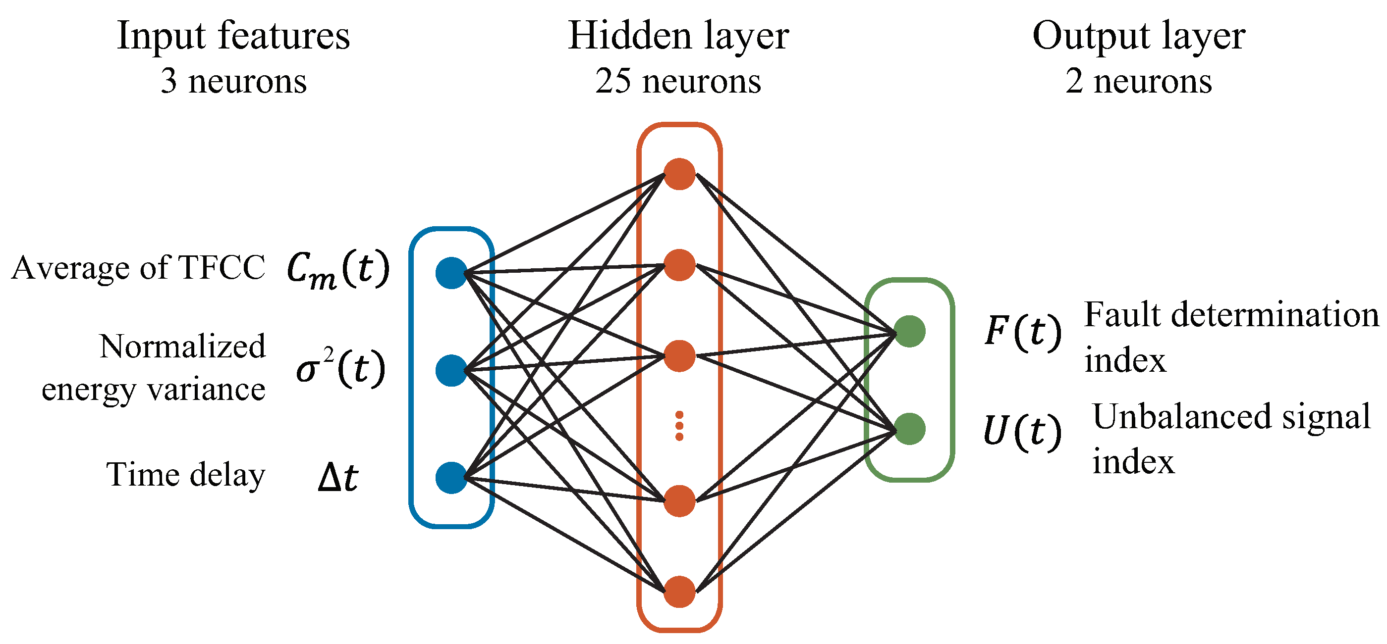
The ANN, a statistical learning algorithm inspired from neural networks in a biological nervous system is widely utilized in machine learning and cognitive sciences. Specifically, the ANNs are applied in function approximation, recognition, classification and pattern recognition. We used a multi-layer perceptron (MLP) which is a class of the feed-forward ANN to detect the fault location and to distinguish the cable connection points in a multi-core cable. The topological structure of the MLP used in this study is illustrated in Figure 2. The MLP consists of one input layer with three neurons, one hidden layer with 25 neurons, and one output layer with two neurons [23]. Since the number of hidden layers determines the performance of the data fitting process, an appropriate number of hidden layers is requisite.

In this study, the optimal hidden layer of the MLP is determined by the split-sample method. For the split-sample method, 50% of the data samples have been used for training and the remaining half has been used for testing. The activation function for the hidden layer was the hyperbolic tangent sigmoid function as follows:

$$f\left(x\right)=tanh\left(x\right)=\frac{2}{1+e^{-2x}}-1$$

(3)

where x and $f\left(x\right)$ are the input and output of the hidden neuron, respectively.

First, we set the thresholds of the average TFCC (${\mu }_1$) and the normalized variance (${\mu }_2$), respectively and classified the TFDR reflected signal cases in a multi-core cable as follows: (1) a normal cable junction, (2) a balanced fault, or faults in all lines, and (3) the unbalanced fault, or a partial line fault resulting in reflected signals due to both the fault and cross-talk. The threshold value of each input parameter was set with preliminary test results considering noise, signal interference, and cross-terms.

Next, the input features of the TFDR results for the MLP were set as time domains: average of the TFCC, the normalized energy variance of the reflected signals, and the time delay between the reference signal and the reflected signal. The time delay and the average of the TFCC are strongly relevant with the fault existence and location of the reflected data, respectively. In addition, the normalized energy variance of the reflected signals contain information on the presence of an incipient partial line fault. Partial line faults require the detection of faulty lines through classification before all lines become defective leading to devastating errors in the multi-core cable. The input features can be expressed as follows:

$$\begin{array}{cc}\hfill C_m\left(t\right)& =\frac{1}{N(N-1)}{\sum }_{i=1}^N{\sum }_{j=1}^N{C}_{ij}\left(t\right)\mathrm{for}i\ne j\end{array}$$

(4)

$$\begin{array}{cc}\hfill {\sigma }^2\left(t\right)& =E\left[{(r_{ij}\left(t\right)-r_m\left(t\right))}^2\right],\mathrm{for}i\ne j\end{array}$$

(5)

$$\begin{array}{cc}\hfill \delta t& =t_{r_{ij}}-t_s\end{array}$$

(6)

where i and j refer to the connected generation and victim line number, respectively. $r_{ij}\left(t\right)$ is the reflected signal with i-th generation/j-th victim line. $t_{r_{ij}}$ is the center time of $r_{ij}\left(t\right)$ and $t_s$ is the center time of the reference signal $s\left(t\right)$ which are expressed as follows:

$$\begin{array}{cc}\hfill t_{r_{ij}}& =\int t|r_{ij}{\left(t\right)|}^{2}dt\end{array}$$

(7)

$$\begin{array}{cc}\hfill t_s& ={\int t|s\left(t\right)|}^{2}dt.\end{array}$$

(8)

The output parameters were the fault determination index ($F\left(t\right)$) and the unbalanced signal index ($U\left(t\right)$). The fault determination index estimates the fault location, and the unbalanced signal index estimates the type of the fault. The dataset to train the MLP according to the averages of TFCC, normalized energy variance, and time delay were obtained by the simulated measured data considering the thresholds for each cable sample. The dataset was randomly divided into two separate sets, each for training (85%) and testing (15%). We employed a scaled conjugate gradient (SGC) back-propagation algorithm with a cross-entropy performance function [24]. Furthermore, the training process was ceased under the following conditions: (1) the maximum number of iterations (1000) is reached; (2) the maximum amount of time is exceeded; (3) the performance is minimized to the goal; or (4) the performance gradient falls below the target.

2.3. Line Classification Using Clustering Analysis

Following the detection and classification of the impedance discontinuity points, the clustering algorithm was used for differentiating faulty lines in the multi-core cable. The input features for clustering were the TFCC results and the phase synchrony index of each reflected data, which estimates the phase difference between the incident signal and the reflected signal to distinguish the characteristics of the fault. The phase synchrony between the incident and the reflected signal was estimated using the reduced interference Rihaczek time-frequency distribution, which provides a better localization for the phase-modulated signals and time-varying phases [25]. The phase difference between the incident signal and the reflected signal is computed as follows:

$${\varphi }_{sr}(t,\omega )=arg\left[\frac{R_s(t,\omega )}{|R_s(t,\omega )|}\frac{R_r^{*}(t,\omega )}{|R_r(t,\omega )|}\right].$$

(9)

The TFCC and the phase synchrony of the real impedance discontinuity point differ with the crosstalk signals. While, the TFCC values are related with the degree of the impedance discontinuity, phase difference is relevant to the type of impedance discontinuity. When at least one generation-victim line pair is defective, a reflected signal with a faulty line pair at the real impedance discontinuity point shows a high TFCC value. Estimated phase values are either the same (open) or the opposite (short) with those of the cable endpoints. Conversely, reflected signals caused by crosstalk have relatively lower TFCC values and show a different phase from actual defective lines. Therefore, a clustering analysis using the energy and phase properties of the reflected signal can be utilized to differentiate the faulty line.

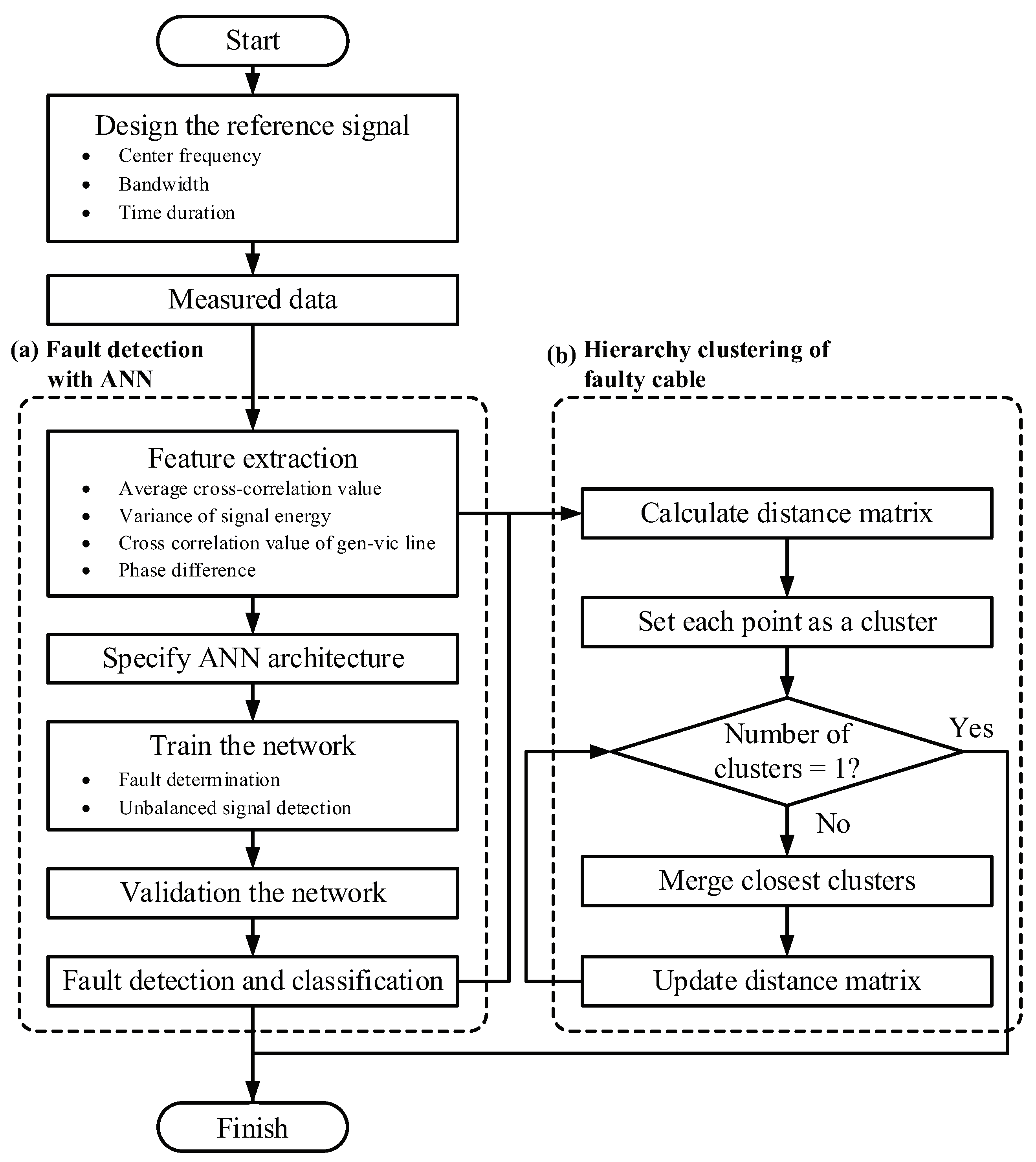
We used the hierarchy agglomerative clustering algorithm which allows each data to fit into multiple clusters with varying degrees of similarities. Hierarchy clustering is used for maximizing both the similarity within the cluster and the dissimilarities among clusters. First, the starting point for each data is in its own cluster, and the cluster pair merges as it rises above the hierarchy which continues until only a final cluster remains. Let $X=\left\{x_1,x_2,...,x_N\right\}$ be the data set. The hierarchy clustering process was done as follows:

(1)

Create the similarity matrix $D=\left[d_{ij}\right]$, where $d_{ij}$ is the distance between data samples using the following formula:

$$d_{ij}={\left(\sum _K{(x_i-x_j)}^2\right)}^{1/2}$$

(10)

where K is dimension of the data;

(2)

Find the closest pair of clusters and merge them into a single cluster;

(3)

Compute similarities between the new cluster and each of the old clusters;

(4)

Repeat steps (2) and (3) until all data are clustered into a single cluster of size N.

In the clustering process, the similarities among clusters are defined as the shortest distance between two points in each cluster which is expressed as follows:

$$L(X,Y)=\underset{x\in X,y\in Y}{min}d(x,y),$$

(11)

where X and Y indicate separate clusters.

In addition, the silhouette index was calculated for each data cluster in order to validate its accuracy and internal consistency. The silhouette of a cluster measures the similarity of its own data and compares it with other clusters. The silhouette index for data l, $s\left(l\right)$ can be expressed as follows: [26]

$$s\left(i\right)=\frac{b\left(l\right)-a\left(l\right)}{\max \left(a\left(l\right),b\left(l\right)\right)}$$

(12)

where $a\left(l\right)$ is the average dissimilarity of l with all the other data within the same cluster, $b\left(l\right)$ is the lowest average dissimilarity of data l with the data in the other clusters, (of which data l is not a member). $a\left(l\right)$ indicates how well data l is assigned to its cluster and $b\left(l\right)$ indicates how similar data l is to the data in neighboring clusters. The silhouette index ranges from −1 to 1; a higher silhouette value indicates clustering results of higher quality. An average silhouette index greater than 0.5 indicates reasonable partitioning of the data [27]. Figure 3 shows the overall fault detection and classification process for a multi-core cable, including the fault detection and faulty line classification steps.

3. Experimental Setup

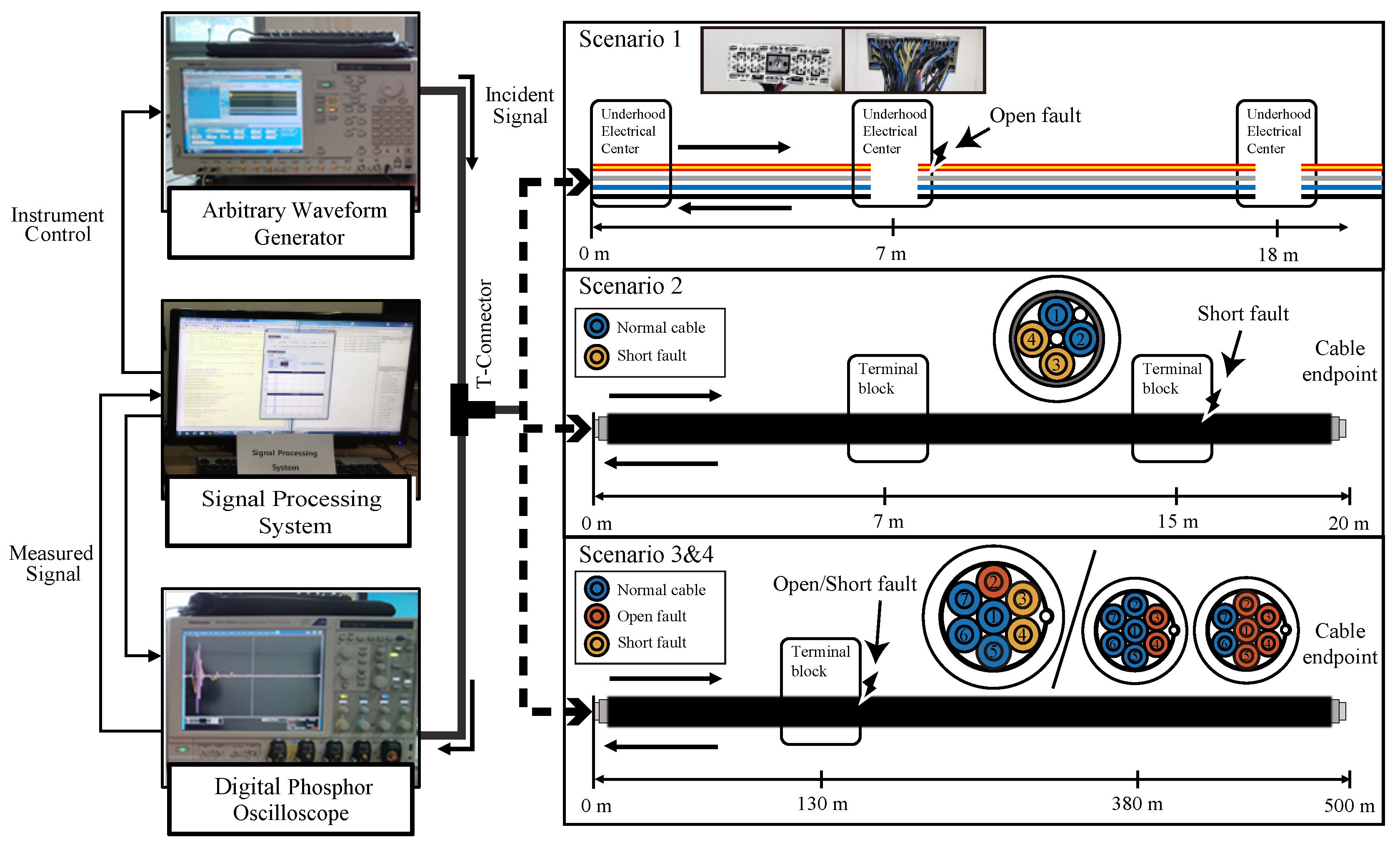
Figure 4 shows a schematic diagram of the proposed TFDR system. It consists of an incident signal generation part, a signal measurement part, and a signal processing part. After designing the optimal reference signal, the arbitrary waveform generator (AWG) creates the designed incident signal, and this signal is applied to the cable. Then, the digital storage oscilloscope (DSO) measures the reflected signal from the cable. Finally, the signal processing system receives the measured signal and performs a time-frequency analysis on it.

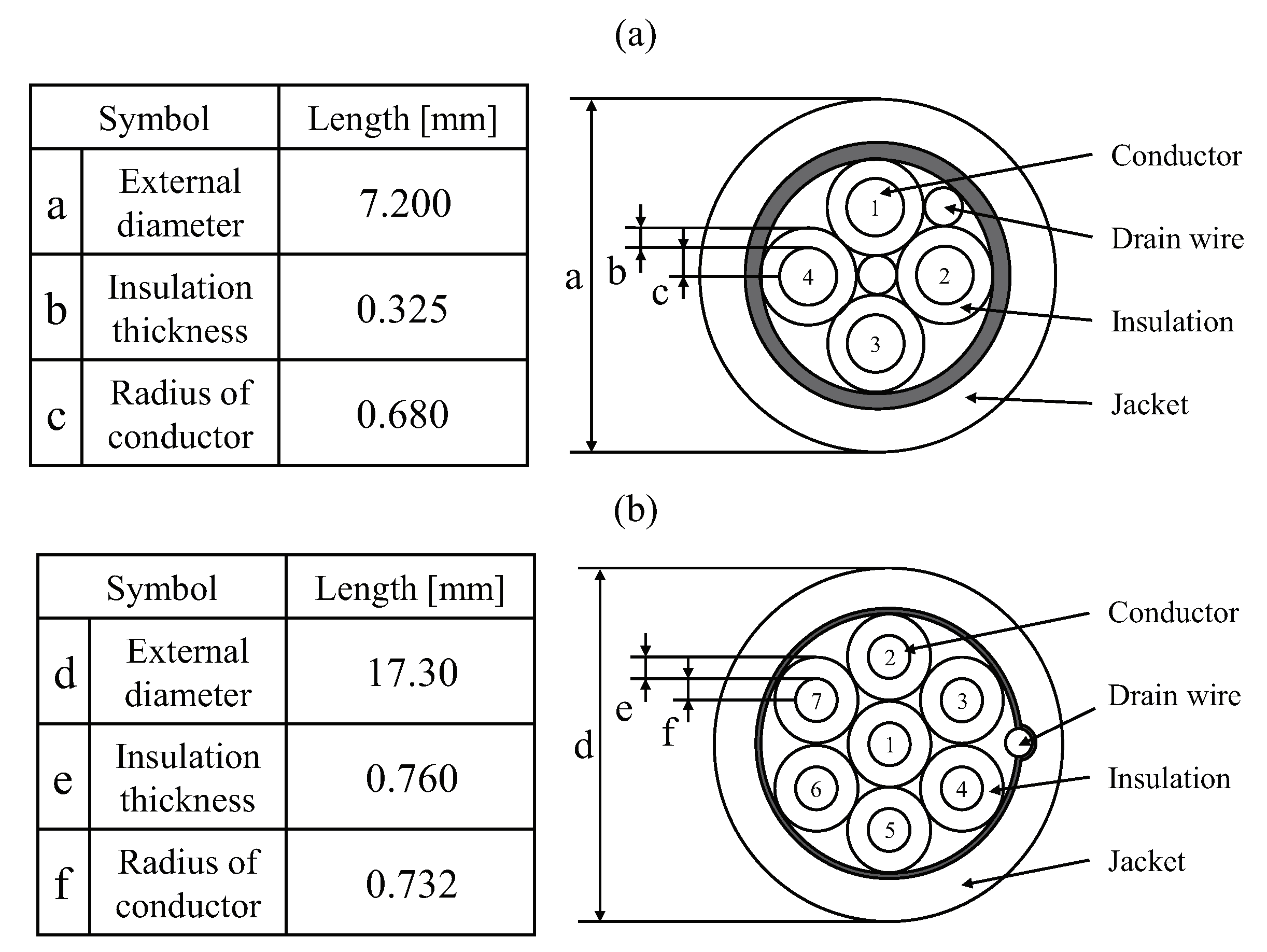
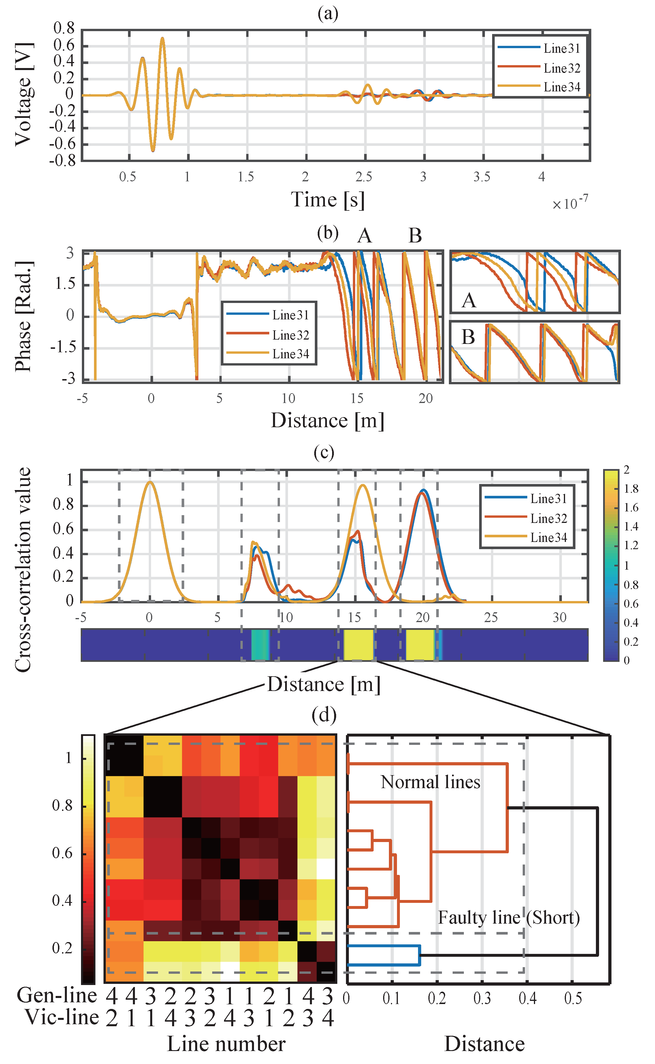
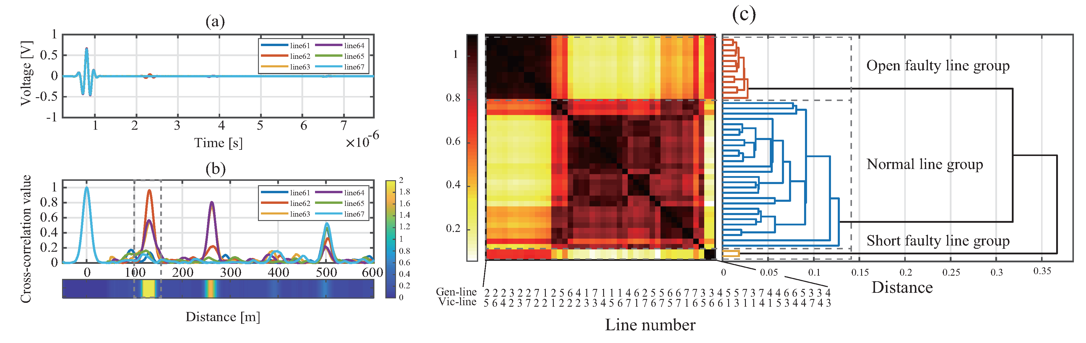
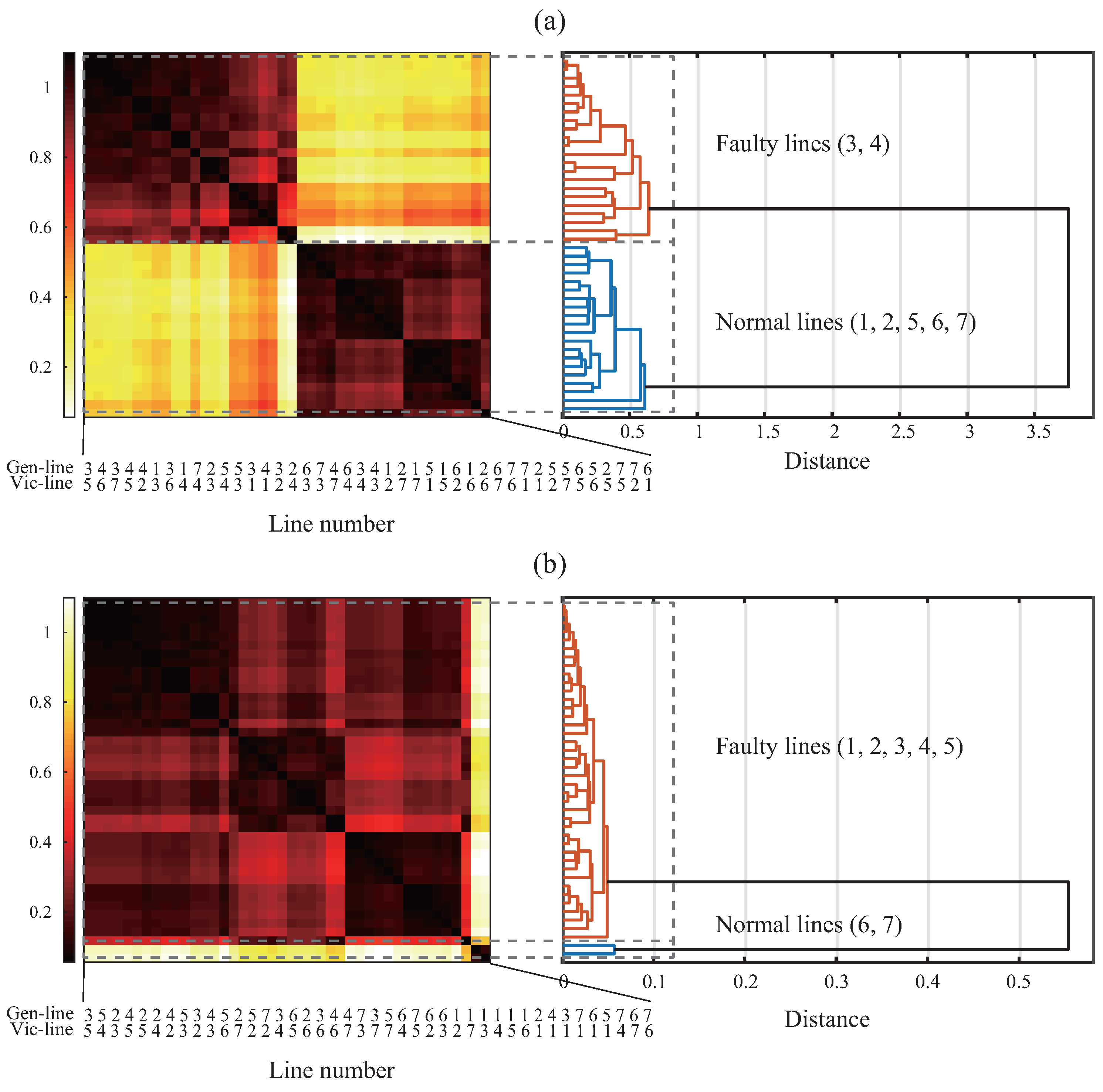
To verify the performance of the proposed algorithm for multi-core cable fault diagnosis, we simulated four fault scenarios using multi-core cables of varying types and lengths. The cable sample used for the first scenario consisted of four different wires of an automotive multi-wire with UEC connectors. Automotive wires possess the characteristics of lacking a jacket and having a single insulation layer for each core. The total length of the cable was 18 m, and the cable end was connected to another UEC connector. In the scenario, we emulated an open fault in the red line at 7 m of the UEC connector. We conducted the fault location detection and the differentiation of the actual faulty line among automotive wires. In the second scenario, a short fault at one of two terminal blocks (15 m) was emulated in a four-core 20 m length C&I cable of an NPP. In other words, both a normal and faulty cable junction coexist in the same cable. In the third scenario, a combination of an open and short fault was emulated in a seven-core C&I cable. In specific, one line was opened, and two lines were shorted at the terminal block (130 m). In the final scenario, an open fault due to physical stress from one external direction was emulated in the same seven-core C&I cable used in a previous scenario. Here, we detected the faulty lines of the cable and additionally estimated the direction of the external physical stress at the terminal block. The total lengths of the C&I cable samples for scenarios 3 and 4 were both 500 m with a Class 1E. The cable cross sections of the experiments are illustrated in Figure 5. The algorithm was initially applied in long cables when using multi-core C&I cables. However, acknowledging that wires in automotive vehicles are generally installed in limited spaces, the proposed algorithm was targeted at short-length cables for experiments using automotive wires.

4. Results and Discussion

4.1. An Open Fault in an Automotive Line

Among four lines with different colors (red, grey, black blue), the red line was opened at the UEC connector while others intact. In these lines, 12 reflected signals were measured.

Figure 6 shows the fault detection and classification results with the blue line as the generation line. Figure 6a,b represent the reflected signals in the time domain and the phase estimation results, respectively. Since the reflected signals are much smaller than that of the incident signal, time-domain results are incapable of determining neither the fault location nor the faulty line. The phase at the UEC connector with a faulty line pair is zero whereas that of normal line pairs are not. The TFCC results amplify the value at the impedance discontinuity point, as illustrated in Figure 6c. TFCC results show that the UEC connector is commonly detectable in every line pair data with differing degrees depending on the victim line. Since line blue-red showed the highest value of all possible line pairs as shown in Figure 6c, the TFCC results can be utilized in deciphering fault occurrence and location. The line classification results of the reflected signals obtained via the ANN are shown as an image under the plot of Figure 6c. The line classification results are expressed as the sum of $F\left(t\right)$ and $U\left(t\right)$ to intuitively interpret the results. The maximum value indicates a partial fault occurring at the cable junction. In addition, a value of 1 indicates that the entire cable is defective due to external stress or the case of a reflected signal measured at the cable junction point in a normal cable. The results show that the faulty UEC connector is detected at 7 m except the input mismatch at 4 m.

The heat-map was used to identify the clustering results between each signal data. The heat-map shows the normalized Euclidean distance of each 2D data (TFCC results and phase synchrony index) according to its similarity. Therefore, as the distance increases the irrelevance between the data grows as well. In addition, the actual fault wire can be distinguished from the normal wire in the multi-core cable. The number of clusters was set to the number of sudden jumps in the dendrogram which was set to 0.5241 of maximum distance. The clustering results showed that the reflected signal at the UEC connector can be classified into two groups which is illustrated in Figure 6d. The clustering results revealed that the entire data set from the first group included the red line in the generation line or the victim line.

Therefore, when an open fault occurs in a multi-core cable, all pairs of the connected lines are clustered into the same group. The first group possessed a high TFCC value and centered around the phase value of zero. On the other hand, the feature data in the second group showed lower TFCC values but had higher phase values. The centroid and the variance of each cluster are summarized in

Table 1. Fault location and clustering results.

Fault Scenarios		Cluster	Fault Location			Centroid		Average Silhouette Score
			Actual Location (m)	Detection Results (m)	Error (%)	TFCC	Estimated Phase (rad.)
Automotive lines (Open fault)		Faulty lines	9	8.525	5.28	0.842	−0.580	0.984
		Normal lines		9.561	6.23	0.538	2.627	0.938
Four-core C&I cable (Short fault)		Faulty lines	8	7.818	2.28	0.973	−2.831	0.999
		Normal lines		7.901	1.24	0.357	−1.886	1.000
Seven-core C&I cable (Open/Short fault)		Open fault lines	130	129.1	0.69	0.900	−0.532	0.856
		Short fault lines		129.8	0.15	0.973	3.186	0.998
		Normal lines	132.6	2.00	0.173	−0.975	0.875
Seven-core C&I cable (Open fault)	First floor (Lines 3 and 4)	Faulty lines	380	381.2	0.32	0.635	0.040	0.968
		Normal lines		$·$	$·$	0.033	−1.358	0.937
	First and second floor Lines 1, 2, 3, 4 and 5)	Faulty lines	380	380.5	0.13	0.761	−0.128	0.957
		Normal lines		$·$	$·$	0.028	1.639	0.995

. All silhouette indexes for the clustering results are more than 0.9 which indicate that the line pair data was well clustered using the time-frequency features. The total line pair data classified as a faulty line contained a red line as the generation line or the victim line. Combining the fault location and clustering results at the UEC connector allows the detection of the fault location and the segregation of the reflected signals from faulty line pairs (Lines red-blue, red-black, red-grey, blue-red, black-red, and grey-red) from those of normal line pairs (Lines blue-black, blue-grey, black-blue, black-grey, grey-blue, grey-black).

4.2. A Short Fault of a Faulty Line at the Terminal Block

The ANN with TFDR results were applied to detect a short fault at the terminal block. Short faults were applied to one of the two terminal blocks (15 m) at ines red-blue, red-black, red-grey, blue-red, black-red, and grey-red) from those of normal line pairs (Lines blue-black, blue-grey, black-blue, black-grey, grey-blue, grey-black). 3 and 4. Figure 7 shows the fault detection and classification results with Line 3 as the generation line. We refer to the reflected signal of each line pair using the number of the generation line followed by the number of the victim line. For instance, Line 3-4 points to the TFDR results with Line 3 as the generator line and Line 4 as the victim line. TFCC and ANN results indicate that the terminal block at 8 m was balanced and thus not defective, whereas the faulty terminal block at 15 m was unbalanced with the cable endpoint due to dissimilarities between the faulty line pair and the normal line pair data, as illustrated in Figure 7c. The clustering results at the unbalanced terminal block are illustrated in Figure 7d. By clustering at the terminal block, the multi-core diagnostic data was classified into two clusters. One corresponds to line pairs where a short fault occurred (Lines 3-4, 4-3), and the other contains the rest. Normal lines can be discerned from short faulty line pairs through the energy differences of the reflected signals. In addition, clustering results reveal that the pair data of only short fault lines can be distinguished from the pair data of other lines which possess features different from an open fault case.

4.3. A Combination of Open and Short Faults at the Terminal Block

In a seven-core C&I cable, short faults were emulated in Lines 3 and 4, and the open fault was applied to Line 2 at the terminal block. Figure 8 shows the fault detection and classification results with Line 6 as the generation line. The results of the TFCC and ANN indicate that the terminal block at 130 m was determined as an unbalanced fault point through the differences between the faulty line pair and the normal line pair data, as illustrated in Figure 8b. Therefore, the reflected signals at the faulty terminal block (130 m) require clustering to determine the faulty line. Next, hierarchy clustering was applied to the reflected signals at the unbalanced fault point. The multi-core diagnostic data was classified into three clusters which is shown in Figure 8c. One corresponds to line pairs where the short fault occurred(Lines 3-4, 4-3). Another contains all line pairs including Line 2, where an open fault occurred, and the last one contains the rest. In the open fault case, all lines including the open fault line (Line 2) were clustered. On the other hand, only the faulty line pair data (Line 3-4) was clustered in the short fault. The phase of the normal line pairs is normally close to zero but was slightly below zero due to short fault crosstalk. Normal line pair data have low TFCC values, but the phases are long distributed due to the crosstalk. The centroid and the variance of each cluster are summarized in Table 1. The results show that it is possible to detect an open fault in all related faulty line pair data whereas the short fault is detected only in a line where a short fault occurs. Thus, open and short faulty lines in multi-core cables can be detected even with combined faults occurring at the same point.

4.4. Multi-Core Cable Diagnosis according to the Number of Faulty Lines

We analyzed the clustering results for reflected signals of an opened multi-core cable induced by a one-way physical stress from the cable exterior. Seven lines in the cable are divided into 3 floors and the open fault was emulated in each floor.

Figure 9a shows the clustering results for when Lines 3 and 4 (first floor) are opened. The results show that the line pair data of the faulty line was successfully distinguished from the normal line pair data despite shared features of the open fault case in Figure 6d. Normal line pair data possess low TFCC values and long distributed values in phase axis due to crosstalk. Next, Figure 9b illustrates the clustering results for when open faults occurred in the second floor (Lines 1, 2, 3, 4, and 5). The reflected signal data of the normal line from previous results (Lines 1, 2, and 5) shifted to the faulty line pair group. The centroid and the variance of each cluster are summarized in Table 1. When the number of open fault lines increased, TFCC values increased likewise due to the increase in faulty reflected signals, while the phase remained unaltered. In addition, the TFCC of normal line pair data was low and the fault could not be detected even when the fault occurred in a multi-core cable. Therefore, all line pairs in the multi-core cable should be considered for all possible fault detection and classification. All average silhouette scores exceeded 0.93 indicating that the fault line data was well classified. Consequently, fault clustering using the proposed method allows the classification of cable structure and the detection of the faulty line. In addition, monitoring changes in the clustering results allow the determination of changes in condition of each line.

5. Conclusions

In this paper, we proposed a fault detection and classification method in a multi-core cable using the ANN and hierarchy clustering based on TFDR results. The fault and cable junction can be detected and differentiated considering the location of the fault and the unbalance level of the reflected signals. Our classification and clustering results which were verified in four fault scenarios in multi-core cables (automotive lines and C&I multi-core cables), achieved the differentiation between faulty and normal line pairs along with the identification of the fault in a multi-core cable regardless of cable length.

This method can be used for monitoring the overall condition of a multi-core cable through quantitatively tracking for changes in clustering results which enables condition-based maintenance. In short, this method can be applied for the health index of cables by analyzing the degradation tendency in a multi-core cable using feature changes of the TFDR results.